Theses Thesis/Dissertation Collections
1-20-2012
Techniques for automatic large scale change
analysis of temporal multispectral imagery
Ryan MercovichFollow this and additional works at:http://scholarworks.rit.edu/theses
This Dissertation is brought to you for free and open access by the Thesis/Dissertation Collections at RIT Scholar Works. It has been accepted for inclusion in Theses by an authorized administrator of RIT Scholar Works. For more information, please [email protected].
Recommended Citation
Techniques for Automatic Large Scale
Change Analysis of Temporal
Multispectral Imagery
By
Ryan A. Mercovich
A dissertation submitted in partial fulfillment of the requirements for the degree of Doctor of Philosophy in the Chester F. Carlson Center for Imaging Science at the Rochester Institute of Technology
1/20/2012
Signature of the Author Date
CHESTER F. CARLSON CENTER FOR IMAGING SCIENCE ROCHESTER INSTITUTE OF TECHNOLOGY
ROCHESTER, NEW YORK
CERTIFICATE OF APPROVAL
Ph.D. DEGREE DISSERTATION
The Ph.D. Degree Dissertation of Ryan A. Mercovich has been examined and approved by the dissertation committee as satisfactory for the dissertation required for the Ph.D. degree in Imaging Science
Dissertation Advisor:
Dr. David W. Messinger
Committee Member:
Dr. Anthony Vodacek
Committee Member:
Dr. William F. Basener
External Chair:
CHESTER F. CARLSON CENTER FOR IMAGING SCIENCE ROCHESTER INSTITUTE OF TECHNOLOGY
ROCHESTER, NEW YORK
DISSERTATION RELEASE PERMISSION
Ph.D. DEGREE DISSERTATION
I, Ryan A. Mercovich, hereby grant permission to the Wallace Memorial Library of R.I.T. to reproduce my dissertation in whole or in part. Any reproduction will not be for commercial use or profit.
i
Techniques for Automatic Large Scale Change Analysis of Temporal Multispectral Imagery
Ryan A. Mercovich
Chester F. Carlson Center for Imaging Science College of Science,
Rochester Institute of Technology
Abstract
Change detection in remotely sensed imagery is a multi-faceted problem with a wide variety of desired solutions. Automatic change detection and analysis to assist in the coverage of large areas at high resolution is a popular area of research in the remote sensing community. Beyond basic change detection, the analysis of change is essential to provide results that positively impact an image analyst’s job when examining potentially changed areas. Present change detection algorithms are geared toward low resolution imagery, and require analyst input to provide anything more than a simple pixel level map of the magnitude of change that has occurred. One major problem with this approach is that change occurs in such large volume at small spatial scales that a simple change map is no longer useful. This research strives to create an algorithm based on a set of metrics that performs a large area search for change in high resolution multispectral image sequences and utilizes a variety of methods to identify different types of change. Rather than simply mapping the magnitude of any change in the scene, the goal of this research is to create a useful display of the different types of change in the image.
The techniques presented in this dissertation are used to interpret large area images and provide useful information to an analyst about small regions that have undergone specific types of change while retaining image context to make further manual interpretation easier. This analyst cueing to reduce information overload in a large area search environment will have an impact in the areas of disaster recovery, search and rescue situations, and land use surveys among others. By utilizing a feature based approach founded on applying existing statistical methods and new and existing topological methods to high resolution temporal multispectral imagery, a novel change detection methodology is produced that can
iii Table of Contents
Abstract ... i
Table of Contents ... iii
List of Figures ... v
List of Tables ... ix
Chapter 1: Introduction ... 1
1.1 Project Description ... 2
1.2 Overview ... 3
1.3 Objectives ... 6
Chapter 2: Background ... 7
2.1 Identifying Image Changes ... 8
2.2 Data Assumptions ... 9
2.3 Existing Methods ... 10
2.4 Chapter summary... 25
Chapter 3: Topological Clustering ... 27
3.1 Modularity clustering ... 28
3.2 Verification with simple data ... 34
3.3 Edge identification and graph creation ... 37
3.4 Chapter summary... 43
Chapter 4: Change Analysis ... 45
4.1 Feature based algorithm ... 46
4.2 Cross image equalization ... 47
4.3 Spatial image segmentation ... 58
4.4 Classifying change ... 61
4.5 Change metrics ... 69
4.6 Visualization of change detections ... 96
4.7 Chapter summary... 97
Chapter 5: Experimental Verification ... 99
5.1 Data ... 99
iv
5.3 Experiment B: Assessing edge identification ... 115
5.4 Experiment C: Initial analysis of modularity ... 120
5.5 Experiment D: Further modularity testing ... 131
5.6 Experiment E: Enumerating clusters in a data cloud ... 144
5.7 Experiment F: Assessment of tile based change metrics ... 147
Chapter 6: Change Analysis Results ... 177
6.1 Initial Results ... 177
6.2 Full image analysis ... 179
Chapter 7: Summary ... 207
7.1 Change detection framework ... 208
7.2 Important change detection concepts ... 212
7.3 Idealized versus realistic change analysis ... 213
7.4 Outcomes and Applications ... 214
7.5 Future work ... 215
References ... 225
Appendices ... 233
7.6 Appendix A ... 233
7.7 Appendix B: Display scaling of matched images in ENVI ... 233
7.8 Appendix C: Supplemental plots ... 238
v
List of Figures
FIGURE 1:WORLD VIEW 2 RELATIVE SPECTRAL RESPONSE ... 4
FIGURE 2:WV2 SATELLITE SENSING PLATFORM CHARACTERISTICS ... 4
FIGURE 3:SPECTRAL AND SPATIAL RESOLUTION OF SEVERAL SENSING SYSTEMS. ... 5
FIGURE 4:EXAMPLE SCENE TO SCENE CHANGES ... 8
FIGURE 5:CHANGE VECTOR ANALYSIS EXAMPLE. ... 11
FIGURE 6:EXAMPLE POST CLASSIFICATION CHANGE DETECTION ... 16
FIGURE 7:PDP PLOTS FOR A SIX CLASS IMAGE . ... 18
FIGURE 8:EXAMPLE 𝚫𝑷𝑫𝑻𝑳 PLOT USED TO DETECT CHANGE. ... 18
FIGURE 9:AN AREA WHERE K-MEANS IS STILL USEFUL AND ONE WHERE IT CAUSES CONFUSION ... 22
FIGURE 10:GRADIENT FLOW, REPRODUCED FROM BASENER. ... 24
FIGURE 11:EXAMPLE OF EDGE CREATION AND CLUSTERING. ... 29
FIGURE 12:AN EXAMPLE OUTPUT OF GROUP SPLITTING WITH MODULARITY. ... 32
FIGURE 13:EXAMPLE MODULARITY VARIABLE LEVEL OF DETAIL CLUSTER MAP ... 33
FIGURE 14:THE DATA AND ITS GRAPH. ... 34
FIGURE 15:K-MEANS CLUSTERINGS. ... 36
FIGURE 16:MODULARITY CLUSTERING, CONVERGENCE AFTER 5 LEVELS. ... 36
FIGURE 17:AN EXAMPLE CONSTRUCTION FOR A GRID GRAPH. ... 38
FIGURE 18:THE LOCALLY WEIGHTED METHOD TAKES SPECTRALLY SIMILAR PIXELS FROM… ... 40
FIGURE 19:CO-DENSITY DISTRIBUTION FOR 80 NEIGHBORS OF AN IMAGE. ... 42
FIGURE 20:EXAMPLE CHANGE TYPES AND CHANGE ANALYSIS WORKFLOW. ... 47
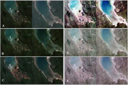
FIGURE 21:EXAMPLE RESULT OF HISTOGRAM MATCHING TECHNIQUES... 48
FIGURE 22:ORIGINAL GEOEYE HAITI IMAGERY DISPLAYED USING RAW IMAGE COUNTS ... 50
FIGURE 23:MANY EQUALIZATION METHODS FOR THE HAITI IMAGE SET. ... 51
FIGURE 24:DATA CLOUDS BEFORE AND AFTER COVARIANCE EQUALIZATION. ... 52
FIGURE 25EXAMPLE CROSS IMAGE CALIBRATION BY LINEAR SHIFT. ... 54
FIGURE 26:FLIE EQUALIZATION OF HAITI 2010 IMAGE SET. ... 55
FIGURE 27:SPATIAL IMAGE SEGMENTATION—EXAMPLE OVERLAPPING SCHEME ... 59
FIGURE 28:TILE SIZE EXAMPLE, BASE IMAGE LEFT, CHANGE IMAGE RIGHT. ... 60
FIGURE 29:SEVERAL SUPERPIXEL SEGMENTATIONS OF AN RGB IMAGE. ... 61
FIGURE 30:EACH TYPE OF CHANGE COULD BE CLASSIFIED BY THE COMBINATION OF … ... 61
FIGURE 31:EXAMPLE SMALL SCALE CHANGE.SOCCER GOALS PLACED IN A FIELD. ... 64
FIGURE 32:EXAMPLE OF LARGE SCALE CHANGE.A NEW PARKING LOT. ... 64
FIGURE 33:EXAMPLE SMALL SCALE CHANGE IN THE DATA SPACE. ... 67
FIGURE 34:EXAMPLE OF LARGE SCALE CHANGE IN THE ND SPACE. ... 67
FIGURE 35:THE SPECTRAL ANGLE SPECTRAL SIMILARITY METRIC MEASURES … ... 73
FIGURE 36:AN EXAMPLE TREE SHOWING THE GROUP IDENTITY … ... 75
FIGURE 37:TILES FROM TIME 1 AND TIME 2 WITH WIDESPREAD SUBTLE CHANGE … ... 77
FIGURE 38:EXAMPLE IMAGES WITH EDGE LENGTH HISTOGRAM PLOTS. ... 80
FIGURE 39:EXAMPLE DISTRIBUTIONS WITH CHANGING OUTLIER CLUSTERS. ... 81
FIGURE 40:𝑵𝑬𝑽 PLOTS FOR FOUR COMPARISONS OF FOUR SETS OF DATA. ... 83
FIGURE 41:NEV PLOTS VERSUS NUMBER OF NEIGHBORS USING A SUBSET OF … ... 85
FIGURE 42:EXAMPLE 2D DATA AND HISTOGRAMS OF TOTAL CO-DENSITY ... 87
FIGURE 43:EXAMPLE DATA FROM TWO DATA SETS WITH THEIR ASSOCIATED 𝑨𝑵𝑫 PLOTS ... 89
FIGURE 44:𝑨𝑵𝑫 PLOTS FOR A SINGLE GAUSSIAN DISTRIBUTION. ... 90
FIGURE 45:𝑨𝑵𝑫 PLOTS FOR A UNIFORM DISTRIBUTION ... 91
FIGURE 46:𝑨𝑵𝑫 PLOTS FOR TWO EQUAL COVARIANCE GAUSSIAN DATASETS. ... 92
vi
FIGURE 48:EXAMPLE OUTPUT FROM CHANGE DETECTION. ... 97
FIGURE 49:FLOW CHART FOR FEATURE BASED CHANGE ANALYSIS. ... 98
FIGURE 50:CROPPED RGBHYMAP IMAGE FROM COOKE CITY,MT ... 100
FIGURE 51:PART OF RIT’S CAMPUS CAPTURED WITH MISIJUNE 21 AND 24. ... 101
FIGURE 52:COMPASS HYPERSPECTRAL IMAGE WITHOUT AND WITH CHANGE TARGETS. ... 101
FIGURE 53:HYDICE FOREST SCENE WITH AND WITHOUT EXPOSED TARGETS. ... 102
FIGURE 54:EXAMPLE SECTION OF BEFORE AND AFTER QUICKBIRD TSUNAMI IMAGERY. ... 103
FIGURE 55:CROPPED GEOEYE-1 IMAGE OVER HAITI, PRE- AND POST-EVENT ... 103
FIGURE 56:WORLD VIEW 2 IMAGERY OF ROCHESTER IN JUNE AND SEPTEMBER OF 2010 ... 104
FIGURE 57:NDVI IMAGES AND LUMINOSITY HISTOGRAMS FOR THE ROCHESTER SCENE …. ... 105
FIGURE 58:THE RELATIVE SPECTRAL RESPONSE FOR WORLDVIEW-2. ... 106
FIGURE 59:ILLUSTRATION OF EXTREME REGISTRATION ERROR DUE TO THE CAMERA VIEW... 107
FIGURE 60:WV2 SENSOR ARRAY DIAGRAM. ... 108
FIGURE 61:WV2 BANDS FROM DIFFERENT MULTISPECTRAL GROUPS SHOW MISREGISTRATION ... 109
FIGURE 62:CROP OF THE 2006 AERIAL HYPERSPECTRAL IMAGE OVER RIT. ... 114
FIGURE 63:CHANGE MAPS FROM HYPERSPECTRAL AND WV2 RESAMPLING. ... 114
FIGURE 64:SECOND RIT2006 CROPPED REGION WITH CHANGE MAPS. ... 115
FIGURE 65:THE DATA USED FOR ANALYSIS COMES FROM THE HYDICE FOREST RADIANCE SCENE. ... 116
FIGURE 66:THE GRAPH AND FIRST MODULARITY SPLIT WITH CLUSTER MAP OVERLAY ... 117
FIGURE 67:THIS PLOT OF THE GRAPH USING THE DENSITY WEIGHTED KNN ... 118
FIGURE 68:THREE 2-CLASS CLUSTER MAPS FOR MODULARITY AND N-CUTS ... 119
FIGURE 69:ERROR IMAGES ARE SHOWN FOR THE SIMPLE AND DENSITY WEIGHTED METHODS. ... 119
FIGURE 70:RESULTS OF MODULARITY CLUSTERING. ... 120
FIGURE 71:IMAGERY USED FOR MODULARITY CLUSTERING ... 121
FIGURE 72:IMAGE DATA CLOUDS FOR FOR THE COMPOSITE IMAGES. ... 123
FIGURE 73:THE SECOND TEST IMAGE AND ITS GML BASED MANUAL CLASSIFICATION MAP ... 124
FIGURE 74:THE MODULARITY CLUSTERING PROCESS FOR THE 6 CLASS TEST IMAGE ... 125
FIGURE 75:THE MODULARITY CLUSTERING PROCESS IN PROGRESS ... 126
FIGURE 76:IMAGE ONE THE RESULTS FOR K-MEANS,ISODATA, GRADIENT FLOW, AND MODULARITY ... 127
FIGURE 77:THE CLUSTER MAPS FOR THE REPRESENTATIVE TILE ... 130
FIGURE 78:ONE OF THE 1000 SIX CLASS AND EIGHT CLASS IMAGES ... 133
FIGURE 79:ALL THE PIXELS FOR THE EIGHT CLASSES (2500-6000 PER CLASS). ... 134
FIGURE 80:A DIFFERENT PROJECTION OF THE WATER PIXELS FROM FIGURE 79 ... 135
FIGURE 81:THE GRASS PIXELS DISPLAYED IN A NEW PROJECTION. ... 136
FIGURE 82:MODULARITY RESULTS FOR 1000 SIX CLASS TRIALS. ... 139
FIGURE 83:K-MEANS ACCURACY AND CLUSTERS PER TILE RESULTS FOR 1000 SIX CLASS TRIALS. ... 140
FIGURE 84:MODULARITY ACCURACY AND CLUSTERS PER TILE RESULTS. ... 141
FIGURE 85:K-MEANS ACCURACY AND CLUSTERS PER TILE RESULTS. ... 142
FIGURE 86:THREE RANDOMLY CHOSEN RUNS FROM THE EIGHT CLASS IMAGE. ... 143
FIGURE 87:REAL IMAGE TILES, ONE FROM HYDICE AND TWO FROM WV2. ... 144
FIGURE 88:EXAMPLE PEAK DETECTION FOR 6 CLASS CASE, WATER PEAKS HIGHLIGHTED. ... 146
FIGURE 89:EXAMPLE OF NOISE CAUSING IDENTIFICATION OF FALSE PEAKS. ... 146
FIGURE 90:EXAMPLE OF PIF CORRECTED IMAGE FOR SEPTEMBER AND JUNE. ... 149
FIGURE 91:SPECTRAL PROFILE COMPARISON FOR PIF NORMALIZATION. ... 150
FIGURE 92:ATMOSPHERIC TRANSMITTANCE SHOWING THE WV2 WINDOW. ... 150
FIGURE 93:PSEUDO-SYNTHETIC TILES CREATED FOR FOUR IMAGE STATES. ... 153
FIGURE 94:TILE 1 AND ITS 3-BAND PROJECTED DATA CLOUD FOR EACH IMAGE STATE. ... 155
FIGURE 95:RELATIVE CHANGE SCORES FOR PSEUDO-SYNTHETIC TILE 1. ... 156
FIGURE 96:ALL METRIC SCORES, PSEUDO-SYNTHETIC TILE 1. ... 157
vii
FIGURE 98:TILE 2 AND ITS DATA CLOUD (3-BAND PROJECTION) FOR EACH IMAGE STATE. ... 158
FIGURE 99:PLOTS FOR THE RELATIVE AND SCALED SCORES FOR PSEUDO-SYNTHETIC TILE 2... 159
FIGURE 100:TILE 3 AND DATA CLOUD AT EACH IMAGE STATE. ... 160
FIGURE 101:RELATIVE SCORES, PSEUDO-SYNTHETIC TILE 3. ... 161
FIGURE 102:SELECTED CHANGE METRICS, TILE 3. ... 161
FIGURE 103:OUTLIER SENSITIVE METRICS FOR TILE 3. ... 162
FIGURE 104:TILE 4 AND DATA CLOUD FOR EACH IMAGE STATE. ... 163
FIGURE 105:SCORES FOR ALL METRICS, PSEUDO-SYNTHETIC TILE 4. ... 163
FIGURE 106:TWO CHANGE SCORE GROUPS FOR PSEUDO-SYNTHETIC TILE 4. ... 164
FIGURE 107:TILE 5 AND DATA CLOUD FOR EACH IMAGE STATE. ... 165
FIGURE 108:PSEUDO-SYNTHETIC TILE 5 CHANGE METRICS. ... 165
FIGURE 109:TILE 6 AND DATA CLOUD FOR EACH IMAGE STATE. ... 166
FIGURE 110:RELATIVE SCORES FOR AL METRICS, PSEUDO-SYNTHETIC TILE 6. ... 166
FIGURE 111:METRIC SCORES FOR EACH COMPARISON IMAGE PAIR, TILE 6. ... 167
FIGURE 112:TILE 7 AND DATA CLOUDS FOR EACH IMAGE STATE. ... 168
FIGURE 113:NORMALIZES METRIC SCORES FOR TILE 7. ... 169
FIGURE 114:TILE 8 WITH DATA CLOUDS FOR EACH STATE... 170
FIGURE 115:SCALED CHANGE METRIC SCORES FOR TILE 8. ... 171
FIGURE 116:TILE 9 AND DATA CLOUDS FOR EACH STATE. ... 172
FIGURE 117:METRIC SCORES FOR PSEUDO-SYNTHETIC TILE 9. ... 173
FIGURE 118:TILE 10 WITH DATA CLOUDS FOR EACH STATE. ... 174
FIGURE 119:TIME 1 BASE AND TIME 2 CHANGE PSEUDO-SYNTHETIC IMAGES. ... 175
FIGURE 120:FULL IMAGE RELATIVE CHANGE SCORE FOR TIME 1 BASE TO TIME 2 CHANGE. ... 175
FIGURE 121:TIME 1 BASE AND TIME 2 BASE PSEUDO-SYNTHETIC IMAGES. ... 176
FIGURE 122:FULL IMAGE RELATIVE SCORES FOR T1B/T2B. ... 176
FIGURE 123:EXAMPLE RESULT FROM CLUSTER TREE BASED CHANGE DETECTION ... 177
FIGURE 124:COMPARISON RESULT FROM HYPERBOLIC CHANGE DETECTION. ... 178
FIGURE 125:ORIGINAL INDONESIA,2004TSUNAMI IMAGES.. ... 182
FIGURE 126:FULL IMAGE RESULTS FOR INDONESIA 2004. ... 183
FIGURE 127:AN AREA OF HEAVY DESTRUCTION AND LARGE SCALE DRAMATIC CHANGE ... 184
FIGURE 128:AN AREA WITH VERY LITTLE DAMAGE AND LOW CHANGE ... 185
FIGURE 129:THE SAME REGION AS IN FIGURE 128 FOR PDTL AND CO-DENSITY ESTIMATE. ... 186
FIGURE 130:THE SINGLE HIGHLIGHTED TILE SHOWING A BOAT. ... 186
FIGURE 131:CO-DENSITY (TOP) AND 𝚫𝑷𝑫𝑻𝑳 TOP 10% CHANGE MAPS. ... 187
FIGURE 132:FALSE ALARM IN PDTL SCORE.DATA CLOUDS FOR BASE IMAGE ... 188
FIGURE 133:FALSE ALARM IN CO-DENSITY CLUSTER ESTIMATE SCORE. ... 189
FIGURE 134:ROCHESTER 2010 IMAGE SET, CALIBRATED AND EQUALIZED. ... 191
FIGURE 135:CHANGE MAP FOR COMBINED SCORES,ROCHESTER,2010.. ... 192
FIGURE 136:RIT CAMPUS PORTION OF THE ROCHESTER 2010 IMAGE SET. ... 193
FIGURE 137:COMBINED RESULT RIT DETAIL ... 194
FIGURE 138:CHANGE RESULTS FOR RIT CAMPUS DETAIL.. ... 195
FIGURE 139:COMPARISON OF SPECTRAL REFLECTION AND WHITE TENTS. ... 197
FIGURE 140:EXAMPLE MISSED DETECTION IN ROCHESTER 2010 DATASET. ... 198
FIGURE 141:DATA CLOUD FOR PARKING LOT WITH TENTS, AND CARS. ... 198
FIGURE 142:2010HAITI EARTHQUAKE PRE- AND POST-EVENT. ... 200
FIGURE 143:HAITI 2010 EARTHQUAKE IMAGE CHANGE MAP RESULTS. ... 201
FIGURE 144:IMPACT OF SPECTRAL SAMPLING ON CHANGE IDENTIFICATION. ... 202
FIGURE 145:NDVI CHANGE USED TO IDENTIFY INTERESTING CHANGES ... 204
FIGURE 146:MODULARITY CLUSTER NUMBER CHANGE USED DIRECTIONALLY ... 205
viii
FIGURE 148:NOTIONAL EXAMPLES OF CHANGE IN IMAGE DATA CLOUDS ... 211
FIGURE 149:GRAPH CREATION DATA FLOW WITH LEM PREPROCESSING ... 216
FIGURE 150:DATA AND REPRESENTATION IN N-D SPECTRAL SPACE. ... 217
FIGURE 151:MODULARITY CLUSTERING, CONVERGENCE AFTER 5 LEVELS. ... 221
FIGURE 152:JUNE AND SEPTEMBER ROCHESTER WV2 DATA . ... 234
FIGURE 153:THE SAME DATA AS THE PREVIOUS FIGURE NOW MANUALLY SCALED ... 234
FIGURE 154:ANOTHER PORTION OF THE SAME IMAGERY AFTER PIF MATCHING ... 235
FIGURE 155:PIF MATCHED JUNE AND SEPTEMBER IMAGES MANUALLY STRETCHED ... 235
FIGURE 156:THE LINEAR SCALING SHOWN HERE IS NO BETTER THAN LINEAR 2% ... 236
FIGURE 157:DRASTIC CHANGE IN SPECTRA OF TWO DATA POINTS... 237
ix List of Tables
TABLE 3-1:THE MEANS AND COVARIANCE MATRICES USED TO CREATE THE FOUR DISTRIBUTIONS. ... 35
TABLE 4-1:SUMMARY OF CHANGE METRICS. ... 96
TABLE 5-1:TEST IMAGE 2 CLUSTER ANALYSIS FOR K-MEANS.. ... 129
TABLE 5-2:TEST IMAGE 2 CLUSTER ANALYSIS FOR MODULARITY... 129
TABLE 5-3:BHATTACHARYA COEFFICIENT PERCENTAGE OVERLAP, PRE-REMOVAL OF OUTLIERS ... 132
TABLE 5-4:BHATTACHARYA COEFFICIENT PERCENTAGE OVERLAP,25% OF PIXELS REMOVED. ... 132
TABLE 5-5:RESULTS FOR GRAPH BASED MATERIAL ESTIMATION AFTER 100 TRIALS FOR EACH MATERIAL. ... 145
TABLE 5-6:TABLE OF SOLAR CORRECTION PARAMETERS... 147
TABLE 5-7:TOP OF ATMOSPHERE CALIBRATION FACTORS. ... 148
TABLE 5-8:PIFTRANSFORM DATA FOR JUNE AND SEPT 2010RIT IMAGES ... 148
TABLE 5-9:TABLE OF CLASSES USED TO CREATE PSEUDO-SYNTHETIC TILES ... 152
TABLE 7-1:METRIC SUCCESS RELATED TO TYPE OF CHANGE ... 210
TABLE 7-2:CHANGE METRICS ARRANGED BY TYPE ... 210
1
Chapter 1:
Introduction
Remotely sensed satellite imagery is widely used for change analysis. The automation of change analysis is an ongoing challenge for the remote sensing community. Present change detection algorithms are geared toward relatively low resolution imagery, and they require analyst input to provide anything more than a simple map of the magnitude of change that has occurred. One problem with this approach is that at smaller spatial scales, so many changes occur in a typical scene that a simple change map is not nearly as useful. The proposed method is to create an algorithm that performs a large area search for change in high resolution multispectral image sequences and utilizes topological methods to identify different types of change. Change occurs in many ways, the first being expected changes between two scenes; this is non-salient change. Additional types of change are the salient, unexpected, or anomalous changes, the change induced by new objects in the scene, and the change from objects within the scene transforming. Rather than simply map the magnitude of any change in the scene, the goal of this research is to create a useful display of the different types of change, particularly in high resolution imagery. By utilizing a feature based approach founded on applying existing statistical methods and new and existing topological methods to high resolution multispectral imagery, a novel change detection method will be produced that can automatically provide useful information about the change occurring in large area image sequences.
2
document are used to interpret large amounts of imagery and provide useful information to an analyst about small regions that have undergone specific types of change. This analyst cueing to reduce information overload in a large area search environment will have an impact in the area of disaster recovery, search and rescue situations, and land use surveys.
Project Description
1.1
This research attempts to develop algorithms based on the characteristics of the WorldView-2 platform, and applicable to many systems, that facilitate large area change analysis to identify and classify changing areas and present them in a way that reduces the volume of information typically presented to an analyst for large area search and change detection. The initial outcome of this research was the exploitation of multispectral multi-temporal imagery with the characteristics of Digital Globe’s WorldView-2 platform, with a strong emphasis on the multi-temporal aspects. Multi-temporal image exploitation is in general a very broad topic. Many problems exist for which multi-temporal data may provide an improved solution. The area of change detection was chosen to provide direction to and limit the scope of the project, although change detection is itself an incredibly broad topic.
1.1.1 What is Change Detection?
3
although feasible with the right sensors, is not practical. Generally, the methods proposed will be applicable to any imagery, regardless of its radiometric accuracy, and the methods will not rely on any known characteristic spectra to identify materials or changes. The two problems of accurate identification of ground locations and consistent units for image data are the first two issues to address in any change detection scheme.
Even assuming those initial problems can be solved, simply reporting that a given pixel has changed is uninteresting and generally not useful unless an analyst will be able to examine all the imagery to identify important changes. The interpretation of that change is where the critical analysis can be performed. Typically, interpretation of change is performed by highly trained analysts, very slowly and very expensively. With the right techniques, it is possible to automate some of this analysis. The most difficult question when analyzing a series of images becomes not what pixels have changed, but what can be said about the change that has occurred. The answer is that change can be classified into a few standard modes of occurrence. The aim of this project is to develop a set of change features that report information about not only the magnitude of change that has occurred in a scene but about the type of change as well.
Overview
1.2
4
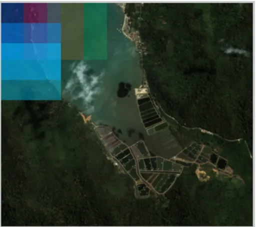
WV2’s high spatial resolution sensor has increased spectral sampling and range compared to QuickBird (4 bands) or IKONOS (4 bands) [5, 6, 7]. Although the ground sample distance (GSD) of the multispectral pixels is still two to three meters (depending on look angle), this combination of spatial and spectral resolution combined with an agile platform that can have fast revisit times is something new to the satellite remote sensing world.
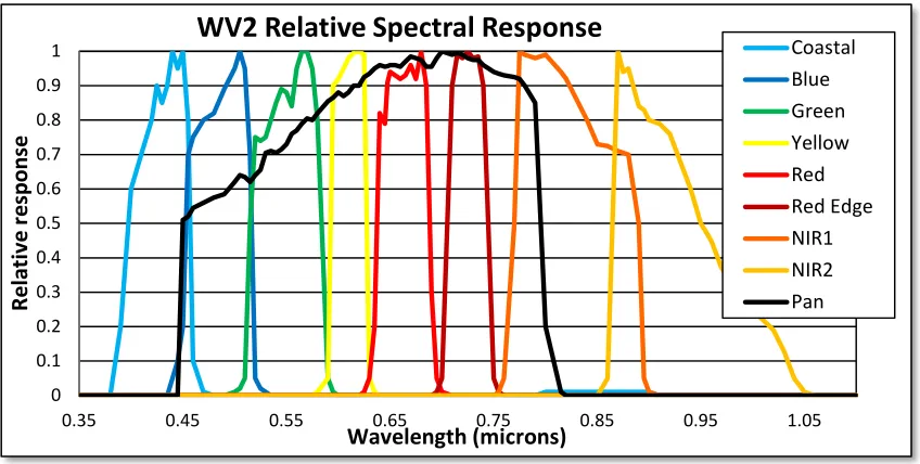
The increased spatial resolution and spectral resolution compared to previous platforms raise 0 0.1 0.2 0.3 0.4 0.5 0.6 0.7 0.8 0.9 1
0.35 0.45 0.55 0.65 0.75 0.85 0.95 1.05
Re la tiv e re spo ns e Wavelength (microns)
WV2 Relative Spectral Response
CoastalBlue Green Yellow Red Red Edge NIR1 NIR2 Pan
Figure 1: World View 2 relative spectral response. 3 of the 8 spectral channels have peaks in regions outside the high resolution panchromatic band’s response
Worldview-2 Characteristics
• High resolution
– 46 cm panchromatic at nadir
– 52 cm at 20° off-nadir
• 8 spectral bands (~0.4 - 0.9 μm)
– 1.84 m GSD at nadir (2.08 m at 20°)
• 1.1 day revisits at 1m GSD (assumed highly oblique)
• 3.7 day revisits at full resolution
• 16.4 km swath width
• Orbit: 770 km, 100 minute period, sun-synchronous
[image:21.612.77.501.71.285.2]• 6.5 m geo-location accuracy
5
several questions about the utility of such a sensor. In Figure 2 some detailed characteristics of the WorldView-2 platform are shown. With the increased number of narrow spectral bands, the sensor may characterize ground spectra accurately enough that techniques typically reserved for hyperspectral data could be utilized. Additionally, some of the new bands have specific characteristics that assist in a variety of applications. The coastal blue
band, for example, could provide utility to water studies, as the energy detected by such a band can penetrate further into water; the coastal band also allows the potential differentiation between two types of chlorophyll used to access vegetation health based on the spectral location of absorption features. The very high spatial resolution may enable the detection and identification of ground features typically only spectrally analyzed from aerial sensing platforms. Utilizing an agile platform, short revisit times could be exploited to introduce slow moving target tracking or near real time change detection.
Figure 3: Spectral and spatial resolution of several sensing systems. The resolution characteristics (left) of WV2 put it in a new region of the spectral/spatial space. The third dimension of this image system space is temporal resolution (right). Smaller font indicates higher spatial resolution.
Figure 3 shows the relative spatial and spectral resolution of several common sensing platforms. In addition, a third dimension can be included in that space based on the potential temporal resolution. Temporal resolution refers to the number of images per day. Based on the combination of increased spatial, spectral, and temporal resolution, this sensing platform can—with the help of improved algorithms—improve change detection and analysis beyond what has been available before. This research attempts to develop algorithms based on the characteristics of WV2, and applicable to many systems, that facilitate large area change analysis to identify and classify change areas and present them in
Space based hyperspectral
6
such a way that reduces the volume of information typically presented to an analyst for large area search.
Objectives
1.3
This research is undertaken to achieve one overarching objective, the development of methods for exploitation of multispectral multi-temporal imagery with the characteristics of the WV2 sensor. Further to this broad initial objective, the areas of change detection and clustering were chosen as the principal areas of interest for this research. Based on this main objective, several criteria for success are outlined below:
• Examine existing methods for change detection
utilizing multispectral imagery and determine their applicability to higher spatial resolution and spectral sampling.
• Research hyperspectral methods for change detection and determine their utility for WV2’s more coarsely sampled spectra.
• Develop new methods for change analysis tailored to the characteristics of WV2 type sensors.
• Develop new methods for automatic clustering based on atypical image data models.
• Combine existing and new methods in a robust and
fully automatic change analysis scheme for use on large area data sets.
7
Chapter 2:
Background
Historically, change detection has been approached with a large amount of analyst input [1, 8, 9]. While many methods have been developed, often simple image difference techniques are enough to lead the analyst in the right direction to manually measure the amount of change that occurred and what that change means. The difference maps are useful for large scale temporal imagery where the change identified could be used to task high resolution sensors to the area. Additionally, these approaches work best when the volume of imagery is such that it can be readily examined in a reasonable amount of time. With modern technology, the imaging response in situations where change detection would be needed (such as disasters like the 2010 Haiti earthquake) is so thorough that there is simply too much imagery over too large a physical area to be manually processed.
Large scale changes, on the order of tens to hundreds of meters, do not occur as frequently in nature as those on the order of one or two meters; for this reason, the large pixels of systems like Landsat tend to show change induced by human intervention or obvious large scale natural processes like flooding, forest fires, and seasonal change. This inherent likely cause of spatially small image changes (few pixels) seen in large scale imagery makes automatic change analysis on a small scale relatively unimportant. If an anomalous change occurs over several pixels where each pixel is 30m on a side, that change is almost certainly interesting to an analyst. Conversely, if the same number of pixel changes occur on a 2m scale, it is hard to say if the change is of interest or not. Because the high resolution of WV2 will lead to the identification of many more changes than low resolution systems, some automated methods are required to classify those changes.
8
Identifying Image Changes
2.1
The process begins with determining what parts of the change image are different than the base image. Many methods exist that can assist with this rudimentary change detection. Because this is the initial step in the process, the goal is to maximize change detection with reasonable risk for false alarms. Many methods for detecting change are outlined in the sections that follow. However, simply identifying change is not enough. Assigning a level of importance to the change found is the crux of a useful large scale automatic change detection process.
Figure 4: Example scene to scene changes. Are these shadow and illumination changes uninteresting or important?
9
and discriminate them are discussed in extended detail in section 4.2 , Cross image equalization.
Data Assumptions
2.2
Typically remote sensing data are assumed to fit a standard set of statistical and geometric models. The statistical model most used is the multivariate normal Gaussian distribution. This assumes that each material in a scene which is imaged is equivalent to a random per band sampling of a Gaussian distribution with the material’s expected value for a given band representing the mean of that distribution. This model has proven to be insufficient for characterizing a wide variety of scenes that contain a high level of clutter and a wide variability in materials and illumination conditions. High resolution multispectral image data does not always fit a Gaussian data model.
To combat this problem, many geometric models to represent the data have been introduced such as the linear mixing model. The linear mixture model makes the assumption that all pixels within a given subspace can be represented as linear combinations of the endmembers of a convex hull, and their constituent components can be extracted through un-mixing [8]. The endmembers are considered to be pure pixels of each material in the scene. While this method is not necessarily flawed, it makes the enormous assumption that pure pixels for each material imaged are identifiable in the scene. It also breaks down when illumination conditions vary drastically so that it is difficult to discern the spectrum of materials due to the lack of available light (such as in heavy shadow).
One goal of this research is to include methods that make a very limited number of data related assumptions and combine those methods with others based on the more traditional linear mixture, linear subspace, or statistical data model to create a robust multifaceted change detection scheme.
10
clustering methods, such as n-cuts (discussed below) and the later referenced Laplacian Eigen Maps (section 7.5.1) use a rotation to transform the data in such a way that planar cluster decision surfaces can be more successful. Spectral data can be thought of as filling a convex hull defined by the end members of the classes, or it can be thought to lie on a multidimensional manifold which is generally curled upon itself (representing cluster overlap and variability). If that manifold can be unfurled in the correct way, the spectral clusters will appear well separated and tightly grouped, easily distinguishable from each other.
Existing Methods
2.3
Change detection methods of interest for this research are widely varied. Because typical change detection research is targeted at very specific problems, there are few methods that apply themselves well to automatic large area change analysis. Existing techniques can be broken up into a few categories: those aimed at change on a large scale using LANDSAT data, methods targeted at high revisit rate such as change detection in video or low frame rate surveillance systems, hyperspectral image difference techniques, tile-based change detection, and object level change detection. Additionally, object level change detection techniques require a successful object identification or clustering step to achieve their results, so the clustering techniques known as k-means, ISODATA, normalized cuts, gradient flow, and Gaussian maximum likelihood are also of interest.
2.3.1 LANDSAT techniques
Land use studies are a common application for change analysis. Because of its long period of service and the readily available data, the thematic mapper (TM) aboard LANDSAT 5 and the enhanced thematic mapper (ETM+) on LANDSAT 7 are both widely used for change detection, and many algorithms have been written specifically for use with imagery from those systems. While many of these algorithms are not exclusive to LANDSAT data, they are particularly suited to the characteristics of the LANDSAT sensors. These techniques are certainly applicable to other imagery, but most fail because of the difficulty in registering high resolution imagery with sub-pixel accuracy.
2.3.1.1 Change vector analysis for vegetation change
11
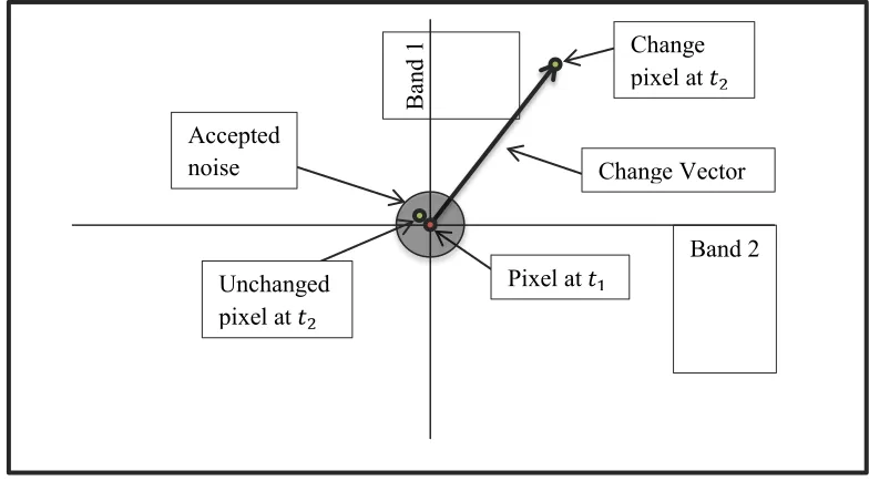
change vector. The intensity value of a pixel is compared, typically with the Euclidean distance, at time one and time two and a vector is drawn between them (see Figure 5). The change in the value is descried by a vector that is larger than some sphere of acceptable noise. For the analysis of vegetation change, Lorena [12] primarily used the work of Malila [10] to compare the “greenness” (G) and “brightness” (B) of LANDSAT pixels of the Brazilian Amazon forest. Creating change vectors from two composite bands allowed for four types of change to be identified. Increase in G with decrease in B indicated forest regrowth, decrease in G with increase in B indicated deforestation, and so on. This type of change analysis and classification is very effective on large pixels which can be accurately registered with sub-pixel precision and when the type of change being examined falls into a few specific and more importantly identifiable categories. For a high resolution large area change analysis problem, where the type of change is largely unknown, using change vectors to classify change is not feasible.
2.3.1.2 Secondary feature based methods (Vegetation index)
[image:28.612.128.520.454.671.2]LANDSAT has long been used to measure the vegetation index (VI) in large regions. The change in these vegetation indices can be used by simple image differencing to examine the change in certain regions. Singh [13] summarizes the use of the vegetation indices for change detection. The vegetation index is a band ratio to indicate vegetation health.
Figure 5: Change vector analysis example, demonstrating a changed and unchanged pixel.
Pixel at 𝑡1
B
and 1
Band 2 Change pixel at 𝑡2
Unchanged pixel at 𝑡2
Accepted
12
While the vegetation index differences are simple per pixel subtraction based methods, they represent a trend toward the classification of change, like the change vector analysis, which can be useful. This type of metric could be used on a tile level to produce a score to identify and classify the type of change that has occurred in the tile. Some types of vegetation change would be uninteresting salient change, like defoliation of deciduous trees in the fall, and others might be useful to present, such as deforestation.
Algorithms for low-resolution imagery all have the advantage that expected changes are land cover changes and will result in change in radiance that is very large compared to pervasive radiance changes [1, 13]. Although WV2 has a similar spectral composition, the vastly increased spatial resolution means that many techniques for LANDSAT will work poorly with WV2. Higher resolution leads to increased clutter and decreased effectiveness of examining the relative radiance change. LANDSAT is useful for finding comparatively large scale change; the small scale changes of WV2 scale will need unique methods to be properly identified.
The high resolution of WV2 detects such small ground objects that the scale of change which could be identified is altered drastically. So much, in fact, that pixel level methods become impractical for certain scene types. At a pixel level scale with one or two meter square pixels, small changes to single pixels can be so large that they wash out the detection of more subtle but larger scale change. The spatial resolution of the imagery limits the type of change that can be identified. Smaller changes can be identified in high resolution data, while large changes or more subtle ones are simply masked by the overwhelming number of small changes.
2.3.2 High temporal rate techniques
Certainly methods developed specifically for detecting small changes in high resolution imagery have been studied. However, these techniques are typically for very high temporal resolution (e.g. video) [14] or for identifying specific changes in a scene where very little has changed at all (e.g. finding a known target at a new location) [15]. These techniques generally are not designed to be applicable to unsupervised large area search.
13
others, describes the method of utilizing the temporal consistency of sequential images to eliminate the background and identify change. In general, these methods assume that each pixel should be modeled in time by a Gaussian distribution. By collecting all the samples for each pixel and computing their first order statistics, anomalous pixels can be identified by their distance to the overall distribution in time at each pixel location. A sequence of k
images, each with n pixels, is represented by a set of n Gaussian distributions with k points in each. Change is identified where pixel values are independent and no-change where they are dependent as expected.
Clearly this method relies on the exact registration of images and a large database of images to work with. While this type of change detection is successful for largely static surveillance video, it is only loosely applicable to satellite remote sensing. The combination of multiple base maps is likely to be necessary in satellite work, especially in change analysis of a frequently imaged region and similar techniques may be useful in the right scenario.
2.3.3 Covariance based image difference methods
Many well studied methods for change detection relate to image subtraction and pixel level comparison. The image difference is the per pixel subtraction of digital counts. This extremely simple technique can provide useful results if many criteria are met. The images would need perfect registration and very consistent illumination. To combat the shortcomings of the simple image difference, many more advanced techniques working on the same basic principle have been created.
2.3.3.1 Chronochrome
Shaum and Stocker created a method known as chronochrome [17, 18, 19] which has been applied to change detection [20]. The chronochrome method attempts to predict the linear transformation in the image data between two sensing situations based on the first and second order statistics of the data. The data from day one is used to predict what the data will look like if imaged under the same conditions as day two. Any deviation in this prediction is considered to be a change.
For a given data set where 𝑥𝑖 is a pixel in image one and the mean is subtracted so the expected value of 𝒙 is zero, the covariance is given by
14
Similarly, the second image is described by 𝒚 and the cross covariance is C =〈𝑦𝑥𝑇〉.Utilizing the notation of Theiler [20] to describe the anomalousness of a change pixel,
𝓐(𝑥,𝑦) = [𝑥𝑻𝑦𝑻]𝐐 �𝑥
𝑦� (2.3 .2)
where 𝐐is square symmetric and a function of 𝐗,𝐘, and 𝐂. All the covariance based change methods discussed will output a scalar value for each pixel representing the amount of change or anomalous change that is predicted to have occurred. This measure of anomalousness is given by the RX algorithm [21] for anomaly detection. To detect change, chronochrome utilizes an estimator for the values in the change image where the change image is assumed to differ from the base by a certain linear transformation, 𝑳. This estimator is based on the assumption that the pervasive change from one image to another is mostly linear and the change an analyst is looking for is non-linear and can be identified by finding the error in the estimator which is identified with the aforementioned RX method.
The linear transformation that minimizes the error in the estimator is found to be 𝑳= 𝑪𝑿−1 [20, 17]. The error is minimized because this method hopes to find small change in a large mostly unchanged scene. After implementing the method in a whitened space where
x�= 𝑿−𝟏𝟐x , (2.3 .3)
𝑪�= 𝒀−𝟏�𝟐𝑪𝑿−𝟏�𝟐, (2.3 .4)
and performing some additional equation manipulation, the projection matrix can be written as:
𝑸�𝒄𝒉𝒓𝒐𝒏𝒐𝒄𝒉𝒓𝒐𝒎𝒆 = �𝑰𝒙 𝑪� 𝑻
𝑪� 𝑰𝒚� −𝟏
− �𝑰𝒙 𝟎
𝟎 𝟎�. (2.3 .5)
The chronochrome technique also works in the opposite direction, from the change image to the base image. In that case the transform is 𝑳′= 𝑪𝑻𝒀−𝟏, and the projector becomes
𝑸�𝒄𝒉𝒓𝒐𝒏𝒐𝒄𝒉𝒓𝒐𝒎𝒆′ =�𝑰𝒙 𝑪� 𝑻
𝑪� 𝑰𝒚� −𝟏
− �𝟎 𝟎𝟎 𝑰
𝒚�. (2.3 .6)
15
For an agile wide-coverage space based multispectral sensor with 2-3 meter pixels, sub-pixel registration accuracy is not always guaranteed. The increased data from high resolution sensors for the same area coverage also calls into question the validity of a global covariance’s accuracy in describing the distribution for very large images. Furthermore, the decrease in spectral fidelity can limit the effectiveness of the covariance equalization. A poorer representation of the pixel spectrum, due to decreased spectral sampling and increased bandwidth, will lead to a poorer estimation of the linear transform between images. Additionally this method continues to utilize multivariate normal first order statistics to model data that often are poorly modeled by a Gaussian distribution.
2.3.3.2 Covariance Equalization
Recognizing that the requirement on sub-pixel registration was a boon to the chronochrome technique of calculating the cross covariance matrix directly, Schaum and Stocker developed the similar technique of covariance equalization [17, 19]. In covariance equalization, the estimator 𝑳 is designed to not contain the cross-covariance. Specifically,
𝑃=𝑌𝟏�𝟐𝑅𝑋−𝟏�𝟐 (2.3 .7)
where 𝑹 is an orthonormal matrix. In other words, its rows and columns are linear independent basis vectors of the subspace it describes. The choice of 𝑹 can depend on the imagery, but the authors indicate that the identity matrix 𝑰 works well [17]. The error in the transform and the anomalousness in that error are as follows:
error = y− 𝑃x (2.3 .8)
𝓐(x, y) = e𝑻〈ee𝑻〉−1e (2.3 .9)
16
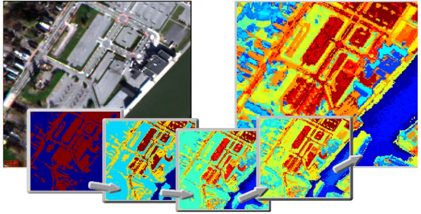
Figure 6: Example post classification change detection 2.3.4 Post classification change detection
Some change detection, known as feature based change detection, uses image features to identify change rather than pixel differences. These methods typically perform some type of feature classification or clustering and then compare the results between two images. This type of technique works well to identify interesting changes. Rather than simply indicating that change has occurred on certain pixels, these methods can identify new features or missing features or changing features. This type of method is straight forward to implement, assuming the feature classification process is successful. If two temporal images can be classified such that the classes represent the same materials, a class difference analysis can be used to identify change. Temporal data has also been used to improved classification, but these methods assume no change has occurred and are not of interest to change detection.
17
The results from this type of method are often the most useful, as the changes are not only identified but can be labeled based on the class they changed from and to [13, 22]. The various values in the class map difference image can be labeled to produce an output that displays specific types of change, i.e. deforestation, urbanization, new development, erosion, etc. A notional example of class-map based change difference images is shown in Figure 6. The difficulty with post-classification change detection is that is relies on high accuracy classification of two separate scenes. This is a daunting task with respect to wide area search or change analysis.
2.3.5 Tile based change detection
Recently research on tile based change detection, as opposed to pixel based methods, has increased. Tile based change detection is useful for large area change detection where the volume of information presented to an analyst can be significant and overwhelming. Recent work by both Ziemann et al. [23] and Schlamm et al. [24] has examined approaching change detection on a tile scale.
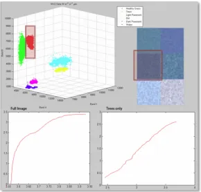
The work by Schlamm used the characteristics of the local point density of tiles in an image to identify change. The point density plot is a measure of the number of pixels that fit within a sphere in the hyperspace as that sphere increases in size. As the sphere grows the number of pixels within it grows as well, creating a monotonically increasing plot. This plot of number of pixels versus the volume of the sphere has a characteristic slope and tail length. In real image data the plots taper off asymptotically producing a tail. As the distribution of data becomes more multivariate normal, the tail length decreases. The tail is minimal for uniformly distributed data. Figure 7 shows a PDTL plot for the image pixels shown. When the plot is created for the nearly Gaussian tree class alone, the plot has an almost non-existent tail.
18
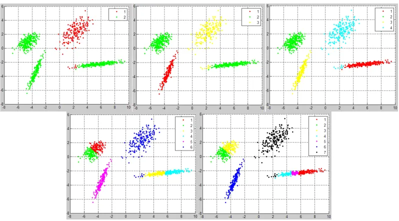
Figure 7: PDP plots for a six class image (top right) with the data shown (top left), for all 6 classes and for a single class (trees).
[image:35.612.143.433.73.351.2]The PDP plot is effectively a loglog plot of the cumulative histogram of the edge lengths from one pixel (the pixel nearest the mean) to every other image pixel. Other PDP plots are examined later based on different starting pixels (see section 4.5 Change metrics).
Figure 8: Example 𝚫𝑷𝑫𝑻𝑳 plot used to detect change.
19
scene content. The method utilized the square root of the determinate of the Gram matrix to calculate the volume of the n-parallelotope (in n-dimensional space) which contains the data. The Gram matrix of a set of 𝑘 vectors, 𝑣1,𝑣2, …𝑣𝑘, is a square symmetric matrix where each entry is the inner product described by
𝑮(𝒊,𝒋) = 〈𝒗𝒊,𝒗𝒋〉,𝒊,𝒋 ∈ 𝟏,𝟐, …𝒌 (2.3 .10)
The volume of the space is calculated for increasing dimensions until it reaches zero. The volume decreases as dimensionality increases; the simple example of the volume of a plane in three dimensions serves as an illustration to this possibly confusing statement. Once the third dimension, of length zero, is added to the multiplication, the total volume goes to zero as well. The monotonically decreasing volume as a function of dimension represents an estimate of the number of end-members needed to describe the scene, or loosely the number of end-member materials present in the scene. End-members are considered to be the vertices of the the n-parallelotope that encloses the data. Physically, an ideal end-member is a pure (un-mixed) pixel containing just one material, and one end-member would exist for each material in the image. Realistically, especially for cluttered scenes, true pure end-members do not exist for all scene containing materials. Change detection using the estimate of the volume is performed by finding changes in the peak magnitude of the volume estimate for a given image pair. Using this metric, a per tile change score can be calculated. Both methods, the Δ𝑃𝑃𝑃𝑃 and the Gram matrix volume estimate, described here could have application in the final large scale change analysis scheme outlined in this work.
2.3.6 Object level change detection
Another change detection technique is called object level change detection. Hazel [25] developed a methodology for utilizing an object identification system for change detection. The methodology he outlined worked by examining an image series to extract objects and features and to classify objects and associate them between scenes. To associate the objects a site model was initialized with the base image and subsequently updated as new or different objects were associated or identified to have changed. After the objects were associated, change detection was performed to identify new, moved, or missing objects.
20
be linked with each other between scenes or false changes will be identified. In his approach, Hazel identified a number of features about each object that could be used to associate them. For example, the center of the object’s position, the size of the object, and the overlap of their areas (across image 1 and image 2). After comparing these features, the change objects can be identified and presented as an anomaly change map. This object level change detection represents a part of the goal of this project: to provide information about what change is occurring rather than just change identification.
2.3.7 Clustering methods
For each of the last three techniques described above, an assumption is made that the imagery can be clustered or segmented successfully and accurately in one way or another. Many methods exist to cluster or classify spectral image data. Some of the most common methods include k-means and Gaussian maximum likelihood (GML), which represent automatic and supervised cluster respectively. Additional methods for automatic clustering which are of interest for this research are k-means [26], ISODATA [27], normalized cuts [28], and gradient flow [29, 30]. Automatic clustering is a requirement for any successful large scale approach to cluster or object level change detection. The supervised clustering of a high resolution image is tedious and infeasible for any large area approach that targets limited processing time for an end product. While often GIS information is used to aid in clustering, the methods of interest are data driven and attempt to cluster based only on the image data available, including temporal sets if available.
2.3.7.1 GML clustering
21
𝒈(x𝒊) =𝐥𝐧�𝒑(x|𝝎𝒊)�+𝐥𝐧�𝒑(𝝎𝒊)� (2.3 .11)
where 𝜔𝑖 represents the a priori class probabilities. Assuming that the data are modeled well by a multivariate normal distribution (thus the name Gaussian maximum likelihood) the conditional probability can be expanded to result in the following discriminate function:
𝒈(x𝒊) =𝐥𝐧�𝒑(𝝎𝒊)� −𝟏𝟐 𝐥𝐧(|Σ𝒊|)−𝟏𝟐(x− µ𝒊)Σ𝒊−𝟏(x− µ𝒊). (2.3 .12)
The discriminate function for each class is calculated for every pixel and the maximum of that function for each pixel is the class the pixel is assigned to. The latter half of the discriminate function contains the Mahalanobis distance, or statistical distance to the mean, which is why the GML classifier is sometimes referred to simply as the weighted Mahalanobis classifier (weighted by class probabilities). This supervised method, while using one of the more simplistic decision rules, is much more accurate that unsupervised methods at placing pixels into the correct cluster than, assuming the correct cluster is characterized by the training data (and that the data can be roughly modeled with a normal distribution). The assumption that each pixel is represented by the training data is not one to be taken lightly when working with large high resolution data sets with many regions containing unknown ground information. Supervised clustering, while not feasible for a fast large area clustering over an unknown region, can be well utilized as a benchmark for automatic clustering of a well-known scene.
2.3.7.2 K-means clustering
The k-means clustering method is an automatic method and is almost purely data driven. The method begins with a single user input (other than the image to be clustered), the estimated number of clusters (𝑘) within the scene. The k-means method then uses an iterative process to divide the data into the predetermined number of groups. First 𝑘
22
surfaces are linear, the k-means method works well to cluster scenes with few materials or large pixels, but for scenes with many small clusters and a high degree of image clutter, the method produces generally poor results due to the large overlap of clusters in the data space.
2.3.7.3 ISODATA clustering
ISODATA clustering is a near relative to k-means. ISODATA is given a range for the number of clusters rather than a single value and the algorithm is allowed to optimize the groups to the best value. After any iteration the ISODATA method can remove groups containing too few pixels or merge those with a high level of overlap. Additionally, clusters with too much within group variability can be split. ISODATA produces results very similar to k-means and in high clutter regions it tends to optimize to the upper limit of the user selected range. Generally speaking, especially in urban environments, there are typically far more reasonable spectral clusters in the data cloud than predicted by most human observers examining an image.
2.3.7.4 Normalized cuts segmentation
The normalized cuts segmentation process is typically utilized for color imagery rather than multi- or hyper-spectral. The method attempts to represent the image as a mathematical graph and utilize the graph adjacency matrix to iteratively segment the data. The methodology was introduced by Shi and Malik [28] in 2000. To represent the image as a graph, the authors used the simplest approach of creating an adjacency between each pixel to its two nearest spatial neighbors, specifically the pixel directly to the left and directly below the pixel of interest. Each of these edges was labeled in what is known as the graph adjacency matrix. The adjacency matrix is an 𝑛×𝑛matrix (for a set of 𝑛 nodes) with each entry, 𝐴(𝑖,𝑗), indicating the presence or lack of an edge between those two nodes with a one or a zero. The degree of a node (deg(𝑣𝑖)) is the number of edges incident with that node. This spatial creation of pixel adjacencies may work for a typical RGB picture of people or
23
scenery where adjacent pixels have a high probability of color similarity, but a more sophisticated approach for edge identification would need to be taken for aerial or satellite spectral imagery (such an approach is described in section 4.4 and 3.3 ). Further development of n-cuts has examined the use of other edge identification techniques and edge weighting functions [32].
Having established the 𝑛×𝑛 adjacency matrix, the matrix is manipulated to create what is known as the graph Laplacian. The normalized graph Laplacian is also an 𝑛×𝑛 matrix. Its entries are given by:
(2.3 .13)
Where 𝑣𝑖 and 𝑣𝑗 are vertices in the graph or image pixels. The image is segmented based on the signs the individual elements of the eigenvector corresponding to the second smallest eigenvalue of the Laplacian matrix. Each pixel is assigned to one of two groups depending on the corresponding sign of the eigenvector elements. Each group is then processed iteratively, starting with the creation of the adjacency matrix, until the desired number of segments is achieved.
While normalized cuts segmentation works well to identify regions in RGB imagery, they are generally spatially contiguous and much larger relative to the entire image than those that need to be segmented in remote sensing data. The normalized cuts method is difficult to implement for large multispectral imagery due to the inherent computational expense required to solve the full eigenvector problem to find the smallest eigenvectors of the very large Laplacian matrix. Additionally, the n-cuts method segments the image recursively with no mathematically defined stopping condition. The segmentation is also halted if the graph representation of the image has any disconnected components, which can occur if the adjacencies are determined spectrally rather than spatially.
2.3.7.5 Gradient flow clustering
24
connected to its 𝑘 nearest spectral neighbors based on the Euclidean distance. Pixels with many more than 𝑘 connections are in areas of high local density and by this method belong at the center of a cluster.
Figure 10 shows a representation of three clusters (upper left), and the graph when each pixel is connected to its six nearest neighbors. The bottom of Figure 10 shows the flow of the density gradient, with each pixel being assigned a direction of flow toward the center of its cluster. To calculate this gradient flow, a function is defined using the number of edge connections in the local area to represent the negative of the local density. The gradient flow is then constructed with the negative density acting as the sink and the cluster centers acting as the basins. The partial differential equation (PDE) system for the gradient flow of local density is iterated a number of times (user selected) to smooth the results so too many density centers are not defined. The goal is to define high density cluster centers rather than simply all points of high density. This smoothing influences the eventual number of clusters in the cluster map. In the PDE system, pixels are assigned a value of gradient flow indicating the density center to which they point and thus the cluster to which they belong.
[image:41.612.151.421.81.314.2]The gradient flow algorithm is a novel method because it requires no image specific input from the user other than the number of smoothing iterations; it defines the best number of clusters to use based on the density map of the image data. Additionally, the gradient flow
25
decision surfaces for cluster membership are non-linear and the method makes no assumptions about the inherent distribution of the data in the hyperspace. The method works well but does have difficulty in some scenarios and still outputs a single final cluster map.
Chapter summary
2.4
27
Chapter 3:
Topological Clustering
In addition to the overall goal of change characterization, and as a means to achieving it, automatic clustering was closely examined, and a novel method to perform clustering was developed. With the idea of utilizing topological methods to create a clustering based on data structure and pixel relationships, and automatic clustering methodology could be created without a reliance on statistical models.
Automatic image clustering and segmentation is an ongoing problem for imaging science, and is a method used in the feature based change analysis process. Clustering is the process of dividing an image into groups of pixels that identify the materials within the scene. The goal of clustering, as opposed to classification which attempts to label groups of pixels as specific materials, is to combine pixels with a certain level of spectral similarity [1]. Clustering typically assigns each pixel to a single group, although a subset of clustering methods known as fuzzy-classifiers use a probability to assign pixels to clusters rather than discrete labels. Most clustering is currently done with an analyst identifying sample regions and then finding all parts of an image that are similar enough to the training sample regions. This is supervised classification. Many supervised clustering techniques are very successful, such as Gaussian maximum likelihood, Gaussian kernel classification, neural networks, and support vector machines [1, 8]. One major difficulty in automating this process, especially for high spatial resolution imagery, is the variability in the number of classes or materials present in the scene and the time consuming aspect of identifying training regions.
28
At high resolution spatial scales, with pixels on the order or 1-2 meters, variations within what a human analyst may identify as a single material or class are extensive. One way to overcome this within class variability problem is to use a recursive classifier that identifies pixels within regions with increasing variability. If a clustering algorithm first identifies a large body of water and then currents, waves, or other inconsistencies within that body of water, this could be considered an improvement to the most wide-spread automatic classification methods in use today. If each region in a class map can be labeled as a sub-region of another larger sub-region then it becomes easier to interpret the relationship between automatically created regions.
Modularity clustering
3.1
The recursive method used in this research is based on the theory of the modularity of groups within networks. In social network theory, networks, represented mathematically with graphs, consist of nodes and edges. A node is just a point in any n-dimensional space and an edge connects two nodes. In graph theory self-connected nodes are possible, but in regard to image pixels, these have no physical meaning. To represent an image as a graph, it is necessary to visualize the image in an n-dimensional space, where n represents the number of bands in the imagery. Each pixel becomes a node, and edges can be drawn between pixels with a certain similarity or connectedness. There are 𝑛 nodes and 𝑚 edges in a graph. The number of connections (edges) incident with a node is the degree of that node. The degree of node 𝑖 is a scalar that counts the number of other nodes adjacent to node 𝑖. Now the adjacency matrix can be defined. The adjacency matrix 𝑨 is 𝑛 × 𝑛, and it has a zero at 𝐴𝑖𝑗 where nodes 𝑖 and 𝑗 are not adjacent and a one where they are adjacent. It is important to note that the edges are not an inherent part of imagery; they are drawn based on some metric to determine which pixels are similar enough to warrant an edge between them. The drawing of edges to turn a collection of pixels into a graph is a focal point of this method, and the success of this edge creation determines the success of the later separation of the graph into regions/classes.
29
Another method is to perform a nearest neighbor search using some knowledge of the structure of the data. Many different algorithms exist to preprocess data sets for fast nearest neighbor searches. The fast nearest neighbor search using the ATRIA tree structure [33] is one such method which is well known and straightforward to implement.
The fast k-nearest neighbor search (KNN) method utilizes a tree structure of the data known as ATRIA. ATRIA is a triangle inequality based algorithm [33]. The ATRIA structure is essentially a loose clustering of the data by recursively splitting the data around a central point within each cluster. At each level of the ATRIA tree, each point is present in only one cluster. The actual nearest neighbor search is accelerated using the ATRIA structure because only a certain portion of the clusters need to be searched to find the k nearest neighbors of a given pixel. Only rarely will a point have neighbors outside the cluster being searched and require additional time to locate the neighbor.
To prune the results of the KNN search to increase the quality of the edges drawn, several methods are implemented. For any given pixel, the k nearest neighbors will likely include some pixels which are quite similar to the pixel and some which are simply close enough to be among the k nearest neighbors but not close enough to belong to the same overall cluster. The edges drawn to those pixels are poor edges and therefore must be limited. To limit these edges a threshold is used related to the expected distance of the pixels. Edges which are greater than a certain (tunable) percentage of the mean edge length for a given pixel’s k-nearest neighbors can be discarded. More issues concerning edge creation and pruning will be addressed later on.
Figure 11: Example of edge creation and clustering in n-D space. Each pixel (node) is connected (adjacent) to its 2 nearest neighbors.
Band 2
Band 1
2-NN Graph
Band 2
30
In Figure 11, each dot represents a pixel or node in the data. Each pixel is connected to its two nearest neighbors. Because a given pixel could be one of the two nearest neighbors of many pixels, some have more than two edges. The number of pixels in a group with more than k edges is an indication of the density of pixels in that group.
Once the image has been represented as a graph, the modularity of that graph can be used to split it into two or more sub-graphs. Modularity is a measure of the difference between the number of edges within a selected group of pixels and the number of edges expected in a random group with the same degree distribution [34, 35, 36]. Newman defines a vector 𝑠, where the vertex 𝑖 belongs in group one if 𝑠𝑖 = 1 and in group two if 𝑠𝑖 = −1. Modularity,
𝑄, is described as
𝑄 =41𝑚 � �𝐴𝑖𝑗 −𝑘2𝑖𝑚 � 𝑠𝑘𝑗 𝑖𝑠𝑗 𝑖𝑗
. (3.1 .1)
where 𝑚, is the total number of edges, 𝑨is the adjacency matrix of the graph, and 𝑘𝑖 is the degree of node i. The adjacency matrix will be sparsely populated; although its 𝑛×𝑛 size could be a memory burden, a sparse implementation makes it manageable. Equation (3.1 .1)
can be simplified by converting to matrix form where it becomes
𝑄 =41𝑚 𝒔T𝑩𝒔 , (3.1 .2)
and where
𝐵𝑖𝑗 =𝐴𝑖𝑗−𝑘2𝑖𝑚𝑘𝑗. (3.1 .3)
31
modularity matrix. Although n-cuts splits based on an eigenvector of a matrix derived from the adjacency matrix, the modularity requires the identification of the largest eigenvalue rather than the smallest and therefore allows for much faster processing of very large datasets using the power method to find the necessary eigenvector.
To separate a graph into more than two groups, Newman cautions against simply removing the edges and recalculating the modularity eigenvector [34]. This note of caution is applicable when the graph contains preexisting edges. In this application, the graph is a variable association of pixels in an image. The edges drawn between pixels are chosen and not an inherent part of the image. Because the image pixels are not part of a pre-defined graph, using modularity with imagery allows for additional flexibility to redraw the graph without changing the network. It is simple and practical to redraw the graph for each group of pixels and run the modularity algorithm from the beginning. This technique leads to the best split for each possible subset of pixels. The distribution of edges could be very different for the graph representing a given subset of pixels than it was previously as a sub-graph of the full set of pixels. Using a new graph instead of the existing arrangement at each level yields the best split.
It is an important distinction between modularity and other common automatic clustering methods that the modularity technique makes divisions of the pixels recursively with non-linear decision surfaces. For each split the decision surface is defined based on the maximal modularity of the graph that was created to represent the pixels in that group. The decision surfaces are unrestricted and can take any shape.
32
Figure 12: An example output of group splitting with modularity. Each cluster can be labeled with a unique identifier that indicates the path it took through the various splits; additionally, a quality score for each split can be maintained.
The fully un-supervised modularity technique uses some simple stopping criteria to prevent over clustering. First, the character of spectral imagery and the knowledge of the scene content can be used to define a smallest group size for which a split will be attempted. This group size threshold does not limit the size of the smallest clusters, but instead limits the size of the smallest group for which an additional split will be attempted. This simple size threshold supersedes the modularity parameter discussed below. In real imagery the analyst may be uninterested in any clusters smaller than a certain level, and the simple group size threshold will limit clusters of such a size. In much of this research groups with less than 3-5% of the total image pixels are not split another time.
For the second parameter a threshold for 𝐐 is used. Only splits that produce a 𝐐 value greater than a certain threshold are allowed. Based on testing by this author and reported in the literature related to the development and verification of modularity for networks, the threshold for 𝐐 for a good quality split is 0.4. A value above 0.35, for a relatively small group of pixels, is still a reasonably good split. However, for very large networks, on the order of 100,000 nodes, these values break down. At a level near a large sized image on the order of 10 million nodes the thresholds break down. The best approach is to limit the split based on the modularity only for groups smaller than some reasonable percentage of the total image. This adjustable parameter should be set at some initial value, and then scaled based on the size of the group being split. Based on images ranging from 100x100 to 1000x1000 pixels, threshold values near 0.35 have worked well in this research to limit over-clustering in real
Group 1
1, a 1, b
1, a, i 1, a, ii 1, b, i 1, b, ii
1, b, i, A 1, b, i, B 1, b, ii, A 1, a, ii, B
33
imagery. However, the threshold should be dramatically lowered, by a factor of 4 for example, for groups containing more than half the total image pixels. The threshold works best with the images tested as part of this research when it varies quadratically
![Figure 10: Gradient flow, reproduced from Basener [30].](https://thumb-us.123doks.com/thumbv2/123dok_us/48353.4419/41.612.151.421.81.314/figure-gradient-flow-reproduced-basener.webp)