An Integrated Multiperiod OPF Model with
Demand Response and Renewable Generation
Uncertainty
W. A. Bukhsh,
Member, IEEE
, C. Zhang,
Member, IEEE
, P. Pinson,
Senior Member, IEEE
Abstract—Renewable energy sources such as wind and solar have received much attention in recent years, and large amounts of renewable generation are being integrated into electricity networks. A fundamental challenge in power system operation is to handle the intermittent nature of renewable generation. In this paper, we present a stochastic programming approach to solve a multiperiod optimal power flow problem under renewable generation uncertainty. The proposed approach con-sists of two stages. In the first stage, operating points of the conventional power plants are determined. The second stage realizes generation from the renewable resources and optimally accommodates it by relying on the demand-side flexibilities. The proposed model is illustrated on a 4-bus and a 39-bus system. Numerical results show that substantial benefits in terms of re-dispatch costs can be achieved with the help of demand side flexibilities. The proposed approach is tested on the standard IEEE test networks of up to 300 buses and for a wide variety of scenarios for renewable generation.
Index Terms—Demand response; optimal power flow; power system modelling; linear stochastic programming; smart grids; uncertainty modelling; wind energy.
NOMENCLATURE
Sets
B Buses, indexed byb.
L Lines (edges), indexed by l.
G Generators, indexed by g.
W Renewable generators, indexed by w.
D Loads, indexed byd.
D0 Flexible loads, D0⊆D.
Bl Buses connected by linel.
Lb Lines connected to busb.
Gb Generators located at bus b.
Db Loads located at bus b.
S Scenarios, indexed by s.
The authors were partly supported by Danish Council for Strategic Research through the projects PROAIN (no. 3045-00012B/DSF), iPower (DSR-SPIR program 10-095378) and 5s - Future Electricity Markets (no. 12-132636/DSF)
W. A. Bukhsh is with the Institute of Energy and Environ-ment, Department of Electronic and Electrical Engineering, Univer-sity of Strathclyde, 204 George Street, Glasgow G1 1XW, UK (e-mail:
C. Zhang and P. Pinson are with the Department of Electrical Engineer-ing, the Technical University of Denmark, Building 358, 2800 Kgs. Lyngby, Denmark (e-mail:{chzh, ppin}@elektro.dtu.dk)
T Discrete set of time intervals, indexed byt.
TF
d Flexibility windows for demandd,T
F
d ⊂T×T. Parameters
bl Susceptance of linel.
τl Off-nominal tap ratio of linel. PG−
g ,PgG+ Min., max. real power outputs of con-ventional generatorg.
PD
d,t Real power demand of loadd. fg,t(pGg,t) Cost function for generatorg. PW
w,t Initial forecast for real power generation availability from generator w in time
periodt.
∆PwW,s,t Change in generation availability under scenario s from generator w in time periodt.
λw,s Probability of scenarios.
CWw,t Cost of renewable generation spillage. Fd−,t,Fd+,t Min., max. load flexibility of demand at
busd.
∆Pg−,t,∆Pg+,t Min., max. change in operating point of generatorg during time period [t,t+1].
Rg−,t,R+g,t Min., max. regulation of generatorg. CR−
g,t,CRg,+t Downward, upward regulation cost for generatorg.
CD−
d,t,C D+
d,t Cost of decreasing, increasing demand in the time periodt.
Plmax Max power flow capacity of linel.
Variables
pGg,t Real power output of generatorg. ∆pG
g,s,t Second stage recourse variable for real power output of generatorg.
∆pG+
g,s,t, ∆pG-g,s,t Upward, downward regulation variables for real power output of generatorg. pW
w,s,t Real power output of renewable gener-atorw.
pL
l,s,t Real power injection at busbinto linel (which connects buses bandb0). pD
d,s,t Real power delivered at busd. αd,s,t Proportion of load delivered at busd. α+
d,s,t, α−d,s,t Variables for increase, decrease in de-mand supply at busd.
Acronyms
(M)OPF (Multiperiod) optimal power flow. (S)UC (Stochastic) unit commitment.
RES Renewable energy sources. TSO Transmission system operator.
DSO Distribution system operator.
LMP Locational marginal price. ILC Interpretable load control.
DR Demand response.
I. INTRODUCTION
E
LECTRICITY networks around the world are expe-riencing extensive changes both in operations and infrastructure. These changes are primarily driven by the liberalization of electricity markets and our increased fo-cus on eco-friendly generation. Large-scale renewable en-ergy sources (RES) are encouraged by different incentive schemes to meet government policy goals on climate re-lated issues. Managing and operating a power system with considerable penetration of RES is a challenge and many countries are investing substantial resources in planning and expanding current infrastructure to cope with RES integration. Wind power generation is the most widely used source of renewable energy and it has been integrated into many power systems around the world [1], [2], while solar power is catching up at a rapid pace.The non-dispatchable nature of wind power introduces additional costs stemming from the management of inter-mittency [3], [4]. Extra reserves are required-at an additional cost-to hedge against the uncertainty from the partly pre-dictable wind power generation. Despite the advancements in forecasting methodologies and tools, the hour-ahead forecast errors for a single wind farm may be on average as high as 10%-15% of its expected output [5]. The effects of these forecast errors are expected to become more pronounced in future as the share of RES increases in power networks.
In contrast, the demand at a transmission level has a large base component that can be predicted accurately. In power systems optimization problems, electricity demands are typically modelled as inelastic. In reality a substantial amount of the electricity demands are elastic [6]. Electric demands such as plug-in electric vehicle (PEV) charging, district heating and heating ventilation and air condition-ing (HVAC) systems are elastic demands that constitute a considerable percentage of the total demand,e.g.more than one third of the US residential demand is flexible [7]. The
majority of these demands aredeferrablemeaning that part of a demand can be shifted in time while respecting the deadlines and ramp-rate constraints [6].
Demand response (DR) is a way to utilize electricity demand as a resource to increase efficiency and reliability of an electricity network [8]. Demand response is an active area of research and there is a vast amount of prior work in this domain (e.g. see [9] and references therein). Demand response is generally characterized as price-based DR and incentive-based DR [10]. Demand response programs are generally managed by the distribution companies (DSO) or entities other than the transmission system operator (TSO). Most if not all of the current literature focusses on price-based DR while modelling transmission level optimization problems [9], [11]–[14]. The practicality and benefits of such optimization models incorporating price-based DR are not very clear, especially in view of reliability and volatility of power systems [15]. In this paper we revisit the multi-period optimal power flow problem and propose a two-stage stochastic model that incorporates demand as a flexible asset, the uncertainties in generation from the RES and consideration of an objective of total cost of generation minimisation. The following two subsections give an overview of the relevant literature and contributions of this paper, respectively.
A. Literature review
Traditional formulations of the OPF problem have been extended to account for the variable and partly-predictable nature of wind power generation [3], [16]–[18]. These papers capture the intermittent nature of wind power generation using different probabilistic techniques and determine a robust operating point of conventional generating units to meet a constant demand. With stronger focus on the de-mand side, authors in [19] consider dede-mand-side participa-tion as well as uncertainty in the demand bids. An optimal bidding strategy for an aluminium smelter in the day-ahead markets is developed in [20]. The market prices for day-ahead are treated as stochastic variables and the proposed model determines the optimal spinning reserve provision as well as the power consumption of an aluminium smelter. Authors in [21] extended the optimal power flow problem to a two-stage stochastic optimization problem: the first stage of the problem is to find a steady-state operating point for the large generation units while the second stage of the problem is to schedule more expensive fast-response generation units. The uncertainty in renewable generation is captured by using a set of scenarios; demand is assumed to be deterministic and the problem is not time coupled. This means that the optimal operating point is independent of the temporal characteristics of the system.
t1 6 t2 12 t318 t4 24
0.6 0.7 0.8 0.9 1
t (hr)
T
ot
al
D
eman
d
(N
or
maliz
e
d
)
P
[image:3.612.56.292.48.230.2]PdD: Total demand Demand Flexibility
Fig. 1. Flexibility in an aggregated demand. Total demand should be conserved in the time windows [t1,t2] and [t3,t4].
present a stochastic optimization framework for day-ahead operation of a electricity network. Their model includes unit-commitment, (N-1)-security constraints and a model of electricity storage. Flexible demands are modelled as dispatchable loads, which means that a demand can be shed at a price.
Much of the relevant work in this area focuses on either modelling of the uncertainty in renewable generation or modelling of the demand response. To the best of our knowledge, there are very few papers which deal with both of these aspects in a generic framework. Authors in [23], [24] have also alluded to the sparse literature on the problem.
B. Contributions of this paper
We present an optimization model that considers the flexibility offered in demand bids from the DSOs and optimally utilizes this flexibility by minimizing the total cost of generation. We propose that the DSOs embedded within a transmission network provide inelastic demand bids along with a flexibility interval; this means that the demand bids are elastic to a certain level. Such flexibility can be achieved by a DSO’s own DR programs. Fig. 1 shows a possible scenario of such a flexibility on an aggregated demand from a single DSO. If such information is available to a TSO then the decision problem is to optimally utilize the generation from RES while utilizing the flexibilities of the demands.
The main contributions of this paper are twofold:
• a revisited multi-period OPF formulation with
inte-grated demand response and renewable generation uncertainty;
• a rigorous mathematical model of demand response.
In contrast to recent approaches, we give a complete mathematical model of the demand response and also for-mulate the constraints for considering the demand shift and the conservation of demand for a given time period. In spite of its generality, the proposed model is computationally efficient and the approach holds promise. The proposed
approach can also be used as a tool to project future LMPs given the demand side flexibilities. The projected prices are useful information for the distribution companies, and they can use this information to plan their demand response strategies [10]. Finally we provide the wind scenarios and the network data of all the numerical results presented in this paper in an online archive at [25].
The remaining sections of this paper are outlined as follows. Section II gives the formulation of the problem. Numerical results are given in Section III and the conclu-sions are given in Section IV.
II. PROBLEMFORMULATION
In this paper, a two-stage stochastic formulation is pre-sented in a deterministic equivalent form [26]. In the first stage, decisions are made about the dispatch from the conventional generators. The second stage realizes the generation from the RES. Any resulting supply-demand mismatch is alleviated by the DR and slight adjustments of the operating points of the conventional generators. We assume that the DSOs can bid demand along with the flexibility for each time interval in a given time horizon. The transmission system operator can either meet the demand or can use the flexibility (by paying a price) to accommodate the uncertainty from the RES.
Consider a power network with the set of busesB. LetW denote the set of renewable generators in the network. Since the real power generation from the renewable generators is uncertain, let S be the set of real power generation scenarios of these generators. LetG be the set of conven-tional power plants andT :={1, 2,· · ·,T} be the set of given time horizon. In the following, we give the constraints and objective function of our two stage stochastic multiperiod OPF problem.
A. Power flow
Let pGg,t be the real power generation from the conven-tional generatorgin the time intervalt. The power balance equations are given as,∀b∈B,s∈S,t∈T:
X
g∈Gb
³
pGg,t+∆pGg,s,t´+ X
w∈Wb
pWw,s,t= X
d∈Db
pDd,s,t+ X
l∈Lb
plL,s,t (1) where pW
w,s,t denotes the real power output taken from the renewable generator w, pDd,s,t denotes the real power delivered to the demand d and pLl,s,t is the flow of real power in the line l in the time period t in the case when scenario s is realized, respectively. The power flow equations are given as,∀l∈L,s∈S,t∈T:
plL,s,t= −bl
τl
¡
θb,s,t−θb0,s,t¢ (2)
variables∆pGg,s,t in (1) are modelled in terms of the upward and the downward regulation variables as follows:
∆pGg,s,t=∆pG+g,s,t−∆pG-g,s,t (3a) 0≤∆pgG+,s,t≤R+g,t (3b) 0≤∆pgG-,s,t≤R−g,t (3c) whereRg+,t, Rg−,t are the permissible upward and downward regulation of the generator g in the time period t, respec-tively.
B. Demand Model
Let D denote the set of real power demands and we assume that a distribution network is attached to each bus d ∈D. Demand at the distribution network is aggregated and is denoted by PdD,t. We assume that each distribution company at the demand busdknows about the flexibility of their demand during the time intervalt. This flexibility can either come from a distribution company’s direct control over some demands or from its DR programs.
Letαd,s,t be proportion of the load delivered at busd at the time period t for the scenario s. Let [F−
d,t,Fd+,t] be the flexibility interval of the demand at bus d and at the time period t. The flexibility interval is defined aroundαd,s,t= 1 and therefore we have 0≤Fd−,t ≤1 and Fd+,t≥1. If the demand at bus d is not flexible then F−
d,t =Fd+,t=1 are used. If the demand at busd is flexible then it is placed in the set D0⊆D.
The demand model is given by the following set of constraints:
pdD,s,t=αd,s,tPDd,t (4a) 0≤Fd−,t≤αd,s,t≤Fd+,t (4b) αd,s,t=1,∀d∈D\D0 (4c)
where (1−F−
d,t) and (Fd+,t−1) are proportions of the demand d which can be decreased or increased in the time interval t, respectively.
1) Cost of the demand response: We introduce two pos-itive continuous variables α+d,s,t, α−d,s,t that give the p.u. increase and decrease in the amount of real power delivered to the demand bus d, respectively. These variables are modelled linearly as:
αd,s,t =1+∆αd,s,t (5a) ∆αd,s,t=α+d,s,t−α−d,s,t (5b) 0≤α+d,s,t≤Fd+,t−1 (5c) 0≤α−d,s,t≤1−Fd−,t (5d) LetCdD+,t andCdD-,t be the cost of upward and downward regulation of the demand d during the time interval t, respectively. The cost of the demand response for a single time period is given by (CdD+,tα+d,s,t+CdD-,tα−d,s,t)PdD,t. Since the cost of upward/downward regulation is strictly positive and one of the objectives in our optimization problem is
to minimize the cost of demand response, at an optimal solution both the upward and the downward regulation variables for a demand cannot be nonzero. For example, if an optimal decision is to increase a demand at busdby 10% during a time periodt then the optimal decision variables would take up the valuesα+
d,s,t=0.1 andα−d,s,t=0.0 with the cost of 0.1CdD+,t. A feasible solution for this situation could be α+
d,s,t =0.2 and α−d,s,t=0.1 but then the cost of this solution is 0.2CdD+,t+0.1CdD-,t which is obviously higher than the optimal solution cost of 0.1CD+d,t.
2) Conservation of the demand: If a demand at a busd is flexible in the time window [ts,tf] and it is required that the total consumption over a time period is kept constant then this situation can be modelled using the following linear equations: ∀d∈D0, [ts,tf]∈TdF={[ts,tf] :ts,tf ∈T,ts< tf}:
tf
X
t=ts
pdD,s,t= tf
X
t=ts
PdD,t (6)
whereTdFis the set of flexibility windows for the demand at busd. For example in Fig. 1 we have TdF={[t1,t2], [t3,t4]}.
The optimization would decide the amount of the de-mand to be consumed in each time interval. Note that we assume that there is enough power to support a task that requires more than one time interval to finish. This assumption is justifiable because of the lower bound on the value of αd,s,t. We also assume that the flexibility can be utilized in any way across the time intervals. In practice the flexibilities depend on the type of demands, e.g. for some demands we may need to consider constraints on up and down times, charging/discharging rates, etc. All these technical details can be modelled using linear constraints. However technical details and discussion on the subject are beyond the scope of this paper.
C. Operating constraints
Generation from the conventional generators is bounded by the following inequality constraints:
PgG-≤pGg,t+∆pGg,s,t≤PgG+ (7) wherePgG-,PG+g are the lower and the upper bounds on the generation output of the generator g, respectively.
It is not possible for a conventional generator g to considerably deviate from its current operating point in short time scales [21]. Therefore we limit the amount of change in the generation depending on the ramp rate of the individual generators. The ramp rate constraints are given as:
∆Pg−,t≤pGg,t+1−pgG,t (8a) pgG,t+1−pgG,t≤∆Pg+,t (8b) The line flow limits are given by the following set of constraints: ∀l∈L,t∈T,s∈S:
where Pmax
l,t is the real power capacity limit of the linel. D. Scenarios for the RES
Forecasting of renewable energy generation is a very active area of research, especially for wind and solar energy applications. While forecasts were traditionally provided in the form of a single-valued trajectory informing of the expected generation for every individual lead time and location of interest, emphasis is now placed on probabilistic forecasts in various forms [28]. For decision problems where the space-time dependence structure of the uncertainty is important, forecasts should optimally take the form of space-time trajectories.
In this paper, scenarios of the wind power generation are used as input to the stochastic programming approach to solve the proposed problem. The exact setup, data and methods of [28] are employed. A sample of 100 space-time scenarios are generated which will be used for the simulation of results. The scenarios are made available online at [25].
In our simulations we assume zero cost of generation from wind power [29]. Moreover wind power from the source w in the time period t can be spilled continuously to zero at the price ofCwW,t. LetPwW,tbe the initial forecast of power generation availability and let∆PwW,s,t be the change in the generation availability corresponding to the scenario s for the generator w in the time period t, respectively. The wind power output for the generator wis modelled as follows:
0≤pWw,s,t≤PwW,t+∆PWw,s,t (10) E. Objective function
Let λw,s be the probability of the scenario s for the renewable generator w. The objective is to minimize the cost of generation from the conventional generators, and optimally utilize the generation from the RES while initi-ating the demand response from the distribution system operators. Note that we do not consider ramping cost of the generators between the time intervals. Overall the objective function is to minimize the following, over the given time horizon:
z= X
g∈G
f(pGg,t)+X
s∈Sλ
w,s
X
w∈W CWw,t¡
PWw,t−pWw,s,t¢
| {z }
Cost of wind spillage
(11)
+X
d∈D ³
CdD+,tα+d,s,t+CdD-,tα−d,s,t´PdD,t
| {z }
Cost of demand response
+X
g∈G ³
CR+g,t∆pG+g,s,t+CR-g,t∆pG-g,s,t´
| {z }
Cost of generation regulation
1 2
3 4
∼
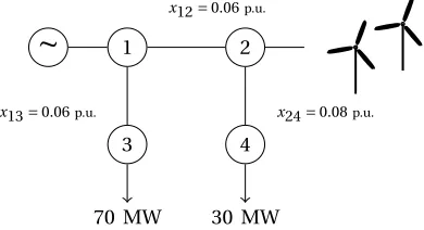
70 MW 30 MW x12=0.06p.u.
[image:5.612.339.534.55.161.2]x13=0.06p.u. x24=0.08p.u.
Fig. 2. 4 bus network, with a conventional generator at bus 1 and a wind farm at bus 2.
6 12 18 24
0.5 1
t (hrs)
P
W w,
t
(p
.u.)
Initial forecast Scenarios
Fig. 3. Initial forecast and 20 scenarios for wind power generation at bus 2.
F. Overall formulation
The overall formulation of the problem is given as fol-lows:
minX t∈T
z³pGg,t,pWw,s,t,αd,s,t,∆pGg,s,t
´
(12a)
subject to
(1−10) (12b)
Depending on the objective function f(pGg,t), the overall problem is then linear or quadratic program (LP or QP). We use CPLEX 12.06 [30] called from an AMPL [31] model to solve the problem.
In principle, other physical and operational constraints such as spinning reserve requirements can be included in the current formulation, and the solution approach that we describe here remains valid.
III. NUMERICAL EXAMPLE
A. An illustrative example: 4 Bus Case
Consider a small 4 bus network as shown in Fig. 2. The network consists of a generator at bus 1 and a wind farm at bus 2. Total demand in the network is 100 MW. Complete data for this network is available online at [25].
[image:5.612.317.557.200.348.2]0 10 20 30 40 50 10
12 14 16 18
Wind Penetration (%)
C
ost
of
g
ener
ation
($
M
Wh)
±0% Flexibility
±10% Flexibility
±20% Flexibility
[image:6.612.56.291.54.191.2]±30% Flexibility
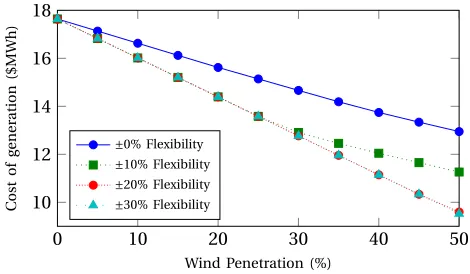
Fig. 4. Generation cost vs wind power penetration for 4 bus network.
The marginal price of the conventional generator at bus 1 is a monotonically increasing quadratic function of the real power generation. We assume the cost of wind spillage to be unity and the ramp rate of the generator at bus 1 to be
±10%. It is important to note that if there is no flexibility in the demand, the ramp rate of the generator at bus 1 should be equal to or greater than the maximum rate of change in the demand during any given time interval to ensure the feasibility of the optimization problem.
The regulation cost of the generator at bus 1 is assumed to be CR+
1,t=1.4>0.8=C1,R-t. We further impose the con-straint that the total demand should be conserved over the given time horizon and the cost of the demand response is considered to be CdD+,t=CdD-,t=0.5. Fig. 4 shows the cost of generation as a function of wind power penetration in the system. We can observe a general trend that the cost of generation is monotonically decreasing as the wind power penetration in the system is increased. This follows from the fact that we have assumed zero cost of generation from the wind. Even if the cost of wind power generation is non-zero, it is much less than the cost of conventional power generation and hence this assumption is justifiable. Further we note that when there is no flexibility from the demand, uncertain wind power generation can only be managed by adjusting the generator outputs in the second stage of the problem. As the wind power penetration is increased in this case, more wind is spilled because the generators cannot be regulated cheaply and rapidly to accommodate the variations from the wind power. The cost of generation decreases when the demand is made more flexible. There is no difference in the cost of generation between ±20% and
±30% demand flexibility. This is because of the fact that tapping on demand as a resource is no longer economical. For this example we can say that for the given ramp rate of
±10% and for the given RES scenarios, the optimal demand flexibility needed to fully utilize the wind power is±20%.
We have used scenarios to capture the uncertainty in the generation from the RES. Increasing the number of scenarios results in more accurate modelling of the stochas-tic process. Fig. 5(a) shows the difference in the cost of generation when scenarios are increased from 20 to 100. The difference in the cost of generation between 20 and 100 scenarios increases as the wind penetration in the system
0 10 20 30 40 50 0
2 4 6
Wind Penetration (%)
D
iff
er
en
ce
in
g
e
n
er
ation
cost
s
(%)
±0% Flexibility
±10% Flexibility
±20% Flexibility
±30% Flexibility
(a) Value of Stochastic Solution (20 scenarios vs 100 Scenarios).
0 20 40 60 80 100 0.8
0.85 0.9 0.95 1
Number of scenarios
N
or
maliz
ed
c
ost
of
gen
e
rat
ion
[image:6.612.328.550.56.186.2](b) Robustness of stochastic solution.
Fig. 5. Robustness of the solutions of 4 bus network with respect to uncertainty in the wind power generation.
increases. The difference between the cost of generation for given demand flexibilities and penetration levels, is always less than 6% (corresponding to a 400% increase in number of scenarios). Fig. 5(b) shows the monotonically increasing trend of generation cost as the number of scenarios is increased. We note that the curve in Fig. 5(b) smooths off as the number of scenarios is increased, which shows that after a certain point including more scenarios will not have any significant effect on the optimal solution.
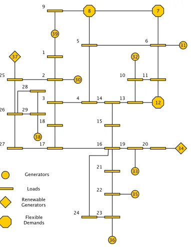
B. 39 Bus Case
Consider the 39 bus New England test network obtained from [32]. This test network consists of 39 buses, 10 gener-ators, and 46 transmission lines. We modify the network as follows. We consider 8 conventional generators, and two renewable generation sources at the buses 34 and 37, respectively. Demands at the buses 7, 8 and 12 are considered to be flexiblei.e.,D0={7, 8, 12}. The topology of
the network is shown in Fig. 6. The default data from [32] assumes same cost of generation for all of the generators. We take more realistic generation cost data from [33] to use in our simulations. The modified data of this network is available at [25].
Fig. 6. Modified 39 bus system with 8 conventional generators, 3 flexible demands, 18 inflexible demands and 2 renewable generators.
network is 7367 MW, and approximately 15% of the total capacity is from the renewable generators at the buses 34 and 37. We assume that the ramp rate of all the conventional generators is ±5%. The cost of the generator regulation isCgR+,t=1.8,CgR-,t=0.5, ∀t∈T,g∈G.
We further impose a constraint that the demand at the flexible bus 8 is conserved between the time intervals [4, 8]. The cost of using demand flexibility isCdD+,t=1.1,CdD-,t=0.7 for all the demand buses except for bus 8 where the cost when demand is conserved is C8,D+t =C8,D-t=0.5, 4≤t≤8.
Fig. 7 shows the result of our model on the 39 bus case as the flexibility of the demand is increased. Line limits were not active at the optimal solution, therefore the locational marginal prices at all the buses were equal. The solid (blue) line shows the results when the demand at buses 7, 8 and 12 are not flexible. In this case the marginal prices follow the behaviour of the demand curve,i.e.the prices are high when the demand is high and the prices decrease with the decrease in demand. If demand is ±10% flexible then the marginal prices are low but this flexibility (coupled with
±5% ramp rate) is not enough to have constant system price. We observed that with ±10% demand flexibility, the cost of generation is decreased by 3.9%. Further as the flexibility of demand is increased, the system price tends toward a constant function. It is interesting to note that the difference in system prices is very small for the demand flexibilities of ±40% and ±100%. This is because constant system price is the optimal solution and that can be achieved by having±40% flexibility on the demand side. Note that the 40% flexibility is in the flexible demands that constitutes 12% of the total demand. In other words 40% demand flexibility in the flexible demands corresponds to
2 4 6 8 10 12 1,600
1,700 1,800
t(hrs)
S
y
st
em
P
ri
c
e
±0% Demand Flexibility
±10% Demand Flexibility
±20% Demand Flexibility
±30% Demand Flexibility
±40% Demand Flexibility
±100% Demand Flexibility
(a) System prices.
2 4 6 8 10 12 0.55
0.6 0.65
t(hrs)
D
eman
d
(p
.u.
)
(b) Expected demand depending on flexibility. Fig. 7. Numerical results for 39 bus system.
4.8% flexibility of the total demand.
An important point to note in Fig. 7(b) is that the demand curve corresponding to ±40% demand flexibility is not constant. This non-constant behaviour shows that the optimal solution to accommodate the wind power uncertainty is not peak-shaving or valley-filling but it is to have a demand curve that yields constant system prices. Our optimization approach optimally shifts demand to the time periods where the power generation is cheaper and reduces the demands in the time periods where the power generation is expensive. This shift considers the prices of the demand response and the generation regulation. We would like to emphasize that this optimization approach is more optimal and generic than the valley-filling and peak-shaving approaches [34] that primarily aim to minimize the transmission losses.
[image:7.612.57.248.56.303.2]C. Larger test cases
We consider the standard IEEE test networks consisting of 14, 30, 57, 118 and 300 buses from the test archive at [35]. We also consider 9, 24 and 39 bus test cases from [32]. For all the test cases, we assume ±10% ramp rates for the the conventional generators, 50 scenarios for the generation from RES and 12 time intervals. We generated a large number of scenarios by considering different demand flexibilities and choices of wind generation buses. To keep consistency across all scenarios we considered that for all cases wind power penetration is always less than or equal to 25%. For all of the instances, total demand across the time horizon is constrained to be conserved.
Tab. I gives the results of some of the scenarios on the 57, 118 and 300 bus networks. The second column in this table gives the set of buses where the wind power generation is assumed. The third column gives the percentage of the wind power penetration in the system. Columns four and five give the set of buses that are flexible and their percentage of the demand in the system, respectively. The second last column gives the assumed flexibility in the setD0. The last column
shows the improvement in the cost of generation when compared to solving the problem with inflexible loads.
Results in Tab. I show that considerable savings can be made in the generation cost if a small proportion of the demands is flexible. For example consider the 57 bus case with W ={3} and D0={12}. In this case the load
at bus 12 is approximately 30% of the total load of the network. The result shows if the demand at bus 12 is±10% flexible, the cost of generation can be improved by 4%,i.e. approximately 3% (10% of 30%) flexibility in demand results in 4% reduction in the cost of the generation.
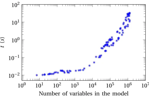
Fig. 8 gives the run times on all standard test cases. Problems were solved on a single core 64 bit Linux machine with 8 GiB RAM, using AMPL 11.0 with CPLEX 12.6 to solve LP problems (only linear cost for generation is considered). The results are for a large number of scenarios for wind power penetration (less than 25%) and demand flexibilities. The number of variables is determined after the pre-solve operation by AMPL which eliminates some of the redundant variables from the model. Fig. 8 shows that the solution times scale well with increasing size of the network.
IV. CONCLUSIONS
In this paper we presented a two stage stochastic pro-gramming approach to solve a multiperiod OPF problem with flexible demands. Demand response is integrated into the model as well to capture demand as a flexible asset. We observed that considerable savings in power generation costs can be made if a small proportion of the demand is flexible. The flexibility of the demand can come from any node of the network provided it respects the network constraints. Numerical results show that the uncertain wind power generation can be optimally utilized using flexibilities from both demand and generation sides. Computational times show the promise of the proposed approach.
100 101 102 103 104 105 106 107 10−2
10−1 100 101 102
Number of variables in the model
t
(
s
[image:8.612.316.558.53.211.2])
Fig. 8. Solution times for solving the proposed model on the IEEE standard test cases. The problems were constructed considering different networks, demand flexibilities and wind penetration levels.
ACKNOWLEDGEMENTS
The authors would like to thank the reviewers for their comments and suggestions. The authors would also like to thankEnerginet.dkfor providing the data that allowed them to generate wind scenarios. The authors are grateful to Aaron Leavy for his help in proofreading the manuscript.
REFERENCES
[1] D. Hawkins, K. Parks, and J. Blatchford, “Improved power system operations with high penetration of wind power: A dialog between academia and industry,” inPower and Energy Society General Meeting, 2010 IEEE, July 2010, pp. 1–4.
[2] N. Hatziargyriou and A. Zervos, “Wind power development in eu-rope,” Proceedings of the IEEE, vol. 89, no. 12, pp. 1765–1782, Dec 2001.
[3] R. Jabr and B. Pal, “Intermittent wind generation in optimal power flow dispatching,”Generation, Transmission Distribution, IET, vol. 3, no. 1, pp. 66–74, January 2009.
[4] J. F. DeCarolis and D. W. Keith, “The costs of wind’s variability: Is there a threshold?” The Electricity Journal, vol. 18, no. 1, pp. 69 – 77, 2005. [Online]. Available: http://www.sciencedirect.com/science/article/pii/S104061900400154X [5] K. Porter and J. Rogers, “Status of centralized wind power forecasting
in north america: May 2009-may 2010,” NREL Subcontract Rep. NREL/SR-550-47853, Tech. Rep., Apr. 2010.
[6] M. Kefayati and R. Baldick, “Harnessing demand flexibility to match renewable production using localized policies,” inCommunication, Control, and Computing (Allerton), 2012 50th Annual Allerton Con-ference on, Oct 2012, pp. 1105–1109.
[7] U. S. Energy Information Adminstration (EIA), “Estimated u.s. residential electricty consumption by end-use,” 2010. [Online]. Available: http://www.eia.gov/tools/faqs/faq.cfm?id=96&t=3 [8] A. Martin and R. Coutts, “Balancing act [demand side flexibility],”
Power Engineer, vol. 20, no. 2, pp. 42–45, April 2006.
[9] A. Conejo, J. Morales, and L. Baringo, “Real-time demand response model,”Smart Grid, IEEE Transactions on, vol. 1, no. 3, pp. 236–242, Dec 2010.
[10] H. Zhong, L. Xie, and Q. Xia, “Coupon incentive-based demand response: Theory and case study,”Power Systems, IEEE Transactions on, vol. 28, no. 2, pp. 1266–1276, May 2013.
[11] Z. Chen, L. Wu, and Y. Fu, “Real-time price-based demand response management for residential appliances via stochastic optimization and robust optimization,”Smart Grid, IEEE Transactions on, vol. 3, no. 4, pp. 1822–1831, Dec 2012.
[12] O. Corradi, H. Ochsenfeld, H. Madsen, and P. Pinson, “Controlling electricity consumption by forecasting its response to varying prices,”
TABLE I
SELECTED RESULTS FROM THE57, 118AND300BUS TEST NETWORKS.
W Wind Penetration (%) D0 D0D(%) D0Flexibility (±%) Improvement (%)
case57
{3} 7.1 {8}{12} 12.030.1 1010 1.654.13 {12} 20.7 {8} 12.0 10 2.00 {9} 9.7 20 3.15
case118
{10} 5.5 {80, 116} 7.4 20 1.97 {54} 2.6 10 0.36 {69, 89} 15.2 {42, 59, 90} 12.6 20 4.25 {54} 2.6 10 0.45
case300
{186, 191} 10.3 {5, 20}{120, 138, 192} 11.04.1 2020 1.133.03 {191, 7003, 7049, 7130} 21.9 {10,44}{120, 138, 192} 1.56.2 1020 0.243.45
[13] Q. Wang, J. Wang, and Y. Guan, “Stochastic unit commitment with uncertain demand response,”Power Systems, IEEE Transactions on, vol. 28, no. 1, pp. 562–563, Feb 2013.
[14] C. Zhao, J. Wang, J.-P. Watson, and Y. Guan, “Multi-stage robust unit commitment considering wind and demand response uncertainties,”
Power Systems, IEEE Transactions on, vol. 28, no. 3, pp. 2708–2717, Aug 2013.
[15] M. Roozbehani, M. Dahleh, and S. Mitter, “Volatility of power grids under real-time pricing,”Power Systems, IEEE Transactions on, vol. 27, no. 4, pp. 1926–1940, Nov 2012.
[16] H. Zhang and P. Li, “Probabilistic analysis for optimal power flow under uncertainty,”Generation, Transmission Distribution, IET, vol. 4, no. 5, pp. 553–561, May 2010.
[17] R. Entriken, A. Tuohy, and D. Brooks, “Stochastic optimal power flow in systems with wind power,” inPower and Energy Society General Meeting, 2011 IEEE, July 2011, pp. 1–5.
[18] C. Saunders, “Point estimate method addressing correlated wind power for probabilistic optimal power flow,” Power Systems, IEEE Transactions on, vol. 29, no. 3, pp. 1045–1054, May 2014.
[19] M. Vrakopoulou, J. Mathieu, and G. Andersson, “Stochastic optimal power flow with uncertain reserves from demand response,” inSystem Sciences (HICSS), 2014 47th Hawaii International Conference on, Jan 2014, pp. 2353–2362.
[20] X. Zhang and G. Hug, “Bidding strategy in energy and spinning reserve markets for aluminum smelters’ demand response,” in Inno-vative Smart Grid Technologies Conference (ISGT), 2015 IEEE Power Energy Society, Feb 2015, pp. 1–5.
[21] D. Phan and S. Ghosh, “Two-stage stochastic optimization for optimal power flow under renewable generation uncertainty,”ACM Trans. Model. Comput. Simul., vol. 24, no. 1, pp. 2:1–2:22, Jan. 2014. [Online]. Available: http://doi.acm.org/10.1145/2553084
[22] A. Papavasiliou and S. S. Oren, “Multiarea stochas-tic unit commitment for high wind penetration in a transmission constrained network,” Operations Research, vol. 61, no. 3, pp. 578–592, 2013. [Online]. Available: http://pubsonline.informs.org/doi/abs/10.1287/opre.2013.1174 [23] C. Murillo-Sanchez, R. Zimmerman, C. Lindsay Anderson, and
R. Thomas, “Secure planning and operations of systems with stochas-tic sources, energy storage, and active demand,”Smart Grid, IEEE Transactions on, vol. 4, no. 4, pp. 2220–2229, Dec 2013.
[24] N. Li, L. Chen, and M. Dahleh, “Demand response using linear supply function bidding,”Smart Grid, IEEE Transactions on, vol. 6, no. 4, pp. 1827–1838, July 2015.
[25] W. A. Bukhsh, C. Zhang, and P. Pinson. Data for stochastic multiperiod opf problems. [Online] Available: https://sites.google.com/site/datasmopf/.
[26] J. R. Birge and F. Louveaux,Introduction to stochastic programming, ser. Springer series in operations research. New York: Springer, 1997. [Online]. Available: http://opac.inria.fr/record=b1093104 [27] J. Zhu,Optimization of Power System Operation. IEEE Press, 2009. [28] P. Pinson, “Wind energy: Forecasting challenges for its operational
management,” Statistical Science, vol. 28, no. 4, pp. 564–585, 11 2013. [Online]. Available: http://dx.doi.org/10.1214/13-STS445 [29] J. M. Morales, A. Conejo, H. Madsen, P. Pinson, and M. Zugno,
Integrating Renewables in Electricity Markets, ser. Springer series in operations research. New York: Springer, 2014.
[30] “IBM ILOG CPLEX Optimizer,” http://www-01.ibm.com/software/integration/optimization/cplex-optimizer/, 2010.
[31] R. Fourer, D. M. Gay, and B. W. Kernighan, AMPL: A Modeling Language for Mathematical Programming. Duxbury Press, Nov. 2002. [Online]. Available: http://www.worldcat.org/isbn/0534388094 [32] R. D. Zimmerman, C. E. Murillo-Sánchez, and R. J. Thomas,
“Mat-power: Steady-state operations, planning, and analysis tools for power systems research and education,” IEEE Transactions on Power Sys-tems, vol. 26, pp. 12–19, 2011.
[33] C. Ferreira, F. Barbosa, and C. Agreira, “Transient stability preventive control of an electric power system using a hybrid method,” inPower System Conference, 2008. MEPCON 2008. 12th International Middle-East, March 2008, pp. 141–145.
[34] Z. Wang and S. Wang, “Grid power peak shaving and valley filling using vehicle-to-grid systems,”Power Delivery, IEEE Transactions on, vol. 28, no. 3, pp. 1822–1829, July 2013.
[35] R. D. Christie. (1999) Power systems test case archive. [Online] Available:http://www.ee.washington.edu/research/pstca/. University of Washington.
Waqquas A. Bukhsh (S’13, M’14) received a B.S. degree in Mathematics from the COMSATS University, Pakistan in 2008 and a Ph.D. degree in Optimization and Operational Research from The University of Edinburgh, UK in 2014.
He is a research associate at the Department of Electronic and Elec-trical Engineering, The University of Strathclyde in Glasgow. His research interests are in large scale optimization methods and their application to the energy systems.
Chunyu Zhang(M’12) received a B.Eng., M.Sc., and Ph.D. degrees from North China Electric Power University, China, in 2004, 2006 and 2014, respectively, all in electrical engineering.
From 2006 to 2012, he joined National Power Planning Center and CLP Group Hong Kong as a senior engineer. He is currently pursuing the Ph.D. degree at the Center for Electric Power and Energy, Technical University of Denmark (DTU), Denmark. His research interests include power systems planning and economics, smart grid and electricity markets.
Pierre Pinson(M’11, SM’13) received a M.Sc. degree in Applied Mathe-matics from the National Institute for Applied Sciences (INSA Toulouse, France) and a Ph.D. degree in Energy from Ecole des Mines de Paris.
![Fig. 1.Flexibility in an aggregated demand. Total demand should beconserved in the time windows [t1,t2] and [t3,t4].](https://thumb-us.123doks.com/thumbv2/123dok_us/1579528.110572/3.612.56.292.48.230/fig-flexibility-aggregated-demand-total-demand-beconserved-windows.webp)