1 INTRODUCTION 1.1 Offshore wind
Reducing the cost of energy is the key for competi-tiveness of offshore wind. A recent study has shown that O&M for a single offshore turbine can cost be-tween £250,000-450,000 per year (GL Garrad Hassan, 2013), which is a significant proportion of the total cost of the project (often up to a third of to-tal cost of energy (Scheu et al. 2012)). In the recent years, a number of tools have been developed in an attempt to reduce the O&M cost of offshore wind. Examples of such tools include OMCE developed by Braam et al. (2011), which estimates annual O&M costs and a tool developed by Dinwoodie et al. (2013), which allows to simulate various operating scenarios, both focused on assessing the benefits of different maintenance solutions.
Furthermore, a comprehensive overview of mod-els applied in wind was provided by Hofmann (2011). The vast majority of offshore wind O&M models are aimed at the pre-operational stages; for example during the planning stage. In the academic domain, very few models, if any, are made for short-to-medium term maintenance decision support. There is a lack of tools which would help operators
decide when and how to maintain offshore wind tur-bines.
There are a number of challenges in maintenance decision making. Firstly, both the short and long-term weather forecasts need to be considered. Ac-cessibility of offshore wind turbines in the North Sea during winter is very low due to stronger winds and high waves; therefore most of the maintenance needs to be carried during the spring to autumn period. Short-term forecasts are used to determine whether the maintenance actions which were planned for the immediate future can be carried out, or will have to be re-scheduled at a later date.
Secondly, assessing the current state of the com-ponent based on condition monitoring data can be difficult. Large volumes of condition monitoring da-ta are analysed by the operators; often cerda-tain alarm trigger values are set. Once the value is exceeded, the operators are warned there may be a problem with the turbine. Trend analysis can be used for fore-casting (García Márquez et al. 2012). Often the me-thods used in the industry are crude, while the solu-tions offered by the academia are overly complicated, discouraging their use in real life (Dujardin et al. 2015).
Thirdly, there are a number of logistical issues to be tackled. Vessels, spares and human resources all
Time Series Semi-Markov Decision Process with Variable Costs for
Maintenance Planning
R. Dawid, D. McMillan & M. Revie
University of Strathclyde, Glasgow
have to be managed efficiently in order to reduce costs. Savings can be found for example through the opportunistic maintenance approach (Ding & Tian, 2011). Furthermore, it may be the case that a wind farm operator has a number of vessels at their dis-posal, each with different properties such as wave height limit, speed or capacity, opening a number of logistical options; selecting the cheapest often won‟t be trivial.
Fourthly, maintenance planners may have to deal with adverse circumstances such as resource short-ages (vessel, spare, human) and unexpected failures. Such events may render previous maintenance sche-dules useless, meaning that the operators need to be able to adapt quickly, while still choosing the cost-optimal actions to take.
Finally, the costs of jack-up vessels can be highly variable, which can also be a factor when planning future maintenance.
In general, maintenance strategies can be time-based or condition-time-based. Researchers proposing time-based strategies (Andrawus et al. 2009), (Kahrobaee & Asgarpoor, 2013) and (Karyotakis & Bucknall, 2010) analyse past failure data to devise optimal maintenance or inspection intervals given costs. However, such strategies lack the flexibility to deal with the majority of issues described above.
Condition-based strategies, such as the one pro-posed by (Byon & Ding, 2010) and (Besnard & Bertling, 2010) are more advanced as the decisions are made based on the condition monitoring data, meaning that maintenance can be performed at a time such that the total cost is minimized. The latter approach is more effective but more difficult to model.
Koopstra & Heijkoop (2015) argue that previous work on models lack an approach that would be in-tegrated (including all the stakeholders‟ require-ments that are necessary to assess the effectiveness of the O&M) and generic (applicable to all wind farms). The condition-based model proposed in this paper attempts to address most of the issues dis-cussed in this section, bridging the gap between the models proposed by the academia and usability on a day-to-day basis during the operation of a wind farm. The rest of this paper is organized as follows: Section 2 describes the methodology used in the model, Section 3 provides a case study to illustrate the model outputs before conclusions are summa-rized in Section 4.
2 METHODOLOGY
The basis of this model is a non-stationary Mar-kov Decision Process (MDP). The use of MarMar-kov models in the wind energy industry has been re-viewed in more detail in (Dawid et al. 2015). MPDs are predominantly used to optimize the offshore
wind turbine maintenance, however, most papers in this field use fixed maintenance intervals, which is more applicable to preventative maintenance rather than corrective. One limitation of the majority of ap-plications of MDPs is that costs are fixed over time (i.e. stationary). In reality, the cost of maintenance in some fields, particularly offshore wind, can be highly variable over time, which has a significant impact on the choice of optimal action. In non-stationary MDPs, the assumption that all the inputs used are fixed over time is relaxed.
A survey for research articles (which included the title, abstract and author keywords) containing the phrase “non stationary Markov decision process maintenance” on the Web of Knowledge website1 re-turned 6 results, suggesting that this approach has not been widely applied in the field of maintenance optimization. Of the 6 papers, only 4 were used for optimizing the maintenance schedule, they are dis-cussed below.
Jin et al. (2016) applied partially observable MDPs, which can deal well with the incomplete in-formation coming from the condition monitoring equipment. The methodology allows both non-stationary transition rates as well as variable costs. Papakonstantinou & Shinozuka (2014) also used partially observable MDPs, however their model on-ly allows non-stationary deterioration and not cost.
Nguyen et al. (2014) employed the MDP metho-dology for maintenance decision making focusing on the effect of technological advancements on the type of decision taken. The model described by Niese & Singer (2013) somewhat resembles the approach proposed here, however, the authors admit that their decision matrix is only marginally useful to the user, partly due to large size; whereas application of a similar method to the problem described in Section 3 of this paper yielded a decision matrix capable of providing useful information to the user, which is perhaps due to the nature of the problem.
The non-stationary approach is well suited to the offshore wind turbine maintenance problem as it al-lows considering both age dependent deterioration and variable costs and rewards as shown in the fol-lowing section.
2.1 Model formulation
The subset of possible actions is denoted as A. Number of states of deterioration is denoted by S. The time horizon for the simulation is denoted by N. A final value F is specified at a time N+1: this represents a reward for the system being in a certain state at the end of the simulation; the better the con-dition of the component at the end, the higher the reward should be (unless the system will be
missioned at the end of the simulation, in which case the rewards for each state should be set to 0).
The transition matrix P, which has a size of SxNxA, comprises of transition rates which can vary over time, making it a Semi-Markov Decision Process (SMDP). The variable failure rates allow the introduction of a bathtub curve, or other failure rate profiles, which is impossible in a standard MDP.
Weather factors are also considered in this model through the use of wind and wave forecasts. Wind prediction is used to estimate the revenue generated - U - by wind turbine on a given day. Significant wave height forecast is used to determine whether the ves-sel will be able to access the wind turbine on a given day. If an action cannot be carried out due to vessel constraints, the logistical cost of carrying an action at that time - L - is set to a high enough number to eliminate the possibility of including this option in the optimal policy. Different actions may require dif-ferent types of vessels; the wave height limit for each vessel can be varied in the model to facilitate this. The costs and rewards of all actions over time are defined in a matrix R which has a size SxNxA. Matrix R is a summation of all costs, both vessel and repair/replacement cost, as shown in Equation 1.
Costs of actions C and logistical costs L are de-pendent on time and the type of action taken, while rewards U are dependent on the wind forecast (time dependent) and the state of the wind turbine; a failed turbine will produce no revenue. In case of compo-nents such as blades, the age may also have a signif-icant effect on how much power is produced; per-formance of deteriorated blades was shown to be significantly lower compared to brand new ones (Gaudern, 2014) – this can be easily implemented in the model.
2.2 Model implementation
One of the procedures for solving MDPs is through value iteration using Bellman equation (Bellman, 1957). After an initial guess of the value is made, the iterations are repeated until convergence, upon which the value of being in a certain state is known. The Bellman‟s equation used in the model proposed in this paper, is as follows:
where V is the value matrix and d is the discount factor. Here, the iterations are in fact time steps, the simulation starts at t=N and is carried out “back-wards”. The final value of the asset F becomes the V(st+1) in the first iteration, allowing to calculate the
values for each state at time t=N-1. The following iteration is no longer based on F, but on the value
[image:3.595.312.563.248.471.2]calculated in the previous iteration. As it is assumed that the final value of each state specified by the user is exact, the iterative process to find the converged value of a state used in standard MDP solutions is no longer required. In practice, such assumption is not unreasonable, as the final value of an asset at the end of the simulation would be approximately known by the wind farm operator – the value of a turbine being either in an operational or failed state can be quanti-fied through economic analysis. The iterative process ends when t=1. The resulting matrix V will be of size SxAxN. Optimal actions yielding maxi-mum value are selected based on matrix V. This will result in an optimal policy of a size SxN, which re-commends an action for each state, at each time. The outline of the model is shown in Figure 1.
Figure 1. The outline of the model.
3 CASE STUDY
3.1 Model inputs and assumptions
The methodology described in the previous sec-tion was applied to a simple case study based on fic-tional data. The actions available to the user are to replace, repair and do nothing. Imperfect repairs were used in this case study, meaning that there is a 90% chance that the component‟s state will improve by one after repair, 10% chance it will stay the same. Repair has no effect if the turbine is in a “failed” state. Replacement will always bring the state of the component to brand new condition.
of deteriorating from “bad” to “failed”. The “accele-rating” failure rate reflects the fact that often by the time a problem is detected through condition moni-toring data analysis the time to failure is relatively short.
The costs of repairing and replacing the compo-nent were defined, as shown in Table 1.
Table 1. Cost of actions given state (spares/materials).
_____________________________________________
Action cost (£„000) Do nothing Repair Replace _____________________________________________
Brand new 0 5 30
Good 0 5 30
Bad 0 5 30
Failed 0 30 30
[image:4.595.303.558.238.295.2]_____________________________________________ In addition to the cost of repair itself, the cost of vessel hire can also be significant, particularly when considering the jack-up vessels. In this case study, it is assumed that repairs will be carried out by a Crew Transfer Vessel (CTV), while replacements will re-quire a jack-up vessel. Wind farm operators usually do not own jack-up vessels – they have to be hired from an external company. Often the jack up vessels have to be booked well in advance; short term hires can be very expensive, which was reflected in the inputs to this model, as shown in Table 2. Table 2. Cost of vessel hire over time. _____________________________________________ Logistics cost (£„000) CTV/Repair Jack-up/Replace _____________________________________________ Days 1-2 10 350
Days 3-9 10 150
Days 10-12 10 100
Days 13-15 10 80 _____________________________________________
It was assumed that the significant wave height limit below which the vessel can operate is 1.5m for CTVs and 2m for jack-up vessels. If the either of the vessels limits is exceeded, the cost of action is set to £1,000,000, effectively eliminating the possibility of it being selected in the optimal policy.
For simplicity, it is assumed that the wind speed is linearly correlated to wave height, with maximum generated revenue (equal to £10,000/day) at wave height equal to 2 meters. The amount generated at other wave heights can be calculated using Equation 3:
where R2m is the revenue generated by a turbine
when the wave height is 2 meters, h is the wave height. It was assumed that if a repair is carried out, the turbine will only be able to generate 85% of the revenue it would have generated on that day, if it had not been shut down for repairs. If the state of the wind turbine was “failed”, or if the turbine was un-dergoing a replacement, the revenue generated that
day would be £0. It was assumed that the wind tur-bine will produce the same amount of revenue, whether the state of the component is “brand new”, “good” or “bad”.
Time units were set to be days. Discount factor was defined as 0.999 (per unit time, i.e. day). The fi-nal rewards at the end of the simulation were set to £150,000, £140,000, £50,000 and £0 for states “brand new”, “good”, “bad” and “failed” respective-ly.
[image:4.595.308.566.420.501.2]A summary of wave height forecast and vessel availability is shown in Figure 2. It allows the opera-tor to see at a glance, on what days the repairs and replacements will not be possible due to wave height constraints.
Figure 2. Wave height forecast and predicted vessel availa-bility.
3.2 Results
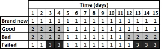
The main output of the model is a set of optimal actions for each time step, for each state of the sys-tem, as shown in Figure 3.
Figure 3. Optimal actions for each state at each time. Action 1 is “do nothing”, 2 is “repair”, 3 is “replace”.
From the optimal policy shown in Figure 3, it can be seen that whenever the system is in the state “brand new” nothing should be done and whenever the system is in a “bad” state, a repair should be car-ried out (weather permitting).
Optimal actions for states good and failed are more interesting; they are highly dependent on the time due to the variable rewards and costs.
[image:4.595.33.268.420.487.2]Fig-ure 2). Repairing in day 1 then makes sense, as the lost revenue due to carrying out a repair would be minimized.
Effectively, the optimal policy‟s recommendation is to attempt to get the system in the “brand new” state before wave height reaches 1.5m, as once it does, the cheap option of repair will not be available to the operator for the next week. Once the repair ac-tion becomes possible again on day 12, it is no long-er essential to be in the “brand new” state, so repairs are only carried out when the system is in a “bad” state, in order to avoid failure, which is expensive.
Looking at the fourth row of Figure 3, the optimal action in a failed state in days 1-2 is to do nothing, which is due to the very high cost of jack-up vessel hire. On day 3, when the cost lowers significantly, it is optimal to replace, however, only until day 4. From then on, it makes more sense to wait to replace until day 13 as this is when the logistical cost is at its lowest. This could be explained by the fact that the difference in logistical cost on days 5 and 13 is more than the revenue the turbine would have generated during the time between days 5-12 (although this is not strictly true, as there is a possibility, albeit small, that despite being repaired on day 5, the turbine would fail again before day 12, which is also consi-dered in this methodology through the use of Bell-man equation).
3.3 Potential model uses
This model was designed with practical applica-tion in mind. It takes seconds to run, is defined by a handful of equations, making it easy for the practi-tioners to use and understand. There is no constraint on what component the model could be applied to; in fact it would be possible to use the condition monitoring data to classify the condition of the whole turbine, eliminating the need for multiple models.
The model would work well in conjunction with a tool for condition monitoring data analysis, capable of classifying the current condition of the compo-nent. One of the possible uses of this methodology could be to forecast future demand for jack-up ves-sels or CTVs, depending on the predicted future condition of the component, the weather and ex-pected costs of repair. It is possible that further cost savings could be obtained by applying the model to spares management and human resource manage-ment.
Suppose the condition monitoring data suggests that a failure, which requires a jack up vessel, will occur in a week‟s time (day 7 in Figure 3). An in-stinctive action would be to request a jack-up vessel for day 7 immediately, to avoid further price in-crease. The resulting cost would be £150,000 and the income generated by the turbine until the end of the
time horizon in this simulation given the expected wind speed would be £63,000 (days 8-15, assuming the state remains “brand new”). Instead, if the op-timal policy shown in Figure 3 is followed, the cost of jack-up hire will be £80,000 and the revenue gen-erated £11,500. Hence the total cost of the first op-tion is £87,000 compared to £68,500 for the optimal policy, resulting in a significant cost saving of £18,500.
As the model‟s accuracy is highly dependent on the weather forecast, it would be advisable to run it on a daily basis to ensure the most accurate inputs are used. For example, using the policy from Figure 3, if the condition of the turbine is classified as bad on day 1, the operator knows that if a jack-up vessel will be required in the next 10 days, it would be most cost-effective to hire it for days 3 and 4.
The case study described in Section 3.1 is a sim-ple one, designed to be easily interpreted. In reality, more states, repair actions and vessel options can easily be considered by the model, allowing it to not only inform the operator when, but also how to maintain the wind turbine.
4 CONCLUSIONS
The model presented in this paper has the poten-tial to reduce the cost of offshore wind O&M by providing decision support to wind farm operators. Resulting policy is optimal as minimizes the total cost, taking into account the vessel constraints, both logistical and repair costs, the lost revenue, current condition of the turbine and forecasted weather con-ditions.
The novelty of the approach described here is the inclusion of time varying costs and failure rates, which transforms the widely used and relatively simple MDP framework into a useful tool for main-tenance decision support.
The model can be used for both short and me-dium term maintenance planning; it is highly flexible as factors such as time horizon, vessels and their costs and failure rates can be changed easily. As the model is relatively simple and not computationally intensive; it will likely appeal to practitioners.
5 REFERENCES
Andrawus, J. a., Watson, J., & Kishk, M. (2009). Wind Turbine
Maintenance Optimisation: principles of quantitative maintenance optimisation. Wind Engineering, 31(0044), 101–110. doi:10.1260/030952407781494467
Bellman, R. (1957). Dynamic Programming. Princeton University Press.
Condition-Based Maintenance Optimization Applied to Wind Turbine Blades. IEEE Transactions on Sustainable Energy, 1(2), 77–83. doi:10.1109/TSTE.2010.2049452
Braam, H., Obdam, T., van de Pieterman, R., & Rademakers, L. (2011). Properties of the O&M Cost Estimator (OMCE), (July), 154. Retrieved from
http://www.ato.nl/db/WAS4e3a7e8d3ae78/Properties_of _the_O_M_Cost_Estimator_July_2011.pdf
Byon, E., & Ding, Y. (2010). Season-Dependent Condition-Based Maintenance for a Wind Turbine Using a Partially Observed Markov Decision Process. IEEE Transactions
on Power Systems, 25(4), 1823–1834.
doi:10.1109/TPWRS.2010.2043269
Dawid, R., Mcmillan, D., & Revie, M. (2015). Review of Markov Models for Maintenance Optimization in the
Context of Offshore Wind, 1–11.
Ding, F., & Tian, Z. (2011). Opportunistic Maintenance
Optimization for Wind Turbine Systems Considering Imperfect Maintenance Actions. International Journal of Reliability, Quality and Safety Engineering, 18(05), 463– 481. doi:10.1142/S0218539311004196
Dinwoodie, I., McMillan, D., Revie, M., Lazakis, I., & Dalgic, Y. (2013). Development of a combined operational and
strategic decision support model for offshore wind.
Energy Procedia, 35, 157–166.
doi:10.1016/j.egypro.2013.07.169
Dujardin, Y., Dietterich, T., & Chad, I. (2015). α -min : A Compact Approximate Solver For Finite-Horizon POMDPs, (Ijcai), 2582–2588.
García Márquez, F. P., Tobias, A. M., Pinar Pérez, J. M., & Papaelias, M. (2012). Condition monitoring of wind turbines: Techniques and methods. Renewable Energy,
46, 169–178. doi:10.1016/j.renene.2012.03.003
Gaudern, N. (2014). A practical study of the aerodynamic
impact of wind turbine blade leading edge erosion.
Journal of Physics: Conference Series, 524, 012031. doi:10.1088/1742-6596/524/1/012031
GL Garrad Hassan. (2013). A Guide to UK Offshore Wind Operations and Maintenance. Scottish Enterprise and The Crown Estate.
Hofmann, M. (2011). A Review of Decision Support Models for Offshore Wind Farms with an Emphasis on Operation and Maintenance Strategies. Wind Engineering, 35, 1–16.
doi:10.1260/0309-524X.35.1.1
Jin, L., Bayarsaikhan, U., & Suzuki, K. (2016). Optimal control
limit policy for age-dependent deteriorating systems under incomplete observations. Proceedings of the Institution of Mechanical Engineers, Part O: Journal of
Risk and Reliability, 230(1), 34–43.
doi:10.1177/1748006X15589208
Kahrobaee, S., & Asgarpoor, S. (2013). A hybrid
analytical-simulation approach for maintenance optimization of deteriorating equipment: Case study of wind turbines.
Electric Power Systems Research, 104, 80–86. doi:10.1016/j.epsr.2013.06.012
Karyotakis, A., & Bucknall, R. (2010). Planned intervention as a maintenance and repair strategy for offshore wind
turbines. Proceedings of the Institute of Marine Engineering, Science and Technology Part A: Journal of Marine Engineering and Technology, 27–35.
Koopstra, H., & Heijkoop, G. (2015). Integrated Decision Support Tool for Planning and Design of Offshore Wind O & M Strategies. EWEA, 1–5.
Nguyen, T. P. K., Castanier, B., & Yeung, T. G. (2014). Maintaining a system subject to uncertain technological evolution. Reliability Engineering and System Safety,
128, 56–65. doi:10.1016/j.ress.2014.04.004
Niese, N. D., & Singer, D. J. (2013). Strategic life cycle
decision-making for the management of complex Systems subject to uncertain environmental policy. Ocean
Engineering, 72, 365–374.
doi:10.1016/j.oceaneng.2013.07.020
Papakonstantinou, K. G., & Shinozuka, M. (2014). Optimum inspection and maintenance policies for corroded structures using partially observable Markov decision
Processes and stochastic, physically based models.
Probabilistic Engineering Mechanics, 37, 93–108. doi:10.1016/j.probengmech.2014.06.002
Scheu, M., Matha, D., Hofmann, M., & Muskulus, M. (2012). Maintenance strategies for large offshore wind farms.
Energy Procedia, 24(January), 281–288.