Optimisation of maintenance policy under
parameter uncertainty using portfolio theory
Shaomin Wu
1Kent Business School, University of Kent, Canterbury, Kent CT2 7PE, UK
Frank P.A. Coolen
Department of Mathematical Sciences, Durham University,
Durham DH1 3LE, UK
Bin Liu
Department of Systems Engineering and Engineering Management,
City University of Hong Kong, Hong Kong, China
Abstract
In reliability mathematics, optimisation of maintenance policy is derived based on
reliability indexes such as the reliability or its derivatives (e.g., the cumulative
fail-ure intensity or the renewal function) and the associated cost information. The
reliability indexes, also referred to as modelsin this paper, are normally estimated
based on either failure data collected from the field or lab data. The uncertainty
associated with them is sensitive to factors such as the sparsity of data. For a
com-pany that maintains a number of different systems, developing maintenance policies
for each individual system separately and then allocating maintenance budget may
not lead to optimal management of the model uncertainty and may lead to
cost-ineffective decisions. To overcome this limitation, this paper uses the concept of risk
aggregation. It integrates the uncertainty of model parameters in optimisation of
maintenance policies and then collectively optimises maintenance policies for a set
of different systems, using methods from portfolio theory. Numerical examples are
Key words: Maintenance, parameter uncertainty, portfolio theory, maintenance
policy
1 Introduction
Optimisation of maintenance policies, in particular planning preventive maintenance
activ-ities, is an important research topic in reliability mathematics with great relevance to real
world applications. It helps the asset managers to monitor the condition of assets and to
un-derstand the financial exposure associated with maintenance costs. Many existing methods
for maintenance policy optimisation are based on the assumption that the true and precise reliability indexes, also referred to asmodelsin this paper, of asset reliability can be obtained.
This assumption is unrealistic, in the sense that model uncertainty exists, in particular if
model parameters are estimated based on available data. Existing methods for maintenance
planning tend to neglect such model uncertainty, which may be particularly problematic if
many similar units need to be maintained.
This paper considers maintenance planning under uncertainty about parameter values in an assumed model. The approach proposed is based on the use of sample data to estimate
the optimal maintenance policy, which minimizes the expected cost and its variance. The
method involves defining a model and estimating its parameters from data. Consequently,
estimating the variance for the expected cost (which is a function of the parameters) involves
the variance estimated for these parameters.
1.1 Prior work
Maintenance policies are normally developed through applying the least-cost methodology, in
which the optimum maintenance policy with the minimised expected cost rate on maintaining
a stand-alone system within a given time period is sought (Wang, 2002). To formulate the
expected cost rate requires reliability indexes such as the cumulative failure function and the
renewal indexes, and cost information such as cost of failure and cost of maintenance (see
Moghaddass et al. (2015); Zhang & Yang (2015), for example).
Reliability indexes are normally estimated based on lab data and failure data collected from
the field (Wu & Scarf, 2015). The sparsity of such data varies from case to case, which
can result in different efficiency levels of the maintenance models, or model uncertainty.
It is known that three main sources of uncertainties in models stem from (1) data
uncer-tainty (e.g. measurement errors, small sample size, etc); (2) model parameters (unceruncer-tainty
of model parameters); and (3) model structural uncertainty (models are too simple or too
complicated). As identified by Aven (2001), the following two levels of uncertainty exist
regarding maintenance models.
Level 1. At the first level, there is uncertainty about observable quantities such as the time
to the next failure, for which we develop probability models to describe the uncertainty.
Level 2. At the second level there is uncertainty regarding unobservable quantities such as
model structure and model parameters, which stems from the quality of the first level such
as the size of observed failure data.
As highlighted by Percy et al. (2010), failure data can be sparse and maintenance
schedul-ing problems are notoriously sensitive to the inaccuracy inherent in model structure and
parameter estimates.
In reality, there may be the following scenarios with regard to data collection.
No data scenario. For newly developed or highly reliable equipment, there may be no
failure data that can be collected. In this scenario, the technique of expert elicitation can
be pursued to estimate the reliability of such equipment. Apparently, uncertainty exists in
the probability distributions estimated by the experts. It should be noted that “elicitation
of probability distributions is a far from perfect process” (O’Hagan & Oakley, 2004) and
“overconfidence is one of the most common (and potentially severe) problems in expert
judgement ”(Lin & Bier, 2008).
Sparse data scenario. When the number of observations collected is small, huge uncertainty
may exist in the estimated parameters of an assumed probability distribution. In the literature, two main approaches have been developed to tackle this problem. They are the
re-sampling technique and the Bayesian updating approach. For example, Laggoune et al.
considering the problem of the small size of failure data samples. Their work leads to a more
general result, as it considers the parameter distribution, according to the available number
of failure data. Fang & Huang (2008) uses the Bayesian updating approach to tackling the
scenario where data are sparse. Their work, nevertheless, investigates approaches to dealing
with model uncertainty for a specific maintenance policy of a given product (system) and may therefore not be ideal for a maintenance planner looking after a set of different types
of assets, as argued in the following.
Of course, there is also the scenario of large amounts of data, leading to the possible use of
‘big data’ methods. This is not addressed in this paper because the typical issues of model
uncertainties are very different in this case. Recently, de Jonge et al. (2015) studied the
effect of parameter uncertainty on the optimum age-based maintenance strategy. The effect of uncertainty is evaluated by considering both a theoretical uniform lifetime distribution
and a more realistic Weibull lifetime distribution.
In the reliability literature, despite presence of uncertainty in maintenance models,
main-tenance policies are developed to a large degree of mathematical elegance, or “ad hoc”,
meaning that new maintenance models2 have been designed in an attempt to represent
particular preferences and that little consideration has been paid to the presence of model
uncertainty caused by sparsity of data. As a result, most maintenance models and policies,
while possessing certain attractive mathematical properties, have been lacking applicability
and relevance in the real world.
1.2 Our approach
Since maintenance models possess different levels of uncertainty, it may be cost-ineffective
if a company, which maintains a set of different systems, ignores the uncertainty, develops
maintenance policy for each individual system separately, and then allocates maintenance
budget to each system respectively. A more cost-effective approach may be to collectively
optimise maintenance policies for the set of systems, with consideration of model uncertainty.
This motivates the research presented in this paper.
2 In this paper, maintenance policy means the frequency of maintenance activities that are
This paper proposes to use portfolio theory, which is widely used in the finance sector
(Krokhmal et al., 2011) for managing risk and uncertainty, to collectively optimise
nance policies for a set of systems. It will concentrate on parameter uncertainty of
mainte-nance models. This uncertainty will be summarised by the variance of the estimated
param-eters.
The proposed approach can be interesting to both practitioners and researchers. It is
use-ful to the firms that maintain different types of systems but the sparsity of the historical
reliability data (e.g., time between failures, or maintenance performance) of different
sys-tems may vary, and it can also be applied to optimise a collection of different policies of
preventive and predictive maintenance activities. Here, firms can be maintenance companies or manufacturers. For example, a maintenance firm may need to allocate its limited budget
on maintenance, or a manufacturer may want to decide the length of the extended warranty
for a set of different products sold. In the meantime, academic researchers may be interested
to extend this work, for example, some further research topics are listed in the conclusion
section of this paper.
To our best knowledge, this is the first paper attempting to collectively optimise different
types of maintenance policies (for example, block replacement, age replacement policies, and
failure limit policies can be optimised simultaneously) for different systems. The optimization
of the maintenance policy through the minimization of the expected cost and its variance is
the big novel of the present paper.
1.3 Overview
It should be noted that, in this paper, the term risk refers to the financial risk caused by
model uncertainty. In reliability mathematics, there are many publications discussing
risk-based maintenance (Zhu & Frangopol, 2013; Hu & Zhang, 2014), in which risk, such as
risk of health damage or property loss, is caused by system failures. Further, in this paper
the term uncertainty refers to the “aleatory uncertainty” (or uncertainty due to variability)
which represents randomness of samples.
The remainder of this paper is structured as follows. Section 2 formulates the problems
4 discusses the proposed techniques. Section 5 gives numerical examples on optimisation of
maintenance policy. Some concluding remarks are presented in Section 6.
2 Uncertainty of the expected cost
In this section, parameter uncertainty of three maintenance models and their implications
are discussed.
2.1 Three replacement policies
In the following, we use three basic replacement policies as examples. Time required for repair
or replacement is assumed to be negligible. Of course, the optimisation method proposed
in this paper can also be applied to a combination of preventive policies and predictive
maintenance policies.
Denote F(t|θ) as the lifetime distribution function, ¯F(t|θ) = 1 − F(t|θ), and θ as the
parameter vector of F(t|θ) (for example, θ in the Weibull distribution includes both the
shape parameter and the location parameter). LetM(t|θ) =P∞
n=1F(n)(t|θ), whereF(n)(t|θ)
is the nth Stieltjes convolution ofF(t|θ) and F(n)(t|θ) =Rt 0F(n
−1)(t−u|θ)dF(u|θ).
We consider the following three maintenance policies, with the optimality criteria all based on the renewal reward theory (Barlow & Proschan, 1965). One could also include different
criteria (Coolen-Schrijner & Coolen, 2006), this is left as a topic for future research.
Age replacement Under this policy, one replaces a unit with a new identical unit either at
a pre-determined ageT or upon failure if it occurs earlier. Letc1 be the cost of replacement
for a failed unit and c2 be the cost of scheduled replacement. Then according to Barlow
& Proschan (1965), the expected cost is given by
Ca(T|θ) =
c1F(T|θ) +c2F¯(T|θ) RT
0 F¯(t|θ)dt
. (1)
Block replacement Under this policy, a unit is replaced with a new identical unit upon
failure or at fixed times kT(k = 1,2, ...,). Let c1 be the cost of replacement for a failed
(1965), the expected cost is given by
Cb(T|θ) =
c1M(T|θ) +c2
T . (2)
Periodic replacement with minimal repair Under this policy, a unit is replaced at fixed
timeskT(k= 1,2, ...) with a new identical unit. If a unit fails between replacements, min-imal repair is made to restore the unit back to work. Denote c1 as the cost of minimal
repair and c2 as the cost of scheduled replacement. Then according to Barlow & Proschan
(1965), the total expected cost is given by
Cp(T|θ) =
c1Λ(T|θ) +c2
T , (3)
where Λ(x|θ) is the cumulative intensity function of the repairable unit.
Note that it is reasonable to assume that c1 > c2. This assumption will be followed in this
paper.
2.2 Uncertainty of the expected cost
As discussed in Section 1.1, the uncertainty of a model is larger (smaller) if the model is
developed based on a smaller (larger) sample size. That is, for example, in the equations (1),
(2), and (3), the variances of estimated parameters θ are larger for small sample size than
those for large sample size. Now the following two questions are important.
Q1. how to estimate the variance for parameters θ; and
Q2. how to estimate the variance for a function of parametersθ.
Different methods for Q1 can be found in the literature. For example, in case of fitting the
Weibull distribution, one may have three scenarios: (1) when there is no data available or a
very small sample size (n <10 for example) for developing a model, expert elicitation (EE) or EE with Bayesian updating may be pursued to estimate the variance (Speirs-Bridge et al.,
2010); (2) when the sample size n is between 10 and 52, the weighted least-square method is preferable (Wu et al., 2006); and (3) If one has a larger sample size (n ≥ 53), then the maximum likelihood may be used (Wu et al., 2006).
Cb(T|θ), and Cp(T|θ) after the variance of θ is given. That is, one needs to estimate the
variance for g(θ) if the variances forθ is given, hereg(θ) =Ca(T|θ) for the age replacement
policy, for example.
In the literature, there are some approaches to estimating confidence intervals for functions
of parameters, for example, the bootstrap method Krinsky & Robb (1986) and the δmethod (see p. 172, Weisberg (2014)).
2.3 Decision problem
Suppose a company is maintaining n different systems and attempting to develop mainte-nance policies for those systems. Denote Ci(Ti|θi) as the expected cost of the maintenance
policy for system i (i = 1,2, ..., n), where Ti is the vector of decision variables such as
pre-ventive maintenance intervals for maintaining system i, and θi includes the parameters in
the reliability index of system i.
Then, the expected total cost of maintenance of the n systems is given by
C(T|θ) =
n
X
i=1
Ci(Ti|θi), (4)
where θ = (θ1, . . . ,θn) and T = (T1, . . . , Tn).
In the literature, the existing approach to optimising maintenance policy is to minimise
eachCi(Ti;θi), respectively, and then to allocate the total amount to each of then systems.
However, as θi is estimated based on observations, its efficiency can vary with sample sizes.
In other words, θi can be treated as a random variable. Consequently, the total amount,
C(T|θ), becomes a random variable. This leads to different attitudes of the decision makers
in order to deal with the possible variation in expected costs resulting from uncertainty
about the parameter value. For example, assume that a company is maintaining a number
of systems. Suppose that there are several options of maintenance policies are designed and
they have different total expected cost C(T|θ) and different variance Vθ(C(T|θ)). Then, the
selection of options may depend on the company’s risk attitude as well as its budget. (1) If the company is risk-averse, it may choose an option with lower risk (i.e., Vθ(C(T|θ)));
(2) if the company is risk-prone, it may choose an option having lower expected cost (i.e.,
That is, to choose an option depends not only on the total expected cost C(T|θ), but also
on the variance Vθ(C(T|θ)). Of course, the total attitude towards risk can be taken into
account, for example through the use of utility functions. However, this is often difficult
to measure meaningfully, in portfolio theory the variance is typically used as a surrogate
measure for risk. In other words, company’s risk attitude plays an important role in decision making. Risk-averse planners differ from risk-loving planners in that they are concerned more
about the decisions that minimise risk than about those that minimise the expected cost.
In summary, factors influencing decision making include the total expected cost, decision
maker’s risk attitude, and available budget. Those factors will be considered when we
opti-mise maintenance policies in the following sections.
3 Collective optimisation of risk
In this section, we propose three new methods to optimise maintenance policies.
3.1 Methods of collectively optimising PM policies
To incorporate risk in optimisation of maintenance policies, one may choose one of the
following three optimisation problems.
Option 1. One may explicitly trade risk against the expected cost in the objective function:
min T∈R C(
T|θ) +ρVθ(C(T|θ)). (5)
where ρ is a pspecified non-negative parameter and it is typically assumed to be re-stricted to values in [0,1]. The value of ρ reflects the decision maker’s risk attitude. For example, if the decision maker is risk averse, ρ may be set larger. In the current formu-lation ρ would not be unit-less, its unit would be the chosen monetary unit to the power
−1. Note that alternative formulations replace the variance by the standard deviation, or divide both the expected costs and the variance by similar functions, for example cor-responding to a standard scenario, in order to do away with units and hence to make
the sum meaningful. In all cases though, this option relates to an explicit weighting of
as only allowing solutions on a Pareto boundary, that is any decrease in expected costs at
an optimal value will lead to increase of the risk.
Option 2. One may select the decision T that minimises the expected cost C(T|θ) while
imposing a maximum level of risk Vθ(.):
min T∈RC(
T|θ), (6)
subject to : Vθ(C(T|θ))≤ν0.
where ν0 reflects decision maker’s risk attitude. For example, if the decision maker is risk
averse, ν0 may be set small.
Option 3. A third alternative can be to minimise the risk Vθ(.) while imposing a maximum level of the expected cost C(T|θ):
min
T∈R Vθ(C(
T|θ)), (7)
subject to : C(T|θ)≤C0.
where C0 reflects the budget constraint.
Option 3 is mainly used for portfolio management in finance. However, it is thought that
its inclusion is relevant as practical maintenance planning under quite severe budget
limita-tions is very common, with maintenance managers often explicitly working towards using an
allocated budget while aiming to keep variance low, a reflection of low risk of huge overspend.
In the following, we use letters a, b and p in the subscripts of relevant quantities to distin-guish notation of the age replacement policy, the block replacement policy and the periodic
replacement with minimal repair policy, respectively.
Suppose a set of one-unit systems composed ofmasystems maintained with age replacement
policy, mb systems maintained with block replacement policy, and mp systems maintained
with periodic replacement with minimal repair policy. We assume throughout that all ma
systems subject to age replacement are exchangeable with regard to their time to failure and
costs associated with running and maintaining them. Of course, in practice this may not be entirely realistic. The method presented in this paper can be quite easily adapted to more
complicated scenarios, studying such scenarios from practical perspective is an important
We now have the following three properties.
In the following, we assume that the parameters in maintenance policies for different systems
are statistically independent.
Property 1 With the optimisation Option 1, the objective function is given by
G(T) =maCa(Ta|θa) +mbCb(Tb|θb) +mpCp(Tp|θp)+
ρm2aVθ(Ca(Ta|θa)) +m2bVθ(Cb(Tb|θb)) +m2pVθ(Cp(Tp|θp))
. (8)
Assume fa(Ta|θa)/F¯a(Ta|θa) is continuous and increasing with respect to Ta. Then there
exists an optimum solution T∗
= (T∗
a, T
∗
b, T
∗
p) that minimises the following problem:
min T∈RG(
T). (9)
The proof of the properties can be found in the Appendix. We should emphasize here that the
variance of the expected costs is due to the assumed uncertainty in the parameter value. At
planning stage, the expected costs for all systems that are maintained with age replacement
are the same, and hence all these systems will be maintained with the use of the same optimal
value for Ta. Hence, when we take the variance of the sum of these ma expected costs, we
get the term m2
a times the variance expression as given above.
Property 2 With the optimisation Option 2, the objective function is given by
min
T∈R maCa(Ta|
θa) +mbCb(Tb|θb) +mpCp(Tp|θp), (10)
subject to :m2aVθ(Ca(Ta|θa)) +m2bVθ(Cb(Tb|θb)) +m2pVθ(Cp(Tp|θp))≤ν0. (11)
Then, one can use the following algorithm to find the optimum PM policies.
Algorithm 2. The optimisation process under Option 2 can be done with the following
procedures.
Step 1. Find the maintenance policy for each system respectively, and then check if the
Step 2. Solve equations (12–15) to obtain optimum solutions.
∂Ca(Ta|θa)
∂Ta
+µma
∂Vθ(Ca(Ta|θa))
∂Ta
= 0, (12)
∂Cb(Tb|θb)
∂Tb
+µmb
∂Vθ(Ca(Tb|θb))
∂Tb
= 0, (13)
∂Cp(Tp|θp)
∂Tp
+µmp
∂Vθ(Cp(Tp|θp))
∂Tp
= 0, (14)
µ(m2aVθ(Ca(Ta|θa)) +m2bVθ(Cb(Tb|θb)) +m2pVθ(Cp(Tp|θp))−ν0) = 0, (15) where µ is a Lagrange multiplier.
Property 3 With the optimisation Option 3, the objective function is given by
min T∈R m
2
aVθ(Ca(Ta|θa)) +m2bVθ(Cb(Tb|θb)) +m2pVθ(Cp(Tp|θp)), (16) subject to :maCa(Ta|θa) +mbCb(Tb|θb) +mpCp(Tp|θp)≤C0. (17)
Then, one can use the following algorithm to find the optimum PM policies.
Algorithm 3. The optimisation process under Option 3 can be done with the following
procedures.
Step 1. If C0 is large enough, the optimum maintenance policy is that no replacement should
not be conducted; otherwise, go to step 2;
Step 2. One can solve equations (18–21) to obtain optimum solutions.
µ∂Ca(Ta|θa) ∂Ta
+ma
∂Vθ(Ca(Ta|θa))
∂Ta
= 0 (18)
µ∂Cb(Tb|θb) ∂Tb
+mb
∂Vθ(Ca(Tb|θb))
∂Tb
= 0 (19)
µ∂Cp(Tp|θp) ∂Tp
+mp
∂Vθ(Cp(Tp|θp))
∂Tp
= 0 (20)
µ(maCa(Ta|θa) +mbCb(Tb|θb) +mpCp(Tp|θp)−C0) = 0 (21)
where µ is a Lagrange multiplier.
The equations in Step 2 in both Algorithm 2 and Algorithm 3 follow from the well-known
Karush-Kuhn-Tucker first-order necessary condition for a candidate solution point to be an optimum solution. Those conditions are not sufficient. To seek the sufficient conditions, or
the second order sufficient conditions, the reader is referred to Theorem 4.46 in page 99 in
3.2 Special cases
To apply the above-proposed methods in optimisation problems shown in Eqs (5)–(7), one
needs to calculate Vθ(Ca(Ta|θa)), Vθ(Cb(Tb|θb)) and Vθ(Cp(Tp|θp)). Below we give some example methods of calculating those quantities for the case when the lifetime distribution
is the Weibull distribution.
Calculation of Vθ(Ca(Ta|θa)).
Given lifetime distributionF(t|θ) = 1−exp
−tβ−
1
a αa
. Assume ma units are under a Type
I censoring scheme: unit i may fail atXi before the threshold time τa or survive over the
time interval (0, τa). From Sirvanci & Yang (1984), the estimator of αa and its variance
are given by
ˆ
αa= ma
X
i=1
Vβa−1 i
M , (22)
and
V( ˆαa) =
α2 a p + α2 a β2 a
(1 +I1p+ logαa)2V(βa), (23)
respectively, where Vi = min{Xi, τa}, M is the number of failures occurring in [0, τa], p
can be estimated by ˆp= maM ,I1p = 1pR0plog log1−1tdt, and h(p) = log log
1
1−p −I1p.
The estimator of βa and its variance are given by
ˆ
βa= ma
X
i=1
(logτa−logXi)Ii
M h(p) , (24)
and
V( ˆβa) =
β2
aI2p−βa2pI12p+βa2p3(1−p)
h
(1−p) log 1 1−p
i−1
− h(pp)
2
(ph(p))2 , (25)
respectively, where Ii is the indicator of the event [Xi < τa]. That is, Ii = 1 if item i fails
in [0, τa] and Ii = 0 otherwise, andI2p =R0p
log log11−t2dt. The covariance of ˆβa and ˆαa is given by
cov( ˆαa,βˆa) =
1
β2
a
[−αaβa(1 +I1p+ logαa)V(βa)]. (26)
One may use the δ method to calculate the variance of the expected cost for the age replacement policy.
Calculation of Vθ(Cb(Tb|θb)).
Given lifetime distributionF(t|θ) = 1−exp
−
tβ−
1
b αb
, in order to calculate the variance
are under a Type I censoring scheme: unit i may fail at Xi before the threshold time τb
or survive over the time interval (0, τb). Jiang (2010) develops the following formula to
approximateM(t|θ),
M(t|θ) = q
1−exp
−
tβ−1
b αb
+ (1−q)
tβ−1
b
αb
, (27)
where q = 1−exp
− 1
0.8818 1−βb
βb
0.9269
. Based on the above approximation of M(t) and similar estimators as those shown in Eqs. (22)—(25)3, one can use the δ method to
calculate the variance of Vθ(Cb(Tb|θb)) for the block replacement policy.
Calculation of Vθ(Cp(Tp|θp)).
Calculating Vθp(Cp(Tp|θp)) differs from calculating Vθa(Cp(Ta|θa)) and Vθb(Cp(Tb|θb)),
as there exists minimal repair between replacements and therefore involves the estimation
of the intensity function Λ(t). Assume there are mp identical repairable systems. These
systems are tested until time τp and the failure times of these systems are recorded as
{t1,1, . . . , t1,n1}, . . . ,{tmp,1, . . . , tmp,nmp}. We assume that the failure process in Section 2
follows a power law NHPP (Non-Homogeneous Poisson Process) model. That is, the ex-pected number of failures and failure intensity function for the system are derived from
the following equation:
λ(t) =αpβptβp−1. (28)
Then, the expected number of failures at timet is:
Λ(t) =αptβ
−1
p . (29)
Λ(t) can be estimated from failure data based on the following approach, as indicated in Guo & Pan (2008). The variance of V[ˆΛ(t)] is given by Guo & Pan (2008)
V[ˆΛ(t)] = αpt
2β−1
p
mpτ β−1
p p
h
1 +β−2
p (lnτp−lnt)2
i
, (30)
where ˆαp =
Pmp
j=1nj
mpτ
ˆ
βp−1
p
and ˆβp =
Pmp
j=1njlnτp−Pmpj=1 Pn
i=1lntij
Pmp
j=1nj
.
Thus, the variance of Cp(Tp|θp) is given by
Vθ(Cp(Tp|θp)) =
c2 1αpT2β
−1
p −2
p
mpτ β−1
p p
h
1 +β−2
p (lnτp −lnTp)2
i
1/2
. (31)
3 One can simply replacem
4 Discussion
The above-mentioned three reliability indexes, the reliability function, the renewal function,
and the cumulative hazard function, are the most frequently used basic reliability indexes in
developing maintenance policies. The above methods simply offer examples how the variances
of the expected cost rate can be calculated, when the uncertainty about the parameter
estimates is taken into account. In real-world applications and from a research perspective,
other maintenance policies can also be optimised jointly.
In each of the three maintenance policies discussed above, we assume systems are identical.
Normally, a maintenance policy is assumed to be optimised on a set of identical items. In
case there are a lot of different items, then different maintenance policies should be applied on them but the method proposed in this paper, which is to jointly optimise maintenance
policies for all the items, are still applicable.
Developing maintenance policy with the above-proposed approach requires estimating the
variances of given reliability indexes g(θ), which can be the renewal function or the
cumu-lative hazard function. It should be noted that, however, for a given reliability index, using
different estimation methods to derive the variances can result in different levels of efficiency.
In other word, the selection of estimation methods provides another source of uncertainty
caused. For example, using a parametric method may yield smaller variance than using a
nonparametric method (From & Tortorella, 2005).
5 Numerical examples
In this section, we illustrate optimisation of preventive maintenance policy along the lines
presented in this paper, using the bootstrap method and the δ method to deal with the uncertainty due to the parameter estimation.
The choice of the bootstrap method or theδ method depends on sample size. The bootstrap method may be used if the sample size is small (see Krinsky & Robb (1986)), and the δ
method may be used if the sample size is large (see p. 172, Weisberg (2014)). Below a short
5.1 A short introduction to the bootstrap method and the δ method
To answer Q2 listed in Section 2.2, one may use one of the following methods to estimate the variances ofCa(Ta|θa),Cb(Tb|θb), andCp(Tp|θp) after the variance ofθ is given. That is,
one needs to estimate the variance for g(θ) if the variances for θ is given, where g(θ) may
be Ca(Ta|θa) for the age replacement policy, for example.
The bootstrap method. For example, Krinsky and Robb Krinsky & Robb (1986)
recom-mend the following procedure to obtain a (1−α) confidence interval forg(θ). On the basis
of this method, one can also estimate the variance:
Step 1. generate a large number of random numbers from the distribution of the parameter
estimates;
Step 2. calculate the function value g(.) for each random number; and
Step 3. trim (α/2) from each tail of the resulting distribution of the function values. The δ method. When the sample size is big, if the function g(.) is differentiable and has
nonzero and bounded derivatives, one may use the following delta method (see p. 172,
Weisberg (2014)).
In probability theory, if a consistent estimator X converges in probability to its true
valueθ, the asymptotic normality can be obtained using the central limit theorem:
√n
0(X−θ) −→D N(0,Σ), (32)
where n0 is the number of observations, −→D denotes convergence in distribution, and Σ
is a (symmetric positive semi-definite) covariance matrix. Then the delta method implies
that
√
n0(g(X)−g(θ)) −→D N
0,∇g(θ)T ·Σ· ∇g(θ). (33)
5.2 Parameter settings
The following parameter settings are used in this subsection. The parameters in Table 1 are arbitrarily selected. In a real situation, some of these would be estimated from data, and
some would be predetermined by the manufacturing team.
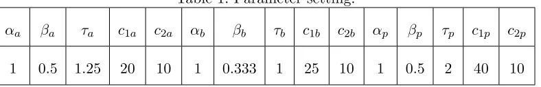
Table 1: Parameter setting.
αa βa τa c1a c2a αb βb τb c1b c2b αp βp τp c1p c2p
1 0.5 1.25 20 10 1 0.333 1 25 10 1 0.5 2 40 10
block replacement, and periodic replacement policies. For example,c1aandc2aare the cost of
replacement for a failed item and the cost of replacement for a scheduled item, respectively.
Here, we assume that c1∗ > c2∗ as replacement due to an unexpected failure typically incurs
higher costs than scheduled replacement.
5.3 Using the bootstrap method
We assume ma=mb =mp = 10.
We use the bootstrap method proposed by Efron (1981). The idea of this method is to sample
data from the censored dataset and the uncensored dataset respectively, and then combine
the two sample sets as a new sample set. We obtain the estimated parameters with the given data and plot the cost and variance variation with respect to the replacement time Ta, Tb,
and Tp.
5.3.1 Independently optimising maintenance policies
Age replacement The results are ˆαa= 0.942 and ˆβa= 0.335. WhenTa = 0.80, the optimal
cost Ca(T|θ) = 20.1 is achieved and its associated variance V ar(Ca(T|θ)) = 2.02.
Block replacement The results are ˆαb = 1.0395 and ˆβb = 0.341. When Tb = 0.66, the
optimal costCb(T|θ) = 24.7 is achieved and its associated variance V ar(Ca(T|θ)) = 8.37.
Periodic replacement with minimal repair The results are ˆαp = 0.753 and ˆβp = 0.567.
When Tp = 0.63, the optimal costCp(T|θ) = 37.4 is achieved and its associated variance
V ar(Ca(T|θ)) = 9.6.
5.3.2 Collectively optimising maintenance policies
For the three options, we have the following results.
G(T) = 1076.2 is achieved.
Option 2 On the basis of the results of the three policies in Section 5.3.1, the variance in the
left hand-side of the inequality (11):m2
aVθ(Ca(Ta|θa))+m2bVθ(Cb(Tb|θb))+m2pVθ(Cp(Tp|θp)) =
100×(2.02 + 8.37 + 9.6) = 1999, which implies the following two situations.
• ifν is set to be smaller than 1999, the constraint in the inequality (11) should take effect on the objective function;
Let ν0 = 1744. When Ta = 0.81, Tb = 0.63 and Tp = 0.63, the optimal solution
G(T) = 825 is achieved. As can be seen, the valuesTa, Tb and Tp are not equal to those
values in the three policies in Section 5.3.1. This implies that the constraint takes effect.
• if ν is set to be larger than 1999, the constraint in the inequality (11) should not take effect on the objective function.
If we let ν0 = 2044. When Ta = 0.81, Tb = 0.68 and Tp = 0.63, the optimal solution
G(T) = 822 is achieved. As can be seen, the values Ta, Tb and Tp are the same values
as in the three policies in Section 5.3.1. This implies that the constraint does not take
effect.
Option 3 Let C0 = 822. When Ta = 0.81, Tb = 0.68 and Tp = 0.63, the optimal solution
G(T) = 1944 is achieved.
Let C0 = 922. When Ta = 0.81, Tb = 1.99 and Tp = 0.42, the optimal solution G(T) =
1095 is achieved.
5.4 Using the δ method
We set ma = mb = mp = 200, so we are considering maintenance policies for a large
organisation which applies the same policies to many systems. Of course, the uncertainties
due to parameter estimation in assumed mathematical models will have a more substantial
influence the larger the number of systems maintained is.
5.4.1 Independently optimising maintenance policies
Age replacement The results are ˆαa= 1.053,V(ˆαa) = 1.419, ˆβa= 0.469 ,V( ˆβa) = 0.219,
and covariance between parameters αa and βa is -0.0383. When Ta = 1.03, the optimal
cost Ca(T|θ) = 21.05 is achieved and its associated variance V ar(Ca(T|θ)) = 139.5.
0.112, and covariance between parametersαb andβb is 0.107. WhenTb = 0.63, the optimal
cost Cb(T|θ) = 22.37 is achieved and its associated variance V ar(Cb(T|θ)) = 216.00.
Periodic replacement with minimal repair The results are ˆαp = 1.0385 and ˆβp =
1.981. When Tp = 0.49, the optimal cost Cp(T|θ) = 41.04 is achieved and its associated
variance V ar(Ca(T|θ)) = 2.13.
5.4.2 Collectively optimising maintenance policies
On the three options, we have the following results.
Option 1 Let ρ = 0.001. When Ta = 0.84, Tb = 1.38 and Tp = 0.49, the optimal solution
G(T) = 25220 is achieved.
Option 2 On the basis of the results of the three policies in Section 5.3.1, the variance in the
left hand-side of the inequality (11):m2
aVθ(Ca(Ta|θa))+m2bVθ(Cb(Tb|θb))+m2pVθ(Cp(Tp|θp)) = 40000×(139.5 + 216.0 + 2.13) = 1.43052×10⁷, which implies the following two situations. • if ν is set to be smaller than 1.43052×10⁷, the constraint in the inequality (11) should
take effect on the objective function;
Let ν0 = 1.23×10⁷. When Ta = 1.01, Tb = 0.54 and Tp = 0.59, the optimal solution
G(T) = 17011 is achieved. As can be seen, the values Ta, Tb and Tp are not equal to
those values in the three policies in Section 5.3.1. This implies that the constraint takes
effect.
• if ν is set to be larger than 1.43052×10⁷, the constraint in the inequality (11) should
not take effect on the objective function.
Let ν0 = 1.53×10⁷. When Ta = 1.03, Tb = 0.63 and Tp = 0.49, the optimal solution
G(T) = 16891 is achieved. As can be seen, the values Ta, Tb and Tp are the same those
values in the three policies in Section 5.3.1. This implies that the constraint does not
take effect.
Option 3 Let C0 = 16891. When Ta = 1.03, Tb = 0.63 andTp = 0.59, the optimal solution
G(T) = 1.43×10⁷ is achieved.
Let C0 = 18891. When Ta = 0.47, Tb = 1.4 and Tp = 0.48, the optimal solution
5.5 Sensitivity analysis
In Option 1 in the above examples,ρis selected to balance the effect of the expected cost and the variance of the cost. If the variance is small, compared with the expected cost, a large ρ
is selected to highlight the influence of variance. If a small ρ is selected, the variance would have little influence on the optimal decision. On the other hand, if the variance is large, a
small ρ is selected to emphasize the effect of expected cost. Because with the δ method, the number of systems is 200; while with the bootstrap method, the number of systems is 10.
There exists a quadratic relationship between the total variance and the number of systems.
The total variance withδ method is much larger than that with bootstrap method, a smaller
ρ is selected. In reality,ρ may be selected on the basis of the attitude of the decision maker.
(a) (b)
[image:20.595.82.506.274.554.2](c) (d)
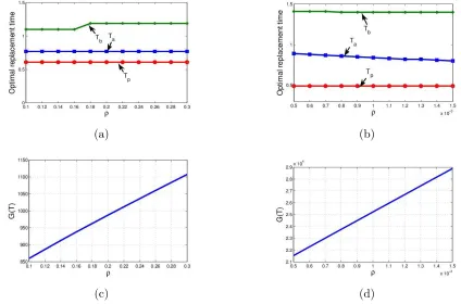
Fig. 1. Sensitivity analysis ofρ on the optimal decisions
The sensitivity analysis ofρ on the optimal decisions is shown in Figure 1. Optimal replace-ment time and maintenance cost is plotted with different ρ, with respect to the bootstrap method and δ method, respectively.
As shown in Figure 1, if ρ is increased towards 1, the objective function G(T) presents an increasing trend (See (c) and (d) in Figure 1) and the optimal maintenance time does
maintenance time is determined jointly by the expected cost rate function and the variance
function. As such, the relationship between the variance and maintenance time is not simply
monotonously decreasing or increasing.
6 Conclusions
This paper presents the first attempt to collectively optimise maintenance policies for a set
of different systems using the conditional value-at-risk theory, where model uncertainty is
explicitly considered in optimising maintenance policy. The proposed approaches can
espe-cially be beneficial to the asset management sector (or warranty suppliers), in which a large
number of different types of asset may be maintained and their reliability functions have different levels of efficiency. Collectively optimising preventive maintenance policies for each
asset can be more cost-effective.
This paper provides practitioners with alternative methods to optimise maintenance policies:
one can jointly optimise both the uncertainty of the expected cost of the maintenance policies
considered for a portfolio of assets and the expected cost. The selection among the three
options depends on decision maker’s risk attitude.
We briefly discuss some open questions and possible implications for asset management.
Risk aggregation. The above discussion uses the variance as a measure of risk. Many other
measures can also be applied. For example, the conditional value at risk (Rockafellar
& Uryasev, 2000), the mean absolute deviation approach of Konno & Yamazaki (1991),
the regret optimisation approach of Dembo & King (1992), and the minimax approach
of Young (1998) are notable, and can be applied in the context of maintenance policy
optimisation.
Adaptive preventive maintenance policy.As the above-mentioned, the reliability indexes are
assumed to be estimated based on failure data before the first PM time point. With time
development, more failure data can be collected and then fed into the model development.
As such, the efficiency of the estimators and the PM policy can be improved.
Maintenance policies. In this paper, only periodic PM policy is discussed. With more data
available over time, developing sequential PM policy is possible. Furthermore, one can also
Other uncertainty. In this paper, we considered model uncertainty. Other sources of
un-certainty may of course be taken into consideration. In developing maintenance policies
for either one-unit systems or complex systems, cost information is needed. In reality,
however, precise data on costs may not be available, which is especially true for complex
systems which includes many units and cost of repairing the units vary.
Acknowledgements
The authors are indebted to the reviewers for their constructive comments.
References
Aven, T. (2001). On the practical implementation of the Bayesian paradigm in reliability
and risk analysis. In Y. Hayakawa, T. Irony, & M. Xie (Eds.), System and Bayesian
reliability. Essays in honor of Professor Richard E. Barlow on his 70th birthday. (pp.
269–285). Singapore: World Scientific.
Barlow, R., & Proschan, F. (1965). Mathematical theory of reliability. New York: Wiley.
Coolen-Schrijner, P., & Coolen, F. (2006). On optimality criteria for age replacement.Journal
of Risk and Reliability, 220, 21–28.
Dembo, R. S., & King, A. J. (1992). Tracking models and the optimal regret distribution in
asset allocation. Applied Stochastic Models and Data Analysis, 8, 151–157.
Efron, B. (1981). Censored data and the bootstrap. Journal of the American Statistical
Association, 76, 312–319.
Fang, C., & Huang, Y. (2008). A Bayesian decision analysis in determining the optimal
policy for pricing, production, and warranty of repairable products. Expert Systems with
Applications,35, 1858–1872.
From, S. G., & Tortorella, M. (2005). Parametric confidence intervals for the renewal function
using coupled integral equations. Communications in Statistics: Simulation and
Compu-tation, 34, 663–672.
Guo, H., & Pan, R. (2008). On determining sample size and testing duration of repairable
system test. In Wu (Ed.),Proceedings - Annual Reliability and Maintainability Symposium
Hu, J., & Zhang, L. (2014). Risk based opportunistic maintenance model for complex
me-chanical systems. Expert Systems with Applications, 41, 3105–3115.
Jiang, R. (2010). A simple approximation for the renewal function with an increasing failure
rate. Reliability Engineering & System Safety, 95, 963–969.
de Jonge, B., Klingenberg, W., Teunter, R., & Tinga, T. (2015). Optimum maintenance strategy under uncertainty in the lifetime distribution. Reliability engineering & system
safety, 133, 59–67.
Konno, H., & Yamazaki, H. (1991). Mean-absolute deviation portfolio optimization model
and its application to tokyo stock market. Management Science,37, 519–531.
Krinsky, I., & Robb, A. L. (1986). On approximating the statistical properties of elasticities.
The Review of Economics and Statistics, (pp. 715–719).
Krokhmal, P., Zabarankin, M., & Uryasev, S. (2011). Modeling and optimization of risk.
Surveys in Operations Research and Management Science, 16, 49–66.
Laggoune, R., Chateauneuf, A., & Aissani, D. (2010). Impact of few failure data on the
opportunistic replacement policy for multi-component systems. Reliability Engineering
and System Safety, 95, 108–119.
Lin, S., & Bier, V. (2008). A study of expert overconfidence. Reliability Engineering and
System Safety, 93, 711–721.
Moghaddass, R., Zuo, M. J., Liu, Y., & Huang, H. Z. (2015). Predictive analytics using a
nonhomogeneous semi-markov model and inspection data. IIE Transactions,47, 505–520.
O’Hagan, A., & Oakley, J. E. (2004). Probability is perfect, but we can’t elicit it perfectly.
Reliability Engineering and System Safety, 85, 239–248.
Percy, D. F., Kearney, J. R., & Kobbacy, K. A. H. (2010). Hybrid intensity models for
repairable systems. IMA Journal Management Mathematics, 21, 395–406.
Rockafellar, R. T., & Uryasev, S. (2000). Optimization of conditional value-at-risk. Journal
of Risk, 2, 21–42.
Sirvanci, M., & Yang, G. (1984). Estimation of the weibull parameters under type i censoring.
Journal of the American Statistical Association,79, 183–187.
Speirs-Bridge, A., Fidler, F., McBride, M., Flander, L., Cumming, G., & Burgman, M.
(2010). Reducing overconfidence in the interval judgments of experts. Risk Analysis, 30,
512–523.
Wang, H. (2002). A survey of maintenance policies of deteriorating systems. European
Weisberg, S. (2014). Applied linear regression. New Jersey: John Wiley & Sons.
Wu, D., Zhou, J., & Li, Y. (2006). Methods for estimating weibull parameters for brittle
materials. Journal of Materials Science, 41, 5630–5638.
Wu, S., & Scarf, P. (2015). Decline and repair, and covariate effects. European Journal of
Operational Research, 244, 219–226.
Young, M. (1998). A minimax portfolio selection rule with linear programming solution.
Management Science, 44, 673–683.
Zhang, N., & Yang, Q. (2015). Optimal maintenance planning for repairable
multi-component systems subject to dependent competing risks. IIE Transactions,47, 521–532.
Zhu, B., & Frangopol, D. (2013). Risk-based approach for optimum maintenance of bridges
under traffic and earthquake loads. Journal of Structural Engineering (United States),
139, 422–434.
Z¨ornig, P. (2014). Nonlinear Programming: An Introduction. Berlin: Walter de Gruyter &
Appendix
Proof of Property 1.
Set the derivatives of G(T) in respect to Ta,Tb, and Tp to zero, respectively, and obtain
∂Ca(Ta|θa)
∂Ta
+ρma
∂Vθ(Ca(Ta|θa))
∂Ta
= 0 (34)
∂Cb(Tb|θb)
∂Tb
+ρmb
∂Vθ(Ca(Tb|θb))
∂Tb
= 0 (35)
∂Cp(Tp|θp)
∂Tp
+ρmp
∂Vθ(Cp(Tp|θp))
∂Tp
= 0 (36)
Plugging Eq. (1) into Eq. (34), one has
(ca1−ca2)ra(Ta|θa)
Z Ta
0
¯
Fa(t|θa)dt−(ca1 −ca2)Fa(Ta|θa)
=ca2−µma
dVθ(Ca(Ta|θa)) dTa
h RTa
0 F¯a(t|θa)dt
i2
¯
Fa(Ta|θa)
(37)
where ra(Ta|θa) represents the failure rate fa(Ta|θa)/F¯a(Ta|θa).
If one further assumes that ra(Ta|θa) is continuous and increasing, the left side of Eq. (37)
is continuous and increasing. Since both Vθ(Ca(Ta|θa)) and
hRTa
0 F¯a(t|θa)dt
i2
/F¯a(Ta|θa) are
increasing in Ta, the right side of Eq. (37) is decreasing. The minimum value of the left side
is 0 (whenTa = 0) and the maximum value of the right side of Eq. (37) isca2 (whenTa = 0),
so there exists a solution T∗
a satisfying Eq. (37).
Similarly, substituting Eqs (2) and (3) into Eq. (35) and Eq. (36), respectively, one obtains
cb1m(Tb|θb)Tb−cb1M(Tb|θb) = cb2−ρmb
dVθ(Cb(Tb|θb))
dTb
Tb2 (38)
and
cp1λ(Tp|θp)Tp−cp1Λ(Tp|θp) = cp2−ρmp
dVθ(Cp(Tp|θp))
dTp
Tp2 (39) where m(.) is the renewal density function and λ(.) is the failure intensity function.
Similarly, one can prove that there exist solutions for Eq. (38) and Eq. (39).
This proves Property 1.
One can write the Lagrange function for the optimisation problem in Eqs (10) and (11) as:
L(T) =maCa(Ta|θa) +mbCb(Tb|θb) +mpCp(Tp|θp)
+µ(m2aVθ(Ca(Ta|θa)) +m2bVθ(Cb(Tb|θb)) +m2pVθ(Cp(Tp|θp))−ν0). (40)
Then, the first order necessary conditions for a solution in nonlinear programming to be
optimum, or the Karush-Kuhn-Tucker conditions (see Z¨ornig (2014), p. 72), are given by those equations shown in Eqs (12)—(15), and the following two inequalities:
m2aVθ(Ca(Ta|θa)) +m2bVθ(Cb(Tb|θb)) +m2pVθ(Cp(Tp|θp))≤ν0 (41)
µ≥0 (42)
Below we discuss the existence of possible solutions of the above conditions.
Case 1. µ= 0.
Conditions (12),(13), and (14) become
∂Ca(Ta|θa)
∂Ta
= 0 (43)
∂Cb(Tb|θb)
∂Tb
= 0 (44)
∂Cp(Tp|θp)
∂Tp
= 0 (45)
Solving equations (43), (44), and (45) is equivalent to finding the PM policy for each system respectively, and then checking whether the constraint in (41) holds or not.
Case 2. µ >0.
In this case, the optimisation problem becomes solving Eqs (12), (13), (14), and the
following equation:
m2aVθ(Ca(Ta|θa)) +m2bVθ(Cb(Tb|θb)) +m2pVθ(Cp(Tp|θp)) =ν0 (46)
Similar to the proof process in Property 1, from Eqs (43), (44) and (45), one can obtain
solutions T∗
a, T
∗
b and T
∗
p, which are functions of µ. Substituting T
∗
a, T
∗
b and T
∗
p into Eq.
(46), one can obtain an equation with respect to µ. If the equation can be solved, then optimum T∗
a, T
∗
b and T
∗
p can be obtained.
This proves Property 2.
IfC0 is large enough, the constraint shown in Eq. (17) can be ignored. Asm2aVθ(Ca(Ta|θa))+
m2
bVθ(Cb(Tb|θb)) +m2pVθ(Cp(Tp|θp)) is decreasing in Ta, Tb and Tp, its minimum can be
achieved ifTa, Tb andTp are infinity. This implies that no replacement is needed when C0 is
large enough.