An Analysis of VP8, a new video codec for the web

(1)

Rochester Institute of Technology

RIT Scholar Works

Theses Thesis/Dissertation Collections

11-1-2011

An Analysis of VP8, a new video codec for the web

Sean Cassidy

Follow this and additional works at:http://scholarworks.rit.edu/theses

This Thesis is brought to you for free and open access by the Thesis/Dissertation Collections at RIT Scholar Works. It has been accepted for inclusion in Theses by an authorized administrator of RIT Scholar Works. For more information, please [email protected].

Recommended Citation

(2)

An Analysis of VP8, a New Video Codec for the Web

by

Sean A. Cassidy

A Thesis Submitted in Partial Fulfillment of the Requirements for the

Degree of Master of Science

in Computer Engineering

Supervised by

Professor Dr. Andres Kwasinski

Department of Computer Engineering

Rochester Institute of Technology

Rochester, NY

November, 2011

Approved by:

Dr. Andres Kwasinski

R.I.T. Dept. of Computer Engineering

Dr. Marcin Łukowiak

R.I.T. Dept. of Computer Engineering

(3)

Thesis Release Permission Form

Rochester Institute of Technology

Kate Gleason College of Engineering

Title:

An Analysis of VP8, a New Video Codec for the Web

I, Sean A. Cassidy, hereby grant permission to the Wallace Memorial Library to

repro-duce my thesis in whole or part.

Sean A. Cassidy

(4)

Acknowledgements

I would like to thank my thesis advisors, Dr. Andres Kwasinski, Dr. Marcin Łukowiak,

and Dr. Muhammad Shaaban for their suggestions, advice, and support. This thesis could

not have been completed if it were not for their input.

I would like to thank my fianc´ee, Amanda Fischedick, for her advice, support, and

encouragement. If it were not for her, there would be no box plots in this thesis, and

would be worse overall.

Finally, I would like to thank my friends and family. Without the encouragement and

advice of my family, I would not be at R.I.T. completing my thesis now. No amount

of acknowledgement can express my gratitude at their ceaseless work and care to get

me to where I am today. I would like to specifically thank my friends: Robert Ghilduta,

Jonathon Szymaniak, and Frank Jenner. They are some of the smartest people I know, and

offered numerous suggestions and support. This thesis would not have been completed

(5)

List of Figures

2.1 A Flowchart of the Encoding Process . . . 20

2.2 Subblock Mapping to the Token Probability Table . . . 22

2.3 The area around a macroblock that will be intra-compressed . . . 27

2.4 An intra-predicted macroblock using vertical prediction . . . 27

2.5 An intra-predicted macroblock using horizontal prediction . . . 28

2.6 Luma Intra-prediction overview . . . 29

2.7 Scan Orders for Transformed Coefficients . . . 33

2.8 The pixels for simple loop filtering on a vertical block border . . . 37

2.9 The pixels for simple loop filtering on a horizontal block border . . . 37

2.10 Bidirectional Frames in H.264 . . . 46

2.11 Alternate Reference and Golden Frames in VP8 . . . 47

2.12 Segments and Slices . . . 49

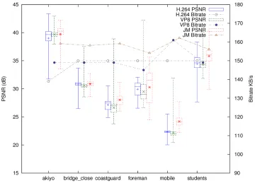
4.1 PSNR Summary of Videos at CIF, 150 Kbps, H.264 Baseline and VP8 Good Deadline . . . 81

4.2 SSIM Summary of Videos at CIF, 150 Kbps, H.264 Baseline and VP8 Good Deadline . . . 82

(9)

4.4 SSIM Summary of Videos at CIF, 150 Kbps, H.264 High Profile and VP8

Best Deadline . . . 83

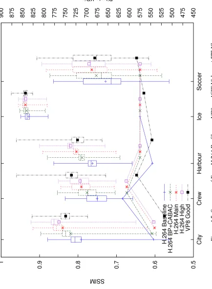
4.5 Summary of Four H.264 Profiles vs. VP8 on 4CIF Videos at 575 Kbps . . . . 88

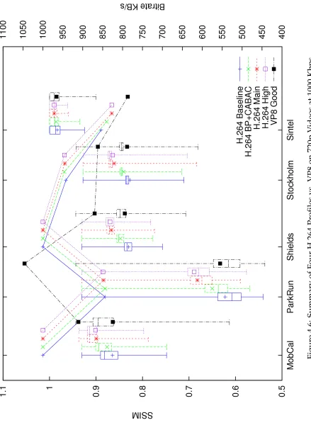
4.6 Summary of Four H.264 Profiles vs. VP8 on 720p Videos at 1000 Kbps . . . 89

4.7 Parkrun at 720p, encoded at 1000 Kbps . . . 90

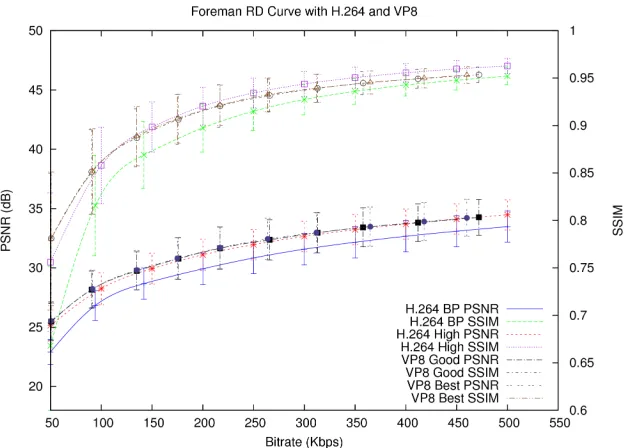
4.8 Foreman CIF Video RD Curve for H.264 and VP8 . . . 90

4.9 Soccer 4CIF Video RD Curve for H.264 and VP8 . . . 91

4.10 Stockholm 720p Video RD Curve for H.264 and VP8 . . . 91

4.11 Summary of Akiyo at CIF Resolution, 25 Kbps . . . 93

4.12 Frames of Akiyo at CIF Resolution, 25 Kbps . . . 93

4.13 Summary of Akiyo at CIF Resolution, 50 Kbps . . . 94

4.14 Frames of Akiyo at CIF Resolution, 50 Kbps . . . 95

4.15 Summary of Students at CIF Resolution, 25 Kbps, KF Interval 300 . . . 97

4.16 Frames of Students at CIF Resolution, 25 Kbps, KF Interval 300 . . . 97

4.17 Summary of Students at CIF Resolution, 25 Kbps, KF Interval 30 . . . 99

4.18 Frames of Students at CIF Resolution, 25 Kbps, KF Interval 30 . . . 99

4.19 SSIM Summary of the Three Videos at 720p, nominally 3000 kbps . . . 101

4.20 SSIM Frames of City Outdoors, 720p, nominally 3000 kbps . . . 102

4.21 SSIM Summary of the Three Videos at 1080p, nominally 5000 kbps . . . 103

4.22 SSIM Frames of Outdoor Pedestrians, 1080p . . . 105

4.23 SSIM Summary of In to Tree and Rush Hour . . . 106

4.24 SSIM Frames of In to Tree, 720p . . . 106

4.25 Bitrate vs. SSIM for H.264 Baseline and VP8 Good Deadline . . . 110

4.26 Bitrate vs. SSIM for H.264 High Profile and VP8 Best Deadline . . . 111

4.27 PSNR Summary of Inter-coding Tests . . . 113

(10)

4.29 Percent Difference for PSNR and SSIM among four resolutions for VP8 and

(11)

List of Tables

2.1 The Five Types of Motion Vectors . . . 31

3.1 Versions of the Software Used . . . 60

3.2 Source Videos at352×288Used and their Attributes . . . 61

3.6 Initial Testing Encoder Parameters . . . 67

3.7 Feature Set Testing Encoder Parameters . . . 67

3.8 Video Conferencing Encoder Parameters, from Slowest Encoding Speed to Fastest . . . 70

3.9 Source Videos for 720p Composite Films . . . 71

3.10 Source Videos for 1080p Composite Films . . . 72

3.11 Intra-coding Test Encoder Profiles and Parameters . . . 74

3.12 Configurations for Inter-coding Tests . . . 76

3.13 Configurations for Two Pass Loop Filter Tests . . . 79

4.1 p-values for RD Curve for Foreman . . . 86

4.2 p-values for RD Curve for Soccer . . . 86

(12)

4.4 p-values for Frames for the Fastest and Slowest Profiles for Akiyo at 25 Kbps 95

4.5 p-values for Frames for the Fastest and Slowest Profiles for Akiyo at 50 Kbps 96

4.6 p-values for Frames for the Fastest and Slowest Profiles for Students at 25

Kbps, 300 KF Interval . . . 98

4.7 p-values for Frames for the Fastest and Slowest Profiles for Students at 25 Kbps, 30 KF Interval . . . 100

4.8 p-values for the Average PSNR and SSIM Values based onσ . . . 109

4.9 Average Percent Difference for the four Resolutions and Overall . . . 115

B.1 p-values for SSIM Frames of City Outdoors, 720p . . . 135

B.2 p-values for SSIM Frames of Outdoor Pedestrians, 1080p . . . 135

B.3 Raw PSNR Values for Ice for Inter-Coding Test . . . 136

B.4 Raw SSIM Values for Ice for Inter-Coding Test . . . 136

B.5 Raw PSNR Values for Parkrun for Inter-Coding Test . . . 137

(13)

Abstract

Video is an increasingly ubiquitous part of our lives. Fast and efficient video codecs are

necessary to satisfy the increasing demand for video on the web and mobile devices.

However, open standards and patent grants are paramount to the adoption of video

codecs across different platforms and browsers. Google On2 released VP8 in May 2010

to compete with H.264, the current standard of video codecs, complete with source code,

specification and a perpetual patent grant.

As the amount of video being created every day is growing rapidly, the decision of

which codec to encode this video with is paramount; if a low quality codec or a

restric-tively licensed codec is used, the video recorded might be of little to no use. We sought

to study VP8 and its quality versus its resource consumption compared to H.264 – the

most popular current video codec – so that reader may make an informed decision for

themselves or for their organizations about whether to use H.264 or VP8, or something

else entirely.

We examined VP8 in detail, compared its theoretical complexity to H.264 and

mea-sured the efficiency of its current implementation. VP8 shares many facets of its design

with H.264 and other Discrete Cosine Transform (DCT) based video codecs. However,

VP8 is both simpler and less feature rich than H.264, which may allow for rapid hardware

and software implementations. As it was designed for the Internet and newer mobile

de-vices, it contains fewer legacy features, such as interlacing, than H.264 supports.

To perform quality measurements, the open source VP8 implementation libvpx was

used. This is the reference implementation. For H.264, the open source H.264 encoder

x264 was used. This encoder has very high performance, and is often rated at the top of

its field in efficiency. The JM reference encoder was used to establish a baseline quality

(14)

Our findings indicate that VP8 performs very well at low bitrates, at resolutions at and

below CIF. VP8 may be able to successfully displace H.264 Baseline in the mobile

stream-ing video domain. It offers higher quality at a lower bitrate for low resolution images due

to its high performing entropy coder and non-contiguous macroblock segmentation.

At higher resolutions, VP8 still outperforms H.264 Baseline, but H.264 High profile

leads. At HD resolution (720p and above), H.264 is significantly better than VP8 due to

its superior motion estimation and adaptive coding. There is little significant difference

between the intra-coding performance between H.264 and VP8. VP8’s in-loop deblocking

filter outperforms H.264’s version. H.264’s inter-coding, with full support for B frames

and weighting outperforms VP8’s alternate reference scheme, although this may improve

in the future. On average, VP8’s feature set is less complex than H.264’s equivalents,

which, along with its open source implementation, may spur development in the future.

These findings indicate that VP8 has strong fundamentals when compared with H.264,

but that it lacks optimization and maturity. It will likely improve as engineers optimize

VP8’s reference implementation, or when a competing implementation is developed. We

(15)

Glossary

4CIF Common Interchange Format, a format for broadcast video. Used in this thesis to

refer to704×576resolution.

ASIC Application Specific Integrated Circuit.

ASO Arbitrary Slice Ordering, a method in the H.264 standard to order slices in any

order

AVC Advanced Video Coding, part of the H.264 standard

BER Bit error rate, the percentage of bits in a stream that are in error.

CABAC Context-Adaptive Binary Arithmetic Coding, part of the H.264 standard to

losslessly compress residue.

CAVLC Context-Adaptive Variable Length Coding, part of the H.264 standard to

loss-lessly compress residue. Simpler than CABAC, but lower performing.

CIF Common Interchange Format, a format for broadcast video. Used in this thesis to

refer to352×288resolution.

DC Direct current, although used in this thesis and other works to refer to 0 Hz

fre-quency data

DCT Discrete Cosine Transform, a common method in image and video coding to get

(16)

FMO Flexible Macroblock Ordering, a method in the H.264 standard to allow

mac-roblocks that are not next to each other to share the same slice

HEVC High Efficiency Video Coding, the successor to H.264, slated for release in 2013.

HVS Human Visual System

Macroblock A square group of pixels. In this thesis, this exclusively refers to an8×8 macroblock of16pixels.

MP4 A file type that contains video and audio streams, also known as a container. Part

of the MPEG-4 standard.

MPEGLA The MPEG Licensing Authority

PSNR Peak Signal-to-Noise Ratio, a measure of quality, measured in decibels (dB).

NAL Network Abstraction Layer, part of the H.264 standard. This standardizes the

network representation of H.264 and adds network-aware features.

SSIM Structural Similarity, a measure of quality, measured from 0 to 1.0, where 1.0 is

perfect lossless quality.

SVC Scalable Video Coding, part of the H.264 standard, wherein the network video

stream degrades gracefully with packet loss and packet error

TCO Total Cost of Ownership, a measure of how expensive a technology is, including

(17)

VHDL VHSIC Hardware Description Language.

WHT Walsh-Hadamard Transform, another transform, similar to the DCT, to represent

data in the frequency domain

Y4M YUV for MPEG, a format for representing video in a raw format, with no loss of

quality or compression.

YCrCb Stands for the luminance, chroma red, and chroma blue color space. Widely

used in image and video processing.

(18)

Chapter 1

Introduction

Video coding is a complex topic, and seeks to appease the diverse group of video

con-sumers: from people watching short clips on smartphones to real-time video

conferenc-ing, to professional film studios and television broadcasters.

This chapter introduces what this thesis attempts to address, related work, an overview

of video coding including its various components, such as color and transformations.

1.1

Scope of this Thesis

This thesis covers VP8 and its implementation at the time of this writing. When

con-sidering which codec to use, many factors must be weighed, including the ease of use,

performance, and total cost of ownership (TCO), which includes possible legal fees

re-sulting from licensing or patent litigation. One particular codec may perform better than

another, but if the TCO is outside of the available budget, it cannot be considered.

Fur-ther, one must consider how easy it is for one’s organization to switch codecs; an online

video service cannot easily switch millions of videos without millions of hours of effort

(19)

switch the encoder they use in their products with relative ease.

VP8 was developed by On2 Technologies, later bought by Google Inc., to provide high

quality video for the web and mobile devices. It has a perpetual patent grant – something

which gives the implementor a no-charge, royalty-free, irrevocable patent license to use

or sell VP8, and the official reference implementation is open source. This thesis will not

cover estimated patent license cost, TCO, or legal implications of using VP8 over H.264

or vice versa. It will cover an objective analysis of the claims made by Google about VP8,

specifically with respect to its computational complexity and performance.

To analyze VP8 effectively, tests were designed to measure how each vital feature of

VP8 compares to a similar feature in H.264, as well as how each performs overall and

in several use case scenarios. A recommendation is made for improving VP8’s

imple-mentation, and recommends which codec to use for which purposes if legal and TCO

implications are not a factor. Not every use case or feature is possible to test, and there is

room for further analysis and recommendations.

For the purpose of this thesis, H.264 indicates H.264/AVC. H.264/SVC was not

ana-lyzed in detail, although some discussion of some of its features and how they compare to

VP8 are mentioned. Work on comparing VP8 to H.264/SVC has been studied by Seeling

et. al[1], and is not duplicated here.

The general method for comparing VP8 and H.264 is to analyze the components that

define the codecs, design methodology to compare these individual features, and run

tests on a varied set of source videos to gain an accurate understanding of how each

com-ponent compares to its counterpart in the other codec. By analyzing the codec by parts,

rather than by the whole, emphasis can be placed on where optimization should take

place. This also gives a more detailed view on the codecs, and can ignore

(20)

1.2

Related Work

A comparison between VP8 and H.264/SVC was performed by Seeling et. al, wherein

rate-distortion performance was compared with H.264 when there is significant traffic

variability on long video sequences[1]. Their conclusion was that VP8’s performance

was slightly less than H.264 SVC’s performance in this domain. They also state the

oft-repeated claim that On2, before it was sold to Google, claimed that VP8 offered twice the

quality of H.264 at half its bandwidth.

Another study compared VP8 to H.264 and HEVC – the next evolution of H.264, which

is planning to be standardized in 2013 – and found that, when 18 subjects viewed

vari-ous videos, that VP8 was competitive with H.264, specifically, the open source encoder

x264[2]. They used the 1080p source videos CrowdRun, DucksTakeOff, InToTree,

Old-TownCross, and ParkJoy from the VQEG HDTV SVT Dataset, and reduced their

resolu-tion to854×480and reduced their frame rate to 25 FPS. VP8 was not able to encode at very low bitrates – instead it would use a higher bitrate than requested; these bitrates were 250

kbps and 500 kbps. Overall, VP8 fared worse than x264, JM – the reference

implementa-tion of H.264/AVC, and HM – the test implementaimplementa-tion of HEVC, but the difference could

be due to the standard error within the video.

A technical summary of VP8 was published by the principal authors of VP8[3]. It

details the features that VP8 has in transformations, quantizations, its various reference

frame types, filtering, and its boolean entropy coding. The summary also includes

ex-perimental results, such as VP8’s impressive decoding speed, where VP8 achieves an

approximately40%faster decoding speed when compared to H.264. When using PSNR,

the RD curves presented in the summary for the videos HallMonitor, Highway,

Pam-phlet, and Deadline are nearly identical between VP8 and H.264. VP8 leads in the videos

(21)

There is some literature related to VP7, the previous iteration of VP8[4]. Their findings,

when VP7 was compared to H.264/SVC – the scalable video coding subset of H.264, was

that VP7 outperformed H.264/SVC on ADSL2+, HSDPA, WiMAX, and Ethernet LAN

networks for PSNR. However, H.264/SVC outperformed VP7 for the MOS, where five

people viewed the videos. Their sample size of five for the subjective video analysis is

small, and renders statistical analysis of their findings tenuous.

Surveys of H.264 have used PSNR [5, 6, 7] in comparing H.264 versus other codecs,

such as XviD, DivX, and Windows Media Codec 9. Some have used SSIM to measure

H.264 performance[8, 9, 7], while others have used lesser known metrics such as the JND

(Just Noticeable Difference)[5] or VQM (Video Quality Metric) [9, 7]. While it is shown

that PSNR and SSIM match the MOS values linearly[10], many studies also test MOS with

a small group of people[4, 11, 7]. For this thesis, PSNR and SSIM were chosen, as they are

popular, well tested metrics. MOS was also used for the subjective analysis portion.

H.264 was chosen as the sole codec to measure VP8 against, due to it outperforming

all other modern video codecs[5, 7]. This alleviates the need to test a large number of

codecs. x264 was chosen as the primary implementation of H.264 due to it being open

source, freely available for many platforms, and for its performance. It is faster than the

standard JM reference implementation by a factor of50, and outputs a bitstream withing

5%of the JM implementation for the same PSNR[12].

1.3

Overview of Video

Video is an significant part of modern life, from movies and television shows, to news,

sports, home videos and events. The Internet has been expanding in bandwidth usage at

an enormous rate, and Internet video tops the growth demographics. In late 2010, Cisco

(22)

on the Internet. Internet traffic increased 45.6% from 2008 to 2009, totaling approximately

176,200 petabytes (176.2 exabytes) for 2009. [13] The largest category of growing Internet

traffic is video to both personal computers, and TVs. Cisco predicts that Internet video

will occupy over 23,000 petabytes (23 exabytes) of the total Internet traffic in 2014, more

than half of the total bandwidth.

Dominating the video realm is the de-facto standard H.264, which is used on an array

of huge Internet video websites, from YouTube to Facebook. It offers a high peak

signal-to-noise ratio (PSNR) at a low bit-rate, and has several modes related to error mitigation

and error concealment. [14] A great deal of research has been created to improve H.264’s

error control and response mechanisms [15].

However, H.264, despite being an open standard, is protected by a myriad of software

and algorithmic patents in dozens of countries [16]. Some of these patents do not expire

until 2028, and this stifles the complete adoption of H.264, especially in the flourishing

open source community. In response, Google On2 released a competing video codec,

named VP8, in May of 2010. It is designed to be used as a general purpose codec for

streaming videos over the Internet, in a container known as WebM.

VP8 is designed to be simpler than H.264, and as such contains fewer color modes,

less available transformation sizes, a simpler loop filter; all while delivering a similar

bit-rate and visual quality to the end user. H.264’s complexity results in an efficient bitstream

that is already well supported by both hardware and software platforms. It will need to

be seen if VP8’s deviations will result in a quality video codec.

1.3.1

Color

Video formats that need to deal with color need to represent this information in a compact

(23)

– at the expense of increased algorithmic complexity required to subsample – to represent

an image. Generally, the technique is using a smaller resolution mapped to by copying

chroma pixels onto their respective luma counterparts, which are at a larger resolution.

The format is generally as shown in Eq. 1.3.1. rk-Usage Changes Push Internet Traffic to

the Edge

J :a :b (1.3.1)

This uses the notion of a reference block ofJpixels wide, and2pixels high.Jis almost always4. The valuearepresents the number of chroma blue, or Cb (which is a digitized chrominance sample of U) values overJand the valuebrepresents the number of chroma red, or Cr (which is a digitized chrominance sample of V) values overJ. [17]

However, the very common value 4:2:0, which is indeed what VP8 uses as its only

chroma subsampling technique, does not follow the convention shown in Eq. 1.3.1. For

purposes of this document, 4:2:0 will signify a chrominance pixel, comprising of both Cb

and Cr, that is at half the resolution of the luma pixel. Four luma pixels will map to a

single chrominance value.

Representing one of several millions of colors for every single pixel, known as the

4:4:4 image format, requires a large amount of space, but represents the color information

without loss of data.

1.3.2

Transforms

There are two main types of Fourier-class transforms used in modern video codecs. One

is the discrete cosine transform (DCT) and the other is the Walsh-Hadamard transform

(24)

The Discrete Cosine Transform

The DCT transforms a signal from the time domain to the frequency domain. As the

human visual system (HVS) is less sensitive to high frequency information, the high

quency components are discarded as they are less important than the DC and lower

fre-quency components. The formal definition of the4×4pixel DCT is shown in Eq. 1.3.2[18]. VP8 does not utilize this form directly; instead, it uses a one dimensional version with

multiple passes. In addition, VP8 is dissimilar to many other video codecs in that it uses

only a4×4transform. Other codecs also use a8×8transform or a16×16transform.

F (u, v) = 1 4CuCv

3 X i=0 3 X j=0

f(i, j) cos

π

4

i+1 2 u cos π 4

j+ 1 2

v

(1.3.2)

The inverse DCT is shown in Eq. 1.3.3:

f(i, j) =CuCv

3 X i=0 3 X j=0

F(u, v) cos

π

4

i+1 2 u cos π 4

j+ 1 2

v

(1.3.3)

The valuesCu andCv are scaling coefficients defined in Eq. 1.3.4:

Cx =        1 √

2 ifx= 0

1 otherwise

(1.3.4)

The Walsh-Hadamard Transform

The WHT, also known as the Hadamard Transform, is recursively defined as seen in Eq.

(25)

Hm = 1

√

2 

 

Hm−1 Hm−1

Hm−1 −Hm−1





 (1.3.5)

To transform a matrix via the WHT, the matrix,A, is multiplied byHm.Amust also be

a2m ×2m matrix. Eq. 1.3.6 shows the resulting transformed matrix, AW HT. This matrix

transformation, however, hasO(n2)complexity. There exists a fast WHT algorithm that usesnlognoperations[19].

AW HT =HmA (1.3.6)

1.3.3

Entropy Coding

The final step of video coding is entropy coding, which compresses data without

remov-ing entropy, or removremov-ing information. Messages, in the case of video, data, have a

partic-ular amount of unpredictability, known as entropy. The lower the entropy

(unpredictabil-ity) the easier the information is to represent using less data, known as compression. The

higher the entropy in the message, the lower the compression efficiency of the message

is. In video coding, the lower the entropy of the residue – what is left over after

transfor-mation – the higher the efficiency of the entropy coder.

Huffman coding and arithmetic coding are two ways in which lossless coding –

an-other term for entropy coding – is performed. Huffman coding is conceptually simpler,

but arithmetic coding is more efficient.

Huffman Coding

Huffman coding is used throughout VP8 to compress information about the data, such as

(26)

for the sub-block in question.

Huffman coding ranks symbols in descending order or their likeliness to appear in the

data stream. Higher probability symbols are given mappings to numbers with less bits,

to achieve high compression performance.

Arithmetic Coding

Arithmetic coding is a type of entropy coding that can achieve high levels of compression,

given certain information about the input domain. Arithmetic coding is similar to

Huff-man coding, which is another type of entropy coding, but instead of replacing each input

symbol into its own code, arithmetic coding replaces the entire message into a numbern, wheren∈[0.0,1.0].

Arithmetic coding operates by defining a probability model, similar to Huffman

cod-ing, and ranks input symbols according to how likely they are. The optimal value is

−log₂(P)bits for symbols of probabilityP.

After determining the probability of each input symbol, the intervals for each symbol

can be defined. If there are three symbols,Awith probability70%,Bwith probability20%, andCwith probability10%, then the three intervals are, respectively,[0,0.7),[0.7,0.9), and [0.9,1.0).

To encode a message to send, calculate the number n by subdividing the intervals to narrow the possibilities for messages. If the message isCAB, then the first interval is [0.9,1.0). Dividing this into three pieces of the probabilities specified in the previous para-graph results in three new intervals, A ∈ [0.9,0.97), B ∈ [0.97,0.99), and C ∈ [0.99,1.0). The next symbol isA, so that interval is chosen.

Dividing that interval into three pieces for the final symbol results in the three

(27)

but it is common practice to use the lower bound. Our message can then be represented

asn = 0.949. Neither floating point numbers, nor infinite precision is used to represent 0.949; rather, a fixed precision is used to limit the number of bits necessary to represent this number.

To decode a message received, the intervals need to be subdivided over and over

to reveal each symbol of the message, essentially the reverse of the encoding step. The

example message hasn = 0.949, which lies first in the interval for C, therefore the first symbol isC. The range forCwould be then subdivided as before, until revealing that the next symbol must beA, and then after subdividing that range, the final symbol,B.

VP8 uses arithmetic coding as its lossless coding, to compress the residue after

quan-tization, transformation, and prediction.

1.4

Objective Quality Measurements

There are many quantitative quality metrics for use with two-dimensional digital signals.

PSNR is an important metric, and is used often. However, there are important limitations

to using PSNR as a metric for measuring relative quality of encoded video. Comparing

the results from one raw input video to various encodings from the same encoder

pro-duces a strongly correlated result with respect to standard subjective testing. However,

across different videos, encoders, and even frame rates, PSNR is not an accurate

mea-surement [10]. Due to this, PSNR will only be utilized to measure relative gain within

one codec and within one source video only.

Recently, the structural similarity (SSIM) metric has become popular, and is claimed to

better capture the psycho-visual perception of humans, based upon the HVS model [20].

These two popular metrics will be used in the evaluation of VP8 due to their support and

(28)

(VQM) and the HVS Similarity Measure (HSM) [9] were considered for the evaluation,

but did not offer substantial benefits when compared to PSNR and SSIM.

The standard metric for analyzing the differences between any two digital data streams

is the PSNR. The PSNR for video is defined as in Eq. 1.4.1 b[18]. The valuexis the max-imum value a pixel can be in imageA andB. For a 16-bit grayscale image, this value is

65535. The Mean Square Error (MSE) is used as shown in Eq. 1.4.1 a, for grayscale images.

mrefers to the number of rows in a matrixAm,n, wherenis the number of columns.

M SE = 1

mn

m−1

X

i=0

n−1

X

j=0

(A(i, j,)−B(i, j))2 (1.4.1a)

P SN RdB = 10 log10

x2

M SE (1.4.1b)

SSIM is defined in terms of mean luminance intensity for an image A, Eq 1.4.2 a, the signal contrast, using the standard deviation as an estimate, Eq 1.4.2 b, to form the SSIM

calculation as seen in Eq. 1.4.2 c [20]. C1 is a constant defined as C1 = (K1L)2, which is

used to avoid situations where the square sum of the mean luminance intensities is near

zero.Lis the highest value of a pixel, similar toImaxfor PSNR, andK1 1. C2 is similar

toC1and is defined asC2 = (K2L)2, whereK2 1.

µA= 1

N

N X

i=1

Ai (1.4.2a)

σA= v u u t

1

N −1 N X

i=1

(Ai−µA)2 (1.4.2b)

SSIM(A, B) = (2µAµB+C1) (2σAB+C2) (µ2

A+µ2B+C1) (σ2A+σB2 +C2)

(29)

In general, both PSNR and SSIM are sensitive to similar noise and errors in images[21].

Using two similar metrics in this thesis gives a more complete picture of the codecs under

study.

This chapter addressed the goals of and work related to this thesis. It examined much

of the background material necessary to accurately follow the remainder of this document

and to have a full understanding of the implications thereof.

The next chapter will introduce VP8 as a video codec, which will examine it at a high

(30)

Chapter 2

VP8 and H.264 Compared

VP8, the video codec in the WebM media container released by Google Inc., in May 2010,

is a modern video codec with many advanced features designed to have a high visual

quality at a low bitrate. This chapter covers VP8 in detail, explaining its encoding process,

quantization, transformation, entropy coding, prediction, and filtering.

A direct comparison with H.264 is made, discussing inter-prediction differences,

adap-tive behavior – including segmentation and slices, quantization, transformations, and

en-tropy coding, and network streaming support. HEVC, the next video standard being

developed by the Joint Collaborative Team on Video Coding (JCT-VC), is introduced and

compared with VP8. The ease of implementation of VP8 in hardware is discussed, and

the reference hardware implementation is compared with implementations of H.264 in

hardware.

2.1

VP8 Internals

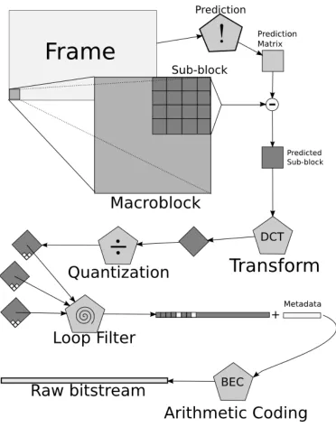
The encoding process of VP8 follows five steps in order. First, the macroblock to be

(31)

mac-roblock. Next, the macroblock is transformed, using either the DCT or the WHT,

depend-ing on the prediction mode. This is explained in Section 2.1.2. After transformation, the

quantization step takes the outputs of the transformation process, and restricts them to a

certain output range.

Figure 2.1 shows the encoding process. The output from the Prediction block is the

predictor, and is subtracted from the macroblock by value. The Prediction block uses

spatial information (pixel values surrounding the sub-block), and temporal information

(motion vectors from other frames). The Transform block uses the prediction mode to

decide whether or not to use the WHT or the DCT.

The predicted, transformed, and quantized macroblock is then run through the loop

filter, discussed in Section 2.1.7, and finally entropy encoded, as discussed in Section 1.3.3.

2.1.1

Quantization

Quantization is an signal processing technique where a continuous or large set of input

ranges are mapped to a discrete or smaller set of ranges. VP8, like many other video

codecs, uses quantization as a method for discarding superfluous data to enhance the

compression efficiency.

To quantize the residue, each coefficient is divided by one of six quantization factors,

the selection of which depends upon the plane being encoded. In VP8, a plane is a set

of two-dimensional data with metadata describing the type of that data. There are four

types of planes in VP8: Y2, the virtual plane from the WHT, Y, the luminance plane, U,

the chroma red plane, and V, the chroma blue plane. The quantization step also depends

upon the coefficient position, either DC – coefficient 0, or AC – coefficients 1 through 15.

These values are specified in one of two ways, via an index into a look-up table, or as an

offset to an index.

(32)

quan-Figure 2.1: A Flowchart of the Encoding Process

tizer lookup table. Yacis added to each of the other quantization factors, which are

speci-fied as 4-bit positive or negative offsets from the index ofYac.

Each other factor is specified as a four bit offset from theYacindex, and include a sign

[image:32.612.120.492.66.539.2]

(33)

bitstream, the five factors other thanYac are optional, and only included if a flag is true.

If they are omitted, they are set to zero, which indicates that the same quantization factor

asYac should be used for them.

To dequantize the residue before inverting the transform during decoding, each

coef-ficient is multiplied by one of six dequantization factors.

2.1.2

Transforms

The quantized DCT coefficients are coded for each macroblock, and they make up what

is known as the residue signal. The residue is added to the prediction blocks (either

Intra-prediction as described in Section 2.1.4 or Inter-Intra-prediction as described in Section 2.1.5) to

form the final reconstructed macroblock.

Unlike H.264, VP8 uses only4×4DCT and WHT for its transformations (see Sections 1.3.2 and 1.3.2 for more information). The DCT is used for the 16 Y sub-blocks of a

mac-roblock, the 4 U sub-blocks, and the 4 V sub-blocks. The WHT is used to construct a4×4 array of the average intensities of the 16 Y sub-blocks. This is a stand-in for the 0th _DCT

coefficients of the Y sub-blocks. This is known asY2_{, and is considered a}_virtual_subblock,

contrasted to the 24 other, real, sub-blocks. The subblock Y2_{is conditional, based upon}

the prediction mode.

The 4×4DCT in H.264 and VP8 can be computed with integer arithmetic only [22]. This enables it to operate quickly and with low complexity, as it avoids floating point

operations. Further, only 16-bit arithmetic is required for both the H.264 DCT and the

(34)

The Transformed Coefficients

The coefficients of the 16 sub-blocks of each macroblock are arithmetic coded, and are

known as “tokens”. The probability table for decoding this is four-dimensional, and is

dependent on the type of plane being decoded, the sub-block being decoded, the local

complexity, and the token tree structure.

There are four possible values for the first dimension of the probability table,

depend-ing on what type of plane is bedepend-ing decoded, either Y after a Y2 plane, a Y2 plane, a chroma

plane (U or V), or a Y plane without a Y2 plane, index, respectively from0to3.

The next dimension depends upon the position of the current subblock within the

current macroblock, and is indexed from 0to 7, known as bands. The mapping of sub-blocks to the index is shown in Figure 2.2. The upper half of the macroblock and the last

subblock are treated specially, while the lower half shares index6.

0 1 2 3

6 4 5 6

6 6 6 6

6 6 6 7

Figure 2.2: Subblock Mapping to the Token Probability Table

The local complexity dimension attempts to match the local area to the corresponding

probability. If there are many zeros in the local area, it is more likely that index0is used.

If there are some, but not a lot,1is used. If there is a large amount, index2is used.

For the first coefficient of the macroblock, the surrounding macroblocks are examined.

The index is the number of surrounding macroblocks that contain at least one non-zero

coefficient in their residue. This way, the first coefficient’s probability accuracy depends

on how similar it is to the immediately surrounding macroblocks.

For the remainder of the coefficients, the local complexity index is described by Eq.

(35)

This can have suboptimal behavior when wrapping around the macroblock, for instance,

from position3to position4.

As the meaning between the first and remaining coefficients is slightly different for the

local complexity dimension, it is important to note that this is acceptable, because each

subblock position maps to a band, as shown in Figure 2.2. Therefore, the first coefficient

has its own probabilities for the cases of surrounding macroblocks, and it doesn’t interfere

with the other meaning of local complexity, which is the value of the previous coefficient,

as described in Eq. 2.1.1.

ilc ←               

0 ifclast = 0 1 if |clast|= 1 2 if |clast|>1

(2.1.1)

Inverse DCT and WHT

Before dequantizing the DCT and WHT factors, the inverse transform must be performed.

If the Y2 block exists (if a prediction mode other than B PRED for intra- and SPLITMV for

inter-prediction is used), then it is inverted via the WHT.

The WHT is defined in Eq. 1.3.5, and is the inverse WHT is implemented in Alg.

1 on page 24, where input and output are arrays of signed 16-bit integers. This is an

O(nlogn)implementation of the Fast Walsh-Hadamard Transform, which uses an archi-tecture similar to the Cooley-Tukey algorithm for Fast Fourier Transforms[19]. There is

also an optimization if there is only one non-zero DC value in theinputarray. For the inverse DCT, two passes of a 1D inverse DCT is used.

Alg. 2 on page 41 is used to compute the inverse DCT. The two constantsf1andf2 are

typically expressed as 16-bit fixed-point fractions, and are given in the bitstream reference

(36)

Algorithm 14×4Inverse WHT

i←0

c←0

while i <4 do

a1 ←input[c+ 0] +input[c+ 12]

b1 ←input[c+ 4] +input[c+ 8]

c1 ←input[c+ 4] +input[c+ 8]

d1 ←input[c+ 0] +input[c+ 12]

output[c+ 0]←a1+b1

output[c+ 4]←c1+d1

output[c+ 8]←a1−b1

output[c+ 12]←d1−c1

i←i+ 1

c←c+ 1 end while

i←0

c←0

while i <4 do

b1 ←input[c+ 1] +input[c+ 2]

c1 ←input[c+ 1] +input[c+ 2]

d1 ←input[c+ 0] +input[c+ 3]

output[c+ 0]← 1

8(a1+b1+ 3)

output[c+ 1]← 1

8(c1+d1+ 3)

output[c+ 2]← 1

8(a1−b1 + 3)

output[c+ 3]← 1

8(d1−c1 + 3)

i←i+ 1

2.1.3

Boolean Entropy Encoder

The VP8 data stream is compressed via a boolean entropy encoder, which is a type of

arithmetic coder (see Section 1.3.3). For this type of arithmetic coding, there are only

two symbols,true_orfalse_{. The goal of VP8’s other steps, such as the DCT coefficient}

coding and prediction is to insert morefalsevalues thantruevalues, so that the

prob-ability of a false value is higher, thus increasing the efficiency of the boolean entropy

(37)

The equation for determining the smallest datarate per value is in Eq. 2.1.2, whereR

is measured inbits_/ value.

R=−plog₂(p)−(1−p) log₂(1−p) (2.1.2)

At the valuep = 1₂,R = 1bits_/

value, which is the worst case of the boolean entropy

en-coder. However, atp= ₁₁₆₃1 ,R= 0.01bits_/

value, which is substantially better than encoding

every single boolean.

Bit Representation of the Entropy Encoder

The probabilities that the boolean entropy encoder works with in VP8 are unsigned 8-bit

integers,p0. To get the actual probabilityp∈[0,1], the 8-bit integer is divided by256. The state of the encoder is maintained with five values, the current bit position n, the bit string already written, w, the bottom value, an 8-bit integer ibot, and the range,

another 8-bit integer, irng. The range is clamped to within a specified boundary, so that

the probabilities remain accurate,irng ∈[128,255].

The valuev is the next value ofw, and the final value ofvis the end condition, where

v =x. vmust satisfy the inequality in Eq. 2.1.3. The scale of the bit position 8-bits ahead is generated as,s = 2−n−8_{. Another value, split, is calculated as follows,}_split_{= 1 +}p0(irng−1)

256 ,

and is constrained,split∈[1, irng−1].

w+ (s ibot)≤v < w+ (s(ibot+irng)) (2.1.3)

The boolean value to be encoded, b, has a zero probability of ₂₅₆p0 , where p0 ∈ [1,255]. The process for encoding one boolean valueb into the outputwis shown in Alg. 3. This algorithm is repeated for each boolean value that must be encoded. This is parallelized in

(38)

To decode a boolean encoded by Alg 3, the decoding process described in Alg. 4 on

page 42 is used.

2.1.4

Intraframe Prediction

VP8 uses two types of prediction vectors to achieve high compression performance. The

simpler type is intra-prediction, where the frame is predicted from other components of

the already constructed frame. As macroblock prediction is resolved in raster-scan order,

intra-prediction generally works from the top left, to the bottom right.

Chroma Intraframe Prediction

Chroma intra-prediction works on the 8-by-8 blocks of both U and V chroma. The

com-ponents of intra-prediction are M, which is the 8-by-8 matrix of either U or V, as shown in Figure 2.3.

Ais the bottom row of the macroblock above the current macroblock M, and is 1-by-8. If M is currently in the topmost position, then the values of A are all 127. L is the rightmost right of the macroblock to the left of the current macroblockM, and is 8-by-1. IfM is currently in the leftmost position, then the values ofAare all129. P is a scalar, the bottom-rightmost chroma value from the macroblock above and to the left of the current

macroblockM. If M is currently in the topmost and leftmost position, then the value of

P is129.

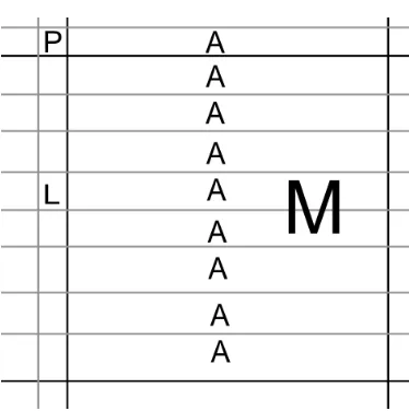
Vertical Prediction Vertical prediction, known as V PRED _{in the} libvpx _{source code,}

(39)

[image:39.612.213.401.300.499.2]

Figure 2.3: The area around a macroblock that will be intra-compressed

Figure 2.4: An intra-predicted macroblock using vertical prediction

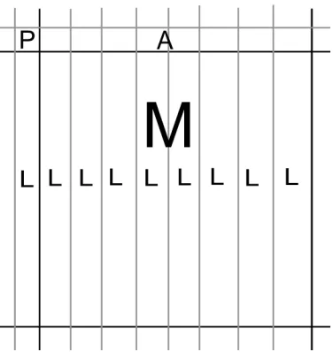
Horizontal Prediction Horizontal prediction, known asH PRED _{in the}libvpx_source

code, fills every8chroma row ofM withA. See Figure 2.5 for a graphical representation of horizontal prediction.

DC Prediction In DC prediction mode, known asDC PRED_{in the}libvpx_{source code,}

(40)

[image:40.612.212.399.64.252.2]

Figure 2.5: An intra-predicted macroblock using horizontal prediction

∀i∀j Mi,j = 1 16

8

X

k=1

Ak+ 1 16

8

X

l=1

Ll (2.1.4)

True Motion Prediction The True Motion prediction mode, known asTM PRED _{in the}

libvpxsource code, uses rowA, columnL, and chroma pixel P in its prediction. It as-signs chroma values according to the algorithm specified in Eq. 2.1.5, with the definition

ofClampj,k as specified in Eq. 2.1.6.

Mi,j =Clamp0,255(Lj +Ai−P) (2.1.5)

where

Clampj,k(x) =               

k ifx > k x ifj > x≥k j ifj ≥x

(41)

Luma Intraframe Prediction

The prediction process for Luma prediction is nearly identical to the chroma

intra-prediction methods, with the primary difference being that luma has a 16-by-16

tion matrix, while chroma is only 8-by-8. Luma intra-prediction has all the same

predic-tion methods that chroma intra-predicpredic-tion has (namely, vertical, horizontal, DC, and True

Motion prediction) with one additional prediction mode.

The luma-specific intra-prediction mode is comprised of intra-prediction on the four

4×4sub-blocks of the macroblockM. Each4×4sub-block can be independently intra-predicted via one of 10 sub-block intra-prediction modes. Figure 2.6 shows the many

possible components of luma intra-prediction.

Figure 2.6: Luma Intra-prediction overview

For subblock B1, the prediction mode may use the 8 pixel rowA1, which spans from

one pixel above the top left pixel of B1 to one pixel above the top right pixel of B2. It

also may useP1 the single pixel immediately to the left ofA1, orL1, which is the 4 pixel

(42)

Each one of the sub-blocks can use their own corresponding pixels to predict, as shown

in Figure 2.6. B2 may useA2, which stretches into the neighboring macroblockM2, orP2,

which is the fourth pixel from the left ofA1, orL2, which is the rightmost 4 pixel column

ofB1.

2.1.5

Interframe prediction

Interframe prediction is accomplished with a reference frame and offsets relative to the

reference frame, known as motion vectors. Motion vectors are vectors through three

di-mensions: two-dimensions in space, to show movement from one position in a frame to

another, and a third in time, to allow the motion to occur. Each macroblock for the current

frame is predicted using the 16 luma sub-blocks and the 8 chroma red and 8 chroma blue

sub-blocks.

Macroblocks in interframes can be coded. This can be used to provide

intra-refreshes between long key frames, where, at specific intervals, each interframe codes one

column of intra-coded macroblocks. These columns sweep from left to right, refreshing

the image as a fully coded key frame would.

Motion Vectors

Decoding the motion vectors will provide not only the sixteen Y sub-blocks with

individ-ual motion vectors, but it will also define the inter-prediction buffer. Like H.264, quarter

pixel (qpel) precision – explored in “Interpolation and Filtering” on page 31 – is

sup-ported by VP8.This is accomplished by interpolating between two pixels to get a median

value, and then interpolating between the median value and the two pixels to get quarter

median values.

(43)

used to decode the motion vectors is calculated via three neighboring macroblocks, top,

left, and top-left. For macroblocks on the topmost or leftmost edge, there are implicit

macroblocks with zero motion vectors. If a neighboring macroblock was intra-coded, it

does not factor in to the calculation.

Table 2.1: The Five Types of Motion Vectors

Name Description

Nearest Use the nearest MV for this MB Near Use the next nearest MV for this MB

Zero Use a zero MV for this MB

New Use an explicit offset from implicit MV for this MB Split Use multiple MVs for this MB

To determine the best, nearest and near motion vectors, an algorithm determines the

weight of the motion vector in question by examining surrounding macroblocks. Alg. 5

on page 43 shows the method by which this works. The functionf rametype(M) takes a macroblock and returns the prediction mode used. If Fintra is used, the algorithm will

skip the macroblock in question. The functionM V (M)returns the motion vector for the corresponding macroblock.

Interpolation and Filtering

Interpolation is used to achieve quarter pixel accuracy in the motion vector estimation

in VP8. Quarter pixel accuracy indicates that not only are individual pixels accessible

by motion vectors, but the space between pixels (half pixel accuracy), and the space one

quarter of the way between pixels. VP8 uses two types of FIR filters, bicubic filters for

higher quality estimation, and bilinear filters for reduced complexity estimation. The

bicubic filter has six filter coefficients (taps), and has eight preset filters, which are used

depending on the circumstance.

(44)

convo-lution. The process uses a clamped convolution, as shown in Eq. 2.1.7, which defines the

function if ilter. This convolution is used in both passes, the horizontal initial pass, and the final vertical pass, which uses theif iltervertvariant. The variant uses columns rather

than rows, and takes advantage of the fact that the width of thetemparray mentioned in Alg. 6 on page 44 is of width4.

if ilter(−→x , c) =Clamp0,255 3

X

c=−2

bc+2·x[c]

!

if iltervert(−→x , c) =Clamp0,255 3

X

c=−2

bc+2·x[4c]

! (2.1.7)

For the initial horizontal pass, nine rows of four interpolated values each are

calcu-lated, as shown in Alg. 6. The initial value, p, is used here not as a single scalar, but a scalar in a linear array of pixels. The functionif ilter references pixels before and after the given value. After the temp array of values is generated, the final vertical pass is performed, as shown in Alg. 7 on page 44.

Thef inalarray, is a two-dimensional array four pixels wide by four pixels tall, which contains the interpolated qpel values for the bottom right for the given pixel. The filter

taps, given in Eq. 2.1.7 as b, are predefined. The choices for bicubic interpolation are whole pixel (copies the given pixel), 1_/₈_, 1_/₄_, 3_/₈_{, symmetric} 1_/₂_, 5_/₈_, 3_/₄_{, and} 7_/₈_{. Bilinear}

pre-defined filters are also available for simpler encoding modes.

2.1.6

Scan Order

VP8 processes data in a predefined order, known as raster-scan order. This ordering

be-gins at the top left, and progresses from left-to-right and top-to-bottom, in the same way

that English is read. Figure 2.7b shows this scan order.

(45)

way, as in Figure 2.7b. As the transformed coefficients are most similar near the DC value,

and grow in both the X and Y dimensions in the same way, H.264 uses a zig-zag packing

method, as shown in Figure 2.7a.

This groups similar sized elements together for better lossless compression. This is

due to the way the two-dimensional DCT organizes its data. High frequency data is in

the bottom right, and lower frequencies radiate outwards. Snacking back and forth lumps

together similar coefficients for a lower entropy, and thus a higher compression efficiency.

H.264 also has field scan order for interlaced videos, but VP8 does not support

inter-laced videos.

(a) H.264’s Transformed Coefficient Scan Order for Progressive Frames

(b) VP8’s Transformed Coefficient Scan Order

Figure 2.7: Scan Orders for Transformed Coefficients

2.1.7

Loop Filter

As VP8 operates on 4×4macroblocks, there can be sharp contrast on the edge of two macroblocks. These aberrations can be unsightly, and need to be smoothed before the

final image is ready. This process is known as loop filtering. This isn’t merely a cosmetic

detail that the decoder does before producing a visible frame; its results are used for

(46)

As loop filtering is very computationally intensive, there are several types of filtering,

on the frame level and on the macroblock level. The frame header can select one of three

types, “none”, “simple”, and “normal”. Each macroblock, assuming that “none” was not

selected for this frame, can select its own loop filter that may be different than the frame

default loop filter.

There are two control parameters, the loop filter level, denotedFl, which can be

mod-ified on a per-macroblock basis, and the sharpness level, denoted Sl, which is constant

for a frame. The parameterFl is a threshold, which can denote that differences belowFl

are artifacts arising from compression, and therefore needs to be smoothed. Fl is

gener-ally related to quantization levels: the higher the quantization, the higherFlshould be to

smooth those anomalies out.

Construction of Thresholds and Parameters

The parameter Il, the interior limit, is a parameter used to calculate various thresholds.

Its derivation is seen in Eq. 2.1.8.

I_l0 ←

              

Fl/4 ifSl >4

Fl/2 ifSl >0

Fl otherwise

Il←       

9−Sl ifFl0 >9−SlandFl6=Il0

I_l0 otherwise

(2.1.8)

The loop edge thresholds, the macroblock edge thresholdEM B, and the subblock edge

(47)

EM B ←2 (Fl+ 2) +Il

ESB ←2Fl+Il

(2.1.9)

For high edge variance thresholds, the valueEHV is defined in Eq. 2.1.10.

EHV ←                               

2 if decoding key frame andFl≥40 1 if decoding key frame andFl≥15 3 if not decoding key frame andFl ≥40 2 if not decoding key frame andFl ≥20 1 if not decoding key frame andFl ≥15

(2.1.10)

Pixel Adjustment

If either of the loop filters determine that a set of edge pixels needs to be adjusted, then

a common adjustment routine is followed. This routine uses the Clampj,k function, Eq.

2.1.6 extensively.

First, the parametersA,A0, andBare set up in Eqs. 2.1.12 and 2.1.13. For convenience, Eq. 2.1.11 is used to shorten the notation to indicate the clamping of a signed byte.

CB(x) =Clamp−128,127(x) (2.1.11)

A0 ←

      

CB(CB(P1 −Q1) + 3 (Q0 −P0)) if using outer taps

3 (Q0−P0) if not using outer taps

A← A

0_{+ 4}

8

(48)

B ←

   

  

−1 if lower 3-bits of A’ = 4

0 otherwise

(2.1.13)

Then, the bordering pixels are adjusted using the parameters Aand B in Eqs. 2.1.14 and 2.1.15.

P₀0 ←P0+CB(A+B) (2.1.14)

Q0₀ ←Q0−A (2.1.15)

Simple Loop Filter

The primary focus of any macroblock loop filter is to reduce the difference in pixels along

an edge. To achieve this, the simple loop filter adjusts only the luma values, leaving the

chroma values unaffected. Differences in luma values aboveF_l00are assumed to be natural differences in the input video, while values below are assumed to be artifacts from the

compression process.

The simple filter operates on four luma pixels in either a row, if the edge is vertical,

or a column, if the edge is horizontal. The four pixels are termedP0, the pixel before the

edge,P1, the pixel preceding P0, Q0, the pixel after the edge, and Q1, the pixel after Q0.

See Figures 2.8 and 2.9 for a diagram of these border pixels. If the inequality in Eq. 2.1.16,

whereEis eitherEM B orESBdepending on the type of the current edge, is true, then the

pixels are adjusted. If the inequality is false, the pixels do not change.

E ≥2|P0−Q0|+

|P1−Q1|

(49)

M P1 P0 Q0 Q1

Figure 2.8: The pixels for simple loop filtering on a vertical block border

Q1

Q0

P0

P1

M

Figure 2.9: The pixels for simple loop filtering on a horizontal block border

Normal Loop Filter

Unlike the simple loop filter, the normal loop filter differs depending on whether the

edge is a macroblock or subblock edge. There are strong similarities between the two

algorithms, and they each use common algorithms for thresholding.

If every inequality of Eq. 2.1.17 is true, given the correct value of E (eitherEM B for

macroblocks orESB for sub-blocks), then the filtering is enabled. Otherwise, the filtering

is not used for this set of pixels.

Filtering depends on how severe the edge variance is, and Eq. 2.1.18 is used to

deter-mine if the current edge has high edge variance. If either inequalites of Eq. 2.1.18 are true,

(50)

E ≥2|P0−Q0|+

|P1−Q1|

2 (2.1.17)

Il≥ |P3 −P2|

Il≥ |P2 −P1|

Il≥ |P1 −P0|

Il≥ |Q3−Q2|

Il≥ |Q2−Q1|

Il≥ |Q1−Q0|

EHV <|P1 −P0|, (2.1.18)

EHV <|Q1−Q0|

Macroblock Edge Adjusment The process for determining whether the filter should

be enabled for macroblocks is as follows. If the inequalities in Eq. 2.1.17 are true, then

the inequalities in Eq. 2.1.18 are evaluated. If either is true, then the pixel adjustment

procedure is performed as described in Section 2.1.7 is used, with outer taps enabled.

If both inequalities of Eq. 2.1.18 are false (no high edge variance), then the pixels are

adjusted according to Eq. 2.1.19.

For convenience, Eq. 2.1.11 is used to shorten the notation to indicate the clamping of

(51)

W ←CB(CB(P1−Q1) + 3 (Q0−P0)) (2.1.19)

X00 ←CB

1

27 (27W + 63)

Q0 ←Q0−X00

P0 ←P0+X00

X0 ← 1

27CB(18W + 63)

Q1 ←Q1−X0

P1 ←P1+X0

X ← 1

27CB(9W + 63)

Q2 ←Q2−X

P2 ←P2+X

Subblock Edge Adjustment The process for determining whether the filter should be

enabled for sub-blocks is as follows. If the inequalities in Eq. 2.1.17 are true, then the

in-equalities in Eq. 2.1.18 are evaluated. If either is true, then the pixel adjustment procedure

is performed as described in Section 2.1.7 is used, with outer taps enabled.

If both inequalities of Eq. 2.1.18 are false (no high edge variance), then the pixel

ad-justment procedure described in Section 2.1.7 is used, with outer taps disabled. Then,

only if there was no high edge variance, pixelsP1 andQ1 are adjusted further. The pixels

(52)

P1 ←CB

P1+

A

2

, (2.1.20)

Q1 ←CB

Q1−

A

(53)

Algorithm 24×4Inverse DCT

f1 ←

√

2cos(π/8)−1

f2 ←

√

2sin(π/8)

i←0

c←0

spitch← pitch

2

while i <4 do

b1 ←input[c+ 0]−input[c+ 8]

t1 ←f2 ·input[c+ 4]

t2 ←input[c+ 12] + (f1·input[c+ 12])

c1 ←t1−t2

t1 ←input[c+ 4] + (f1·input[c+ 4])

d1 ←t1+t2

output[c+ 0·spitch]←a1+d1

output[c+ 3·spitch]←a1−d1

output[c+ 1·spitch]←b1+c1

output[c+ 2·spitch]←b1−c1

i←i+ 1

i←0

c←0

while i <4 do

b1 ←input[c+ 0]−input[c+ 2]

c1 ←t1−t2

d1 ←t1−t2

output[0] = 1₈(a1+d1+ 4)

output[3] = 1₈(a1−d1+ 4)

output[1] = 1₈(b1+c1+ 4)

output[2] = 1₈(b1−c1+ 4)

i←i+ 1

c←c+spitch

(54)

Algorithm 3Encoding a Boolean Value

split←1 + p0(irng−1) 256

if b=false then

irng ←split

else

irng ←irng−split

ibot ←ibot+split

end if

while irng <128do

irng ←irng∗2

if detect carry(ibot) then

w←w+ 1 end if

{May be implemented as a series of shift operations}

ibot ←ibot∗2

w ←w∗2 +ibot/128

end while

Algorithm 4Decoding a Boolean Value

split←1 + p0(irng−1) 256

split0 ←split∗256 if value < split0 then

irng ←split

b ←false

else

irng ←irng−split

value ←value−split0 b ←true

end if

while irng <128do

irng ←irng∗2

(55)

Algorithm 5Determining Motion Vector Weight from Neighbors

i←0

n←0

iff rametype(M Btop)6=Fintra then

ifM V (M Btop)6= 0then

n ←1

near[n]←M V (M Btop)

Bias Calculation

count[1]←2

i←1 end if

count[i]←2 end if

iff rametype(M Blef t)6=Fintra then

ifM V (M Blef t)6= 0then

tmp←M V (M Blef t)

Bias Calculation

iftmp6=M V (M Blef t)then

n←n+ 1

i←i+ 1 end if

count[i]←count[i] + 2 else

count[0]←count[0] + 2 end if

end if

iff rametype(M Btop lef t)6=Fintra then

ifM V (M Btop lef t)6= 0then

tmp←M V (M Btop lef t)

Bias Calculation

iftmp6=M V (M Blef t)then

n←n+ 1

i←i+ 1 end if

count[i]←count[i] + 1 else

count[0]←count[0] + 1 end if

(56)

Algorithm 6Initial Horizontal Pass for Interpolation

row ←0

while row <9 do

col ←0

while col < 4 do

temp[row] [col]←if ilter(p, col) end while

end while

Algorithm 7Final Vertical Pass for Interpolation

row ←0

while row <4 do

col ←0

while col < 4 do

f inal[row] [col]←if iltervert(p, col)

(57)

2.2

Features Unique to VP8 or H.264

As both VP8 and H.264 are detailed standards with many areas of application, there are

features unique to either of them, and there are many features in common. By examining

the features unique to each codec, we can analyze the intent of the designers and their

limitations.

H.264 is a large standard, with many configurations, optional features, and

recommen-dations. One of the most prominent features of H.264 is the concept of profiles. Originally,

three profiles were supported: Baseline, Main, and Extended Profile[23]. The Baseline

and Extended Profile include features that were suited for streaming video; features that

allow for new slice types such as SP or SI slices, flexible macroblock ordering (FMO),

ar-bitrary slice ordering (ASO), and redundant pictures. This, and VP8’s streaming support,

is discussed in more detail in Section 2.2.3.

H.264 Main profile has largely be supplanted by the High profile introduced in the

Fidelity Range Extensions of H.264/MPEG4-AVC[24]. It has B frames, interlaced coding,

and CABAC that the Constrained Baseline profile lacks, and gains adaptive transform

capability, quantization scaling matricies, monochrome support, and individual

quanti-zation factors forCrandCb. High profile is the default of many modern H.264 encoders,

such as x264 and MainConcept.

2.2.1

B-Frames, Alternate Reference Frames, and Golden Frames

In addition to intra frames and predictive frames, which both VP8 and H.264 have, H.264

contains bidirectional frames (B frames). Like P frames, B frames also reference the

pre-vious frame for inter-prediction, but they also reference frames that have not yet been

decoded. While this increases the complexity of both the encoder and the decoder, it has

(58)

ar-rows indicate what motion vectors that frame references. I frames do not reference other

frames.

Further, H.264 brings the granularity of I, P, and B frames to the slice level. A frame

in H.264 is divided up into a number of slices, which may contain a variable number of

macroblocks. The slices need not be rectangular. With ASO, discussed in Section 2.2.3, the

slices need not be in a particular order. VP8 lacks this detail, as the frame type determines

the types of the macroblocks.

Figure 2.10: Bidirectional Frames in H.264

VP8, however, has only P frames. However, VP8’s P frames may be predicted from

one of three sources: from the previous frame (as in H.264), from the most recent golden

frame, or from the most recent alternate reference (altref) frame. Golden frames are frames

that are blessed by the encoder as being suitable for prediction. I frames are automatically

golden frames. This gives the encoder an extra option for P frames, either the previous

frame or the most recent golden frame.

Another option is an alternate reference frame. These frames can be hidden, that is,

they are optionally visible in the decoded video output. Instead, they are constructed

from some number of previously encoded frames or from frames not yet encoded, and

then can be referenced by any future frames. This power to construct the altref frames

from any number of previous frames or from future is very powerful, and it can

substan-tially improve decoding performance. An intelligent VP8 encoder could use altref frames

as pseudo replacements for B frames[3].

(59)

Figure 2.11: Alternate Reference and Golden Frames in VP8

star, and al

An Analysis of VP8, a new video codec for the web

Rochester Institute of Technology

An Analysis of VP8, a New Video Codec for the Web

Approved by:

Thesis Release Permission Form

An Analysis of VP8, a New Video Codec for the Web

Acknowledgements

Contents

Abstract 1

4 Results 80

List of Figures

List of Tables

Abstract

Glossary

Chapter 1

Scope of this Thesis

Related Work

Overview of Video

Color

Transforms

The Discrete Cosine Transform

The Walsh-Hadamard Transform

Entropy Coding

Huffman Coding

Arithmetic Coding

Objective Quality Measurements

Chapter 2

VP8 Internals

Quantization

Transforms

The Transformed Coefficients

Inverse DCT and WHT

while i <4 do

Boolean Entropy Encoder

Bit Representation of the Entropy Encoder

Intraframe Prediction

Chroma Intraframe Prediction

Luma Intraframe Prediction

Interframe prediction

Motion Vectors

Name Description

Interpolation and Filtering

Scan Order

Loop Filter

Construction of Thresholds and Parameters

Pixel Adjustment

Simple Loop Filter

Normal Loop Filter

while i <4 do

end if

end if

iftmp6=M V (M Blef t)then

while row <9 do

Features Unique to VP8 or H.264

B-Frames, Alternate Reference Frames, and Golden Frames