Rochester Institute of Technology
RIT Scholar Works
Theses
Thesis/Dissertation Collections
1-2013
Design Strategy for the Optimization Of the
Impeller in an Axial Ventricle Assist Device
Jonathan Peyton
Follow this and additional works at:
http://scholarworks.rit.edu/theses
Recommended Citation
Design Strategy for the Optimization
Of the Impeller in an Axial
Ventricle Assist Device
A Thesis Submitted in the Partial Fulfillment of the Requirement of Master of
Science in Mechanical Engineering
By: Jonathan Peyton
Approved By:
Dr. Steven Day- Thesis Advisor _______________________________
Dr. Kathleen Lamkin-Kennard _______________________________
Dr. Risa Robinson _______________________________
Dr. Agamemnon Crassidis- Dpt. Rep. _______________________________
Department of Mechanical Engineering
Kate Gleason College of Engineering
Permission to Reproduce
Design Strategy for the Optimization of the Impeller in an Axial
Ventricle Assist Device
I, Jonathan Peyton, grant permission to the Wallace Memorial Library of the
Rochester Institute of Technology to reproduce my thesis in the whole or part.
Any reproduction will not be for commercial use or profit.
Acknowledgements
Many that I have encountered throughout my academic career have aided me
to attain the accomplishment I have achieved. Thank you to all, even though many
of you are not named below.
Firstly I would like to thank Dr. Steven Day, not only have you been my
advisor, but you have been a great mentor. I would also like to acknowledge my
thesis committee, Dr. Kathleen Lamkin-Kennard and Dr. Risa Robinson. Without
your continual guidance this thesis would have never reached fruition.
Additionally I would like to thank Dr. Dan Phillips, without you I would
have never embarked on the journey of attaining a Master of Science degree. I
would also like to thank Diane Selleck for her continual words of encouragement.
Robert Collea’s external support with simulations in FLOW provided the
groundwork necessary to complete accurate CFD simulations of the LVAD. I
would like to specifically thank Bill Spath and Luke Holsen who have provided
immense support and guidance.
Very special thanks go to Emily Young. You have endured years of ups and
downs with me standing firm by my side assisting in any way that you could.
Without you experience in technical writing and editing my thesis would have
never reached the form it has today.
Finally I would like to thank my family. My father Robert Peyton, mother
Mary Coppa, and sister Jessica Peyton. You have all made me the person I am
Abstract:
The objectives of this study were to create and implement a design
strategy to improve the impeller design of the Left Ventricle Assist Device
(LVAD) here at RIT. CFD software paired with parametric design optimization
has proved as a useful tool set to improve VAD performance in a timely and cost
effective manner. A design search of one design variable was conducted to test
the implementation of the design strategy. Performance of a LVAD is split
between three individual parameters: 1) Pressure generation, 2) Rate of
Hemolysis, and 3) Risk of Thrombosis. CFD simulations provided the data
necessary to assess all areas of performance to provide a basis for comparing
performances of created designs versus the original impeller.
The current version of the LVAD was modeled using CFD simulations
and was tested for repeatability and accuracy with bench top test data serving as
the basis. Data collected from the simulations was then assessed to calculate
rate of hemolysis, thrombosis risk and the pressure performance of design
iteration. A weighted matrix was used to create a means to compare overall
performance. Iterations were created until the local optimum was found for the
design parameter tested.
Pressure performance raised in all designs was tested, while there were
mixed results in terms of rate of hemolysis and thrombosis risk. The top
performing design dropped the risk of thrombosis by 10.8%, reduced rate of
hemolysis by 0.8% and increased pressure output by 17.4% when compared to
the original impeller performance. Various matrix weighting schemes were
applied to verify the design as the local optimal. This also served to find the
most appropriate weight balance to the three performance parameters.
The design strategy that was tested and implemented has proven
successful by creating an optimal impeller design for the design space explored.
This study has provided the basis for a more complete design search to be
completed over multiple design parameters. Another area for future studies is to
complete bench top testing of the optimal design iteration created. The results
from the testing can be used to further improve blood damage modeling by
Table of Contents:
Permission to reproduce ... iii
Acknowledgements ... v
Abstract ... vi
Table of Contents ... vii
Table of Figures ... x
Table of Equations ... xiii
Table of Tables ... xiv
List of Terms ... xv
1. Introduction: ... 1
1.1. Ventricular Assist Devices ... 1
1.2. Background ... 2
1.2.1. The LVAD at RIT ... 2
1.2.2. Biological Demands ... 4
1.2.3. Pump Design Theory ... 6
1.2.4. Blood Pump Design Strategy ... 8
1.2.5. CFD Modeling of Blood Pumps ... 10
1.2.6. Hemolysis ... 11
1.2.7. Thrombosis ... 11
1.2.8. Design Concerns ... 13
1.2.9. Optimization Theory ... 14
1.3. Motivation ... 16
2. Methods ... 17
2.1. General Approach ... 17
2.2. Difference Method for Optimal Search ... 18
2.3. Proposed Design Path ... 19
2.4. Model Generation ... 24
2.5. CFD Simulation ... 25
2.5.1. CFD Overview ... 25
2.5.2. Testing and Validation of CFD Simulation ... 25
2.5.2.2. Reruns for Newer Version of FLOW: ... 35
2.5.2.3. Mesh Independent Solution: ... 36
2.5.2.4. Comparison of Full Length versus the Trimmed Axial Blade Length Impeller: ... 38
2.6. Individual Performance Grading with Matlab and Ms Excel ... 39
2.6.1. Overview of Thrombosis and Hemolysis Evaluation Code ... 39
2.6.2. Testing and Validation ... 42
2.6.3. Shear Rate Investigation ... 42
2.6.4. Pressure Evaluation Using MS Excel ... 46
2.6.5. Hemolysis and Thrombosis Grading in MS Excel ... 47
2.7. Optimal Design Strategy ... 48
2.7.1. Grading Matrices... 48
2.7.2. Design Alteration ... 49
3. Results ... 50
3.1. Summary of Designs Created and Tested ... 50
3.2. Pressure Perfomance ... 53
3.3. Hemolysis Analysis... 55
3.4. Thrombosis Analysis ... 57
3.5. Overall Grades ... 58
4. Discussion ... 58
4.1. Pressure Output ... 58
4.2. Hemolyis ... 60
4.3. Thrombosis ... 62
4.4. Conclusions ... 62
4.5. Future Work ... 63
5. Appendix ... 69
5.1. Screenshots of Mesh Settings: ... 69
5.2. Shear Distribution Histograms: ... 71
5.3. Screen Shots of Flow Trajectory Paths: ... 72
5.3.1. Impeller 2.001 ... 72
5.3.2. Impeller 2.101 ... 74
5.3.3. Impeller 2.201(original) ... 77
5.3.5. Impeller 2.401 ... 82
5.3.6. Impeller 2.501 ... 84
Table of Figures:
Figure 1. Layout of Similar Axial LVAD [2] ... 1
Figure 2. LVAD Assembly for Simulation (Only Fluid Interfacing Components) ... 3
Figure 3. Pressure v. Flow Rate of Bovine Blood in Laboratory Testing of LVAD-40XX[3] ... 3
Figure 4. fHb Vs. Time of Fresh Bovine Lab Trial of LVAD-40XX[4] ... 4
Figure 5. Typical Cardiac Cycle Graph for Pressure and Ventricular Volume [5] ... 5
Figure 6: Pump Assembly with Stator Highlighted in yellow, Impeller Highlighted in red, and Diffuser Highlighted in orange ... 6
Figure 7. Velocity Triangle Diagrams for an Axial Compressor Stage and the Pressure Gain Across the Stage[6] ... 7
Figure 8. Sample H-Q Curve [6] ... 8
Figure 9. Design Loop from Sorguven’s Study[8]... 9
Figure 10: Impeller with inlet angle indicated in Red and Initial and Terminal Helix Points in Yellow ... 13
Figure 11. Enlarged View of Entry Region to the Pump with Inducer Highlighted ... 13
Figure 12. Design and Testing Loop ... 18
Figure 13. Compound Blade Angle with hub Surface Creates Acute Angle[35] ... 20
Figure 14. Logarithmic Fit of Original Spline Points ... 23
Figure 15. Impeller 2.101-Note that the Inlet Blade Angle is Larger than the Inlet Blade Angle of Impeller 2.301 ... 24
Figure 16. Impeller 2.301 ... 24
Figure 17. Inlet Surface of Cannula with Inlet Flow Volume Boundary Condition of 6 Liters per Minute ... 26
Figure 18. Impeller Outer Surface Indicated with Rotational Boundary Condition ... 27
Figure 19. Outer Walls of Cannula with Stationary Wall Setting ... 27
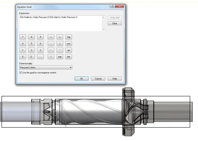
Figure 20. Outlet Boundary Condition of Average Static Pressure across the Surface of 909.98 mmHg . 28 Figure 21. Criteria Setting that Calculates dP for the Simulations ... 29
Figure 22. Residual Plot for Mass Flow Rate Criteria for 0.5 mmHg Residual Setting for the Average Inlet Pressure ... 30
Figure 23. Residual Plot for dP with 0.5mmHg Residual Setting at the Inlet ... 30
Figure 24. Mass Flow Rate Residual Plot for 0.25 mmHg Residual Setting at the Inlet ... 31
Figure 25. Residual Plot for dP with 0.25 mmHg Residual Setting at the Inlet ... 31
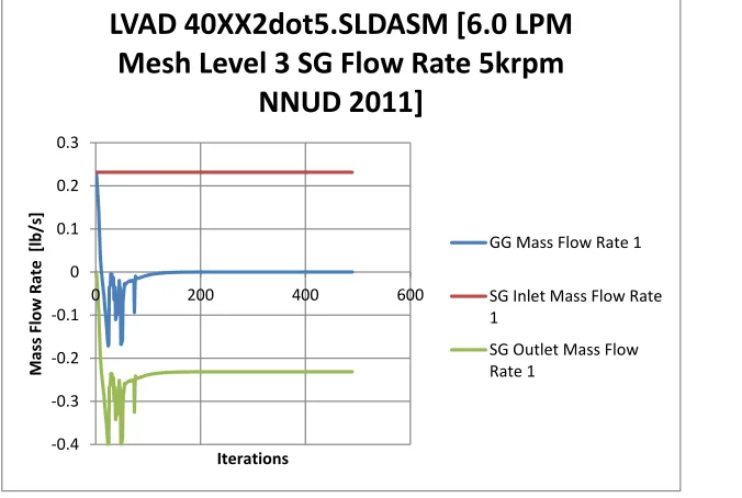
Figure 26. Example Residual plot of Mass Flow Rate for Finalized Settings ... 32
Figure 27. Example of Residual plot of dP for Finalized Simulation Settings ... 33
Figure 28. Bench Top Testing vs. CFD Simulation Flow Types Examined ... 34
Figure 29. Bench Top Testing Vs. CFD Simulation Flow Types for the Trimmed Impeller ... 35
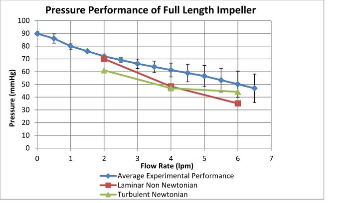
Figure 30. Pressure Performance for Finalized Setting of the Full Length Impeller ... 36
Figure 31. Trimmed Impeller ... 38
Figure 32. Comparison of Final CFD Settings to Bench Top Testing of Trimmed Length Impeller ... 38
Figure 33: Trend of Hemolysis as a Function of Length [38] ... 43
Figure 34-Shear Distribution Within Impeller Flow Region, Full Length Case on the left, Trimmed Case displayed on the right ... 45
Figure 36- Impeller 2.001 ... 51
Figure 37- Impeller 2.101 ... 52
Figure 38- Impeller 2.201(Original) ... 52
Figure 39-Impeller 2.301 ... 52
Figure 40-Impeller 2.401 ... 53
Figure 41-Impeller 2.501 ... 53
Figure 42. H-Q Curves of Design Iterations ... 54
Figure 43. Overall Pressure Output of Design Iterations ... 54
Figure 44. Computed NIH Values for Design Iterations ... 56
Figure 45. Percent Difference of NIH Values from Impeller 2.201 ... 56
Figure 46. Thrombosis Risk Percent Differences from 2.201 ... 57
Figure 47. Particle Study of 0.5 lpm Trimmed Impeller Simulation ... 61
Figure 48. Basic Mesh Setting Screen ... 69
Figure 49. Solid and Fluid Interfacing Setting Screen ... 69
Figure 50. Cell Refinement Setting Screen ... 70
Figure 51. Narrow Channel Setting Screen ... 70
Figure 52: Shear Distribution for the Second Forward Impeller Move ... 71
Figure 53: Flow Trajectory Paths for 0.5 Lpm ... 72
Figure 54: Flow Trajectory Paths for 2 Lpm ... 72
Figure 55: Flow Trajectory Paths for 4 Lpm ... 73
Figure 56: Flow Trajectory Paths for 5 Lpm ... 73
Figure 57: Flow Trajectory Paths for 6 Lpm ... 74
Figure 58: Flow Trajectory Paths for 0.5 Lpm ... 74
Figure 59: Flow Trajectory Paths for 2 Lpm ... 75
Figure 60: Flow Trajectory Paths for 4 Lpm ... 75
Figure 61: Flow Trajectory Paths for 5 Lpm ... 76
Figure 62: Flow Trajectory Paths for 6 Lpm ... 76
Figure 63: Flow Trajectory Paths for 0.5 Lpm ... 77
Figure 64: Flow Trajectory Paths for 2 Lpm ... 77
Figure 65: Flow Trajectory Paths for 4 Lpm ... 78
Figure 66: Flow Trajectory Paths for 5 Lpm ... 78
Figure 67: Flow Trajectory Paths for 6 Lpm ... 79
Figure 68: Flow Trajectory Paths for 0.5 Lpm ... 79
Figure 69: Flow Trajectory Paths for 2 Lpm ... 80
Figure 70: Flow Trajectory Paths for 4 Lpm ... 80
Figure 71: Flow Trajectory Paths for 5 Lpm ... 81
Figure 72: Flow Trajectory Paths for 6 Lpm ... 81
Figure 73; Flow Trajectory Paths for 0.5 Lpm ... 82
Figure 74: Flow Trajectory Paths for 2 Lpm ... 82
Figure 75: Flow Trajectory Paths for 4 Lpm ... 83
Figure 76: Flow Trajectory Paths for 5 Lpm ... 83
Figure 77: Flow Trajectory Paths for 6 Lpm ... 84
Figure 78: Flow Trajectory Paths for 0.5 Lpm ... 84
Table of Equations:
Equation 1 ... 7
Equation 2 ... 40
Equation 3 ... 40
Equation 4 ... 40
Equation 5 ... 40
Equation 6 ... 40
Equation 7 ... 40
Equation 8 ... 40
Equation 9 ... 40
Table of Tables:
Table 1. Original Spline Points ... 21
Table 2. Corrected Spline Points... 22
Table 3. SolidWorks Release Rerun ... 35
Table 4: Mesh Settings Applied ... 36
Table 5. Comparison of Simulation Efficiency and Accuracy ... 37
Table 6. Comparison Of Hemolysis Rates for Impeller Moves ... 44
Table 7-Changes in Inlet Angle for Designs Created ... 51
Table 8. Comparison Table for Design Iterations ... 55
Table 9. Hemolysis Grade and Percent Difference from 2.201 ... 57
Table 10. Thrombosis Grades and Percent Difference from 2.201 ... 58
List of Terms
Axial Blade Length- Length of the blade along the axis of rotation
Blade height- Distance normal to the hub surface to the top of the blade
Blade helix- The shape that the blade creates as it wraps around the hub from the leading edge to the trailing edge.
Blade length – Length of the blade if traced along the helix
Blade width- Distance between the opposing sides of the blade perpendicular to the hub surface
Diffuser- Component that redirects the rotational velocity components of flow into axial creating static pressure rise
Hemocompatibility- Measure of a devices ability to maintain healthy blood flow conditions, i.e. not causing hemolysis or thrombosis at an elevated level compared to normal biological conditions
Hemoglobin- Protein found in red blood cells that carries oxygen
Hemolysis- Rupture of red blood cells induced by shear stresses experienced in blood flow and to cell aging.
Impeller- Rotating component in a pump that imparts work upon the fluid
Inducer/stator- Component in a pump that directs flow into the impeller from the pump inlet
Inlet angle- Leading angle of the impeller’s blade helix, measured from the rotational axis
Left Ventricle Assist Device- A pump attached to the left ventricle of a weakened heart to aide in the pumping of the blood through the body
Normalized Index of Hemolysis- Universal and accepted measure of hemoglobin release by the scientific and medical community
NP-Hard- A problem is termed NP-Hard if the algorithm to solve it can be translated to solve any NP problem, (nondeterministic polynomial time) problem. Therefore NP-Hard means “at least as hard as any NP problem,” although in fact it may be even harder [1]
Outlet angle- Trailing angle of the impeller’s blade helix, measured from the rotational axis
Thrombosis- Clotting of blood and/or blood components, white thrombus are formed from platelets and red thrombus can be formed solely of red blood cells but can be a mixture of all blood components
1. Introduction:
1.1.Ventricular Assist Devices
The demand for medical devices increases daily as the medical industry tries to keep up
with maintaining patients’ health. One area of focus shared around the world is the development
of prosthetic replacements for key anatomy in the circulatory system. Due to challenges in
creating total artificial hearts, different approaches have cumulatively resulted in developing
pumps to aid the heart’s function. Pumps have been created to assist the right, left, and both
ventricles of the heart. In most cases of heart disease, where people are in need of a heart
transplant, a Left Ventricle Assist Device (LVAD) Figure 1 would negate the requirement for a
[image:18.612.180.311.356.539.2]donor to be found.
1.2.Background
1.2.1. The LVAD at RIT
Most current LVADs in use employ mechanical bearings, which damage the blood as
part of the blood flows through the bearings. The bearings themselves wear, causing limited
lifespan to the VAD. The LVAD in development at RIT uses magnetic forces to hold its
impeller in place and spin it. This LVAD is designed for long term to permanent installation for
those suffering from heart failure, thus freeing them of the dangerous wait for suitable a donor.
For several years this axial device has been in its many stages of development. The size has been
scaled down by new case design, new magnetics, and shortening the axial legnth of the original
pump. Now, improvements in impeller blade design are one of the few areas less explored. The
LVAD has been implemented in animal trials to produce data that will be used in conjunction
with other preliminary performance data from lab experiments to set the baseline for
improvement. Like many other VADs, this device is a rotary pump, making the interaction
between the impeller blades and the blood the main area of focus. The key parameters driving
the optimization of this pump are flow and pressure output, as well as the levels of thrombosis
and hemolysis through the pump. The goal of this study is to create and implement a strategy to
improve the impeller design of RIT’s axial VAD, with objectives of lowering the risk of
hemolysis and thrombosis, while increasing head and flow output.
The current version of the system is the LVAD-40XX which uses the Imp
2500_421_V3b as the impeller model and is shown in Figure 2. This version of the system has
been tested through both bench top experiments and a 28 day trial in a calf. Below are charts for
the H-Q curve and hemolysis performance in terms of free hemoglobin level in the blood stream.
At present there is no way to assess thrombosis, except by checking for clots after animal trials.
With less than ten animal trials completed information on thrombosis formation is limited.
Pressure and hemolysis performances are displayed in Figure 3 and Figure 4 are fromthe excel
files “Pumps Performance Curve in Blood between P2 and P3” and “data sheet of hemolysis
between two pumps”, respectively. The pressure data was compiled from two separate trials
completed on different dates with fresh blood from the same source. The average of the two data
Figure 2. LVAD Assembly for Simulation (Only Fluid Interfacing Components)
Figure 3. Pressure v. Flow Rate of Bovine Blood in Laboratory Testing of LVAD-40XX[3] 0
20 40 60 80 100
0 1 2 3 4 5 6 7
Pres
sure
(mmHg)
Flow Rate (lpm)
Average Performance (9/11/09 & 5/12/09)
Figure 4. fHb Vs. Time of Fresh Bovine Lab Trial of LVAD-40XX[4]
1.2.2. Biological Demands
As the left side of the heart is responsible for transporting oxygenated blood to the body
which demands higher pressure output, only the function of the left side of the heart will be
discussed to define cardiac demands. Normal ventricular performance provides the body with a
flow rate of 5 liters per minute at the normal maximum of 120 mmHg of created pressure. Due
to the nature of the hearts pumping process, the flow is pulsatile. A cardiac cycle consists of two
phases starting with diastole then systole. Diastole begins as the left atrium contracts causing the
mitral valve to open and allow oxegenated blood to flow from the atria into the left ventricle.
Systole begins after the mitral valve closes and the left ventricle contracts to create pressure to
open the aortic valve and eject oxygenated blood into the aorta. The two-phase cycle then
repeats itself indefinitely. Figure 5 represents the cardiac cycle graphically. Each phase is
indicated as are all major valve openings and closings. The atrial, ventricular, and aortic
pressure are graphed along the same axis as the ventricular volume to when the ventricle begins
to contract the pressure rises in the ventricle and aorta.
y = 0.0731x R² = 0.9705 y = 0.071x R² = 0.8632 y = 0.0719x
R² = 0.9554
0 2 4 6 8 10 12 14
0 50 100 150 200
fHb (mg/dL)
Time (mins)
9/10 Results Rig 3 at 5,6 and 3 LPM
Figure 5. Typical Cardiac Cycle Graph for Pressure and Ventricular Volume [5]
As a heart becomes weakened, the pressure peak and ejection volume lessen. In severe
cases the heart can only produce a mere fraction of the normal outputs,where an LVAD needs to
be able to provide near complete left ventricular output to be able to support such patients[2]. An
LVAD attached to the left ventricle also operates cyclicly in terms of pressure and flow
generated. As diastole begins and the vetricle is filled, an inlet canula attached to the bottom of
the ventricle directs some of the flow into the assist pump’s entrance. The inlet flow to the
LVAD device is approximated at 0.5 liters per minute during this phase for this project but can
vary greatly patient to patient. As systole begins, the ventricle contracts and simultaneously
ejects blood both into the aorta and the inlet of the LVAD. At this point the flow rate is
approximated to be six liters per minute for this experiement. The flow rate during this phase
varies person to person, and can range up to 10-12 liters per minute. The low flow rates during
diastole allow the LVAD to create a high pressure change that lowers as the flow rate increases.
With this functionality the LVAD matches the demands of the normal cardiac cycle. With these
needs to keep patients alive, a LVAD device is given the operation range of zero to six liters per
1.2.3. Pump Design Theory
A diagram of the pumps fluid interfacing components highlighted and named will be
reviewed to better understand the subject material to follow in this section. The fluid flows
through the pump from left to right as pictured in Figure 6. The working fluid is directed into the
impeller, highlighted by red, through the stator, or inducer, which is highlighted in yellow. The
impeller imparts energy into the fluid in the form of kinetic energy in the form of axial and
rotational velocities. The pressure is then recovered from the fluid flow by converting the
rotational velocities into pressure by straightening the flow. This energy conversion takes place
as the fluid leaves the impeller and enters the diffuser which is highlighted in orange.
Figure 6: Pump Assembly with Stator Highlighted in yellow, Impeller Highlighted in red, and Diffuser Highlighted in orange
Conventional pump design theory looks mainly at the fluid and solid body interaction at
the inlet and outlet to derive fluid mechanical performance. At the inlet the interaction between
the stator angle and leading blade angle are calculated to approximate inlet performance and
limits. Pump dynamics can also be approximated at the outlet via the trailing blade angle and the
diffuser inlet angle. These types of calculations use velocity triangles to evaluate changes in
flow direction and speed [6]. From this information, pressure changes can be approximated.
Figure 7 shows an example of velocity triangle diagrams for an axial compressor stage and the
pressure gain across the stage, where U is the translational speed due to rotation; cy1 is the
measure of the stator inlet angle from the axial direction; and cy2 is the measure of the inlet blade
approximated as long as the density of the fluid is also known, as shown in Equation 1, the
pressure ratio for the stage can be calculated. These calculations are used to make rough
estimations of the pump dynamics and are more useful to better understand the general effects of
design changes, rather than trying to calculate true performance.
Figure 7. Velocity Triangle Diagrams for an Axial Compressor Stage and the Pressure Gain Across the Stage[6]
∆𝒑
𝝆 = 𝑼(𝑪𝒚𝟐− 𝑪𝒚𝟏)
Equation 1
The most common method to display pump performance is by a head-flow (H-Q) curve.
This type of graph plots the pressure head generated at the flow rate for a specific operating
speed of the pump. The graph typically displays pressure head on the y-axis as a function of
volumetric flow rate along the x-axis. As seen in Figure 8, the resulting curve displays the
relationship of pressure generated in comparison to flow rate. As flow rate increases, the
pressure added to the fluid drops if rotational speed is kept constant. These curves are most often
used to choose pumps based upon flow rate head requirements. In the case of the LVAD for this
experiment, flow rates vary from zero liters per minute to six liters per minute, but can truly vary
To make direct comparison possible between all designs, the operating speed was set to
5,000 rpm and kept constant. The pressure head flow curves for the LVAD at RIT can be
displayed in one graph to allow for quick visual comparisons. The area under these curves can
be used for comparison purposes as an absolute measure of pressure generation performance
over the operating range. Fitting equations to the curves will allow for numerical comparisons
by using the integrals of the equations over the ranges tested in Computational Fluid Dynamic
(CFD) simulations.
Figure 8. Sample H-Q Curve [6]
1.2.4. Blood Pump Design Strategy
There are many separate efforts across the globe working toward the best solution to
ventricular support. Several of these ventricle assist devices have completed an optimization
effort of differing methods [7-11]. The project lead by Sorguven devised a method used to
attempt to optimize the design of an axial LVAD’s impeller, which involved creating random
then made and assessed [8]. Sorguven cites the loop shown in Figure 9 depicts that an individual
model was generated, tested, and then improved upon. In the experiment Sorguven skips the
optimization module that is to determine the new design. Sorgeven lacked full analysis of each
design before the next design was created. Improving upon Sorgeven’s methods, the design
strategy for this project created impellers one at a time, assessed the three performance
parameters (head generation at a given flow rate, hemolysis rate, and thrombosis risk), and then a
design alteration was made to create the next impeller to be tested. This was repeated until the
local (within set design constraints) optimal design is created. Of the projects encountered
through research, no others have set forth to truly find the true optimal impeller design within the
current system design restraints [7-11]. Instead, most studies attempt to correct known issues
within the flow field with only a few iterations [7, 10, 11]. Some projects used intuitive analysis
for each iteration to base design changes for the next model [7, 9]. Assessment of the designs
was limited to visual inspection of simulation [7], or flow visualization results from high speed
video of particles traveling through the pump tested[9]. Design improvements were based upon
basic pump design theory and an in-depth understanding of the flow phenomena within the
pump. The work completed within this project involved an objective and quantitative
assessment of each design iteration that guided where to continue within the available design
space.
The difference of this study compared to others is that both a qualitative and quantitative
assessment of the simulation results was completed before design alterations were made. Not
only was there a visual inspection the particles traces through the pump form CFD results, but
also data was output from the mesh to provide shear and velocity data.
SolidWorks Flow was used to run simulations of the VAD to provide pressure, velocity,
and shear (velocity and shear values used to estimate thrombosis risk and hemolysis rates
respectively) values at tested flow rates. With the data created from simulations calculations and
comparisons were made to assess overall performance.
1.2.5. CFD Modeling of Blood Pumps
To save money and time Computational Fluid Dynamics has been employed by many
design efforts to model the flow through the blood pump in development [12, 13]. Due to
advances in both computing capability and CFD software, complicated flow paths such as the
one through a turbomachine can be modeled accurately. It has been noted from experiments that
blood will maintain a constant viscosity when exposed to shear rates greater than 100 s-1. This allows for a Newtonian blood model to be created in any CFD programs data bank, setting the
density at 1050 kg/m3 and the viscosity to 0.0035 Pa×s [12]. CFD packages also offer options of what type of flow is to be modeled. The flow through a pump isn’t laminar due primarily to the
small gaps that the fluid travels through and also the rotational input of the impeller. Both of
these cause a large velocity differential and a generally large rise in Reynold’s Number. Popular
options for modeling the turbulence are the k-ϵ and k-ω turbulence models. The k-ϵ model is
better suited to fully turbulent flow analysis, where Reynold’s numbers are well past the
turbulent transition [14]. The k-ω is designed to provide accurate modeling for transitional flows,
as well as turbulent flows, and has displayed accuracy across both laminar and turbulent flow
regions. The k-ω turbulence model is gaining popularity due to its accuracy in the boundary
layer, which grows off the wall surfaces [13, 14]. It has been used with success by other VAD
design teams[14]. Meshing is arguably the most crucial step in flow modeling and is critical to
acquire accurate solutions upon convergence. Each pump’s demands are different, so the general
approach to meshing blood pumps is refinement in the blade gap region, or any narrow gap, and
accuracy study to finalize mesh geometry. To finalize model settings, appropriate boundary
conditions must be applied. The following settings described are general for the frozen rotor
style of simulation. All solid surfaces are given the real wall condition, with the surface
associated with the impeller given a steady rotational speed and then housing walls given the
stationary condition. Also, a rotating zone must be indicated to define what section of the
computational domain is rotating. The inlet boundary condition is set to a steady volumetric
flow rate. The outlet is set to constant pressure. Convergence criteria are commonly
conservation of mass (COM) and pressure change across the pump (∆P), but others can be added
to meet the demands of the design effort. When simulations are complete many software options
allow for the export of the performance data such as pressure head and shear rates for each mesh
element in the computational domain. Many aspects of performance are available to output in
many forms, data dumps to excel or text files are two popular choices. Contour charts, path-line
studies, particle traces, and others are used to provide useful information about the flow stream
through the pump. With this data output from CFD simulations, design performance can be
measured without bench top experimentation [14, 15].
1.2.6. Hemolysis
When red blood cells are exposed to high shear rates they risk suffering hemolysis, defined as
the rupture of a red blood cell where hemoglobin is released [16]. In lab experiments hemolysis
is measured by recording the rise in free hemoglobin in the plasma [16-22]. In simulation
hemolysis is estimated by a relationship including the magnitude of shear stress and exposure
time to that stress [11, 12, 14, 15, 23-25]. Two types of shear stress are created in the flow path
of an LVAD. Viscous stresses can be induced in both laminar and turbulent flows, while
Reynolds stresses exist in turbulent flows only. As of current, the more proven damage models
utilize laminar shear stress. This coincides with the fact that shear rate data was only available in
laminar simulations. The amount of hemolysis that a VAD creates is considerably important and
is a large contributor to defining the overall performance of a VAD.
1.2.7. Thrombosis
Thrombosis is sometimes considered the more dangerous of the two types of blood damage as it
of shear, chemical triggers, and areas of stagnation [7, 9, 10, 26, 27]. What makes thrombosis
more difficult to predict than hemolysis is that no definitive relation has been developed between
fluid dynamics and thrombosis formation. Known risks are high shear rates, low shear rates,
recirculation, stagnation points, material composition, and surface finish. Surface finish and
material choice at this point are not of high concern. Medical approved titanium alloys have
remained the material of choice for impellers, though there has emerged injection moldable
ceramics that have the potential to replace titanium [28]. High shear rates cause hemolysis,
which releases the contents of red blood cells and can lead to platelet activation, thus forming
clots [27]. Low shear rates should be avoided, since they allow platelets to stick to cell walls.
Areas of stagnation and recirculation are risk points as flow velocities approach and sometimes
reach zero. Stagnation points lead to clotting as seen in some early versions of centrifugal
pumps where some flow must pass behind the impeller [10, 11]. Establishing the safe minimal
flow velocity and channel width have been found to deter thrombosis formation. Recirculation
points by theory elevate the risk of thrombosis due to stagnation points at their centers and low
shear rates, although no direct relation has been linked to thrombosis formations. Recirculation
flow patterns have been seen in both CFD simulations and other flow visualization trials of
various pumps, yet no significant thrombosis has occurred in the pumps tested when they
reached whole blood or animal trials [9, 28-30]. Most thrombosis seen is at the fittings to the
inlet and outlet to the pumps that use barbed fittings. Only a small number exhibited clots within
the pump and it is not always clear if the clot formed elsewhere in the test loop or animal. At
this point the only true way to assess thrombosis is through whole blood or animal tests. In
whole blood flow loop tests the pump and system are inspected for clots. In animal tests, the
1.2.8. Design Concerns
Figure 10: Impeller with inlet angle indicated in Red and Initial and Terminal Helix Points in Yellow
In Figure 10 several key features to the design of the impeller and displayed. The blade
helix is the series of cylindrical coordinates that defines the blade shape. The inlet angle is the
angle the helix creates where it intersects the axis of rotation at the inlet side of the impeller. The
wrap angle is the total measure of rotation the helix from the leading edge to the trailing edge.
Figure 11. Enlarged View of Entry Region to the Pump with Inducer Highlighted
One area of concern for performance in an axial pump is the entrance region immediately
before the inducer and the first third of the impeller, as shown in Figure 11. The region
immediately upstream of the impeller blades and stator holds a high risk for recirculation, which
leads to possible stagnation points and can cause thrombosis. This section has the risk of
cavitation and high shear between the wall and impeller blade. The entry region to any pump
into the fluid is completed by the first half of the length of the blade. This kinetic energy is then
converted into pressure by converting rotational velocities to pressure in the diffuser. The
interaction with the diffuser and the impeller dictates pressure rise making this region the other
area of concern for performance. The gap between the wall and impeller throughout the pump
has the greatest potential to produce the highest shear rates. The gap is only 0.010” and holds the
largest velocity gradient due to the rotational speed of the blade, which is 5000rpm for all
simulations and no slip at the housing wall.
1.2.9. Optimization Theory
Design optimization is the process where a device, or component, is redesigned to best
meet performance demands within set design constraints. The process of creating iterative
designs to find the optimal design is the design search. Methods to complete the optimal search
vary depending on the complexity of the design and performance criteria among other reasons.
Each design aspect that can be varied adds to the design space available to search. Design search
methods are often picked due to the size of the open design space. Search method selection is
also driven by how many performance parameters are taken into consideration. For very simple
design searches, where one design parameter is available, a simple difference method can be
used. The difference method can be employed in multiple parameter searches but more effective
schemes exist to handle the larger design space. For a one parameter search the design would
vary in one direction within the design variable until performance drops. Design alteration will
then resume but headed in the opposite direction. The search continues again until performance
drops. At that point the design that performs best is considered the optimal design within the set
design space. Mathematically optimal searches find the minima, they look for where change in
performance approaches zero while performance is at a maximum [31, 32]. The design process
can be automated using numerical approaches. As design spaces grow, numerical methods can
be employed to conduct design searches to handle the larger design space [31, 32]. As numerical
methods require the mathematical parameterization of both the performance and design variables
into equations to be assessed to locate the minima, or maxima, the difficulty of setting up these
searches grows with design complexity and the number of performance parameters involved.
With extremely difficult design problems it has been noted that design searches can be conducted
more efficiently by an engineer with knowledge in the specific area of design concern [33]. The
search. Each project shapes the methods employed to best fit the design problem that needs to be
addressed.
Optimal design searches are defined not only by the performance of the device to be
improved but also by the constraints on the development of the project. The performance criteria
of a blood pump are: 1) pressure output over the operating range of flow rates, 2) level of
hemolysis, and 3) risk of thrombosis. Having multiple design and performance parameters
expands the design search, as first a definition to optimal performance has to be created. Each
performance parameter must first be ranked for importance and assigned a weight for the grading
scheme to be used to assess the iterations. Having multiple design parameters expands the
design space exponentially in terms of each design parameter. Numerical methods of optimal
design are often believed to provide the most accurate and rapid results for most optimal
searches. With multiple performance and design parameters, the problem becomes exponentially
more demanding in terms of computing and pre- and post-processing demands. To complete an
automated parametric study the impeller design would have to be separated into variables that
can be altered easily. The helix does not allow for one step design changes, though the helix can
be modified by the control of a single variable, the blade itself is then modeled through a series
of operations. This does not allow the blades to be directly modified within SolidWorks via one
variable. The complexity of the design was another factor that lead to the exploration of an
alternate method to numerical methods for optimization [31].
When dealing with complex systems the common route is to model the system and setup
an automated mathematical scheme to define the design performance and alteration [32]. This
type of optimization works for systems with linear relations to the design parameters being
altered. The relationship between some of the design parameters of this impeller and the
performance is undoubtedly non-linear. This makes the system extremely hard to parameterize
between having linear relations and trying to model non-linear relations as linear. Overall
performance is dependent on all of the design parameters and hence is non-linear. Design
problems involving even two non-linear relations most often fall into the terms of NP-Hard. The
issue with using an automated design search is that this design problem most likely falls into the
classification of NP-Hard. When multiple parameters are open to design changes and there is
nature of optimizing the impeller of the LVAD-40XX most likely lays in the realm of NP-Hard
where heuristic methods prove effective in design problems of this classification [33]. From
short research on the basics of Design of Experiments a general approach formulated to meet the
design tasks. The impeller blade design involved many variables, each of which are interrelated
in terms of performance. These types of systems are usually accessed better with a factorial
experiment to gain a better understanding of each variables effect on the systems performance
[34]. In the case of the impeller design that would mean examining the effect of several design
changes to each variable to be tested. After these initial trials for parameter performance effect a
refined design path can be made from the information gained.
1.3.Motivation
Early rotational blood pumps exhibited high level thrombosis due to bearings obstructing
flow through these devices. Now as designs shift to magnetically levitated devices the challenge
is ensuring direct flow through the pump to greatly reduce the risk of clotting. The challenge
then becomes to eliminate stagnation points in the pump and provide enough shear stress to
“wash” all surfaces, but not lyse the cells. Improving the pressure output while reducing the
hemolysis at the same operation speed may lead to the pump being able to run at a lower speed
to attain necessary pressure output. This would reduce the risk of hemolysis directly as shear
stresses are mainly created due to the rotational speed of the impeller. In the future this may
even lead to a scaling down of even the hub diameter, which could lead to a whole new round of
miniaturization of case and internal electronics.
The aim of this study is to implement and test a design strategy to develop optimized
impeller geometry. The most important component in any rotary VAD is the impeller, as it
transfers energy into the blood to provide mass flow and increase pressure. Due to this fact,
most of the efforts in VAD design are focused on design refinement of the impeller. Impeller
performance is assessed by head and flow output along with blood shear rates and velocities that
will be used to estimate blood damage. Though other design efforts have been completed to
improve VAD impeller design, few to none assess design performance both numerically and
visually before generating the next iteration in the design space. The design path of this project
was directly dictated by the full assessment of each iterative design to indicate parameters for
2. Methods
2.1.General Approach
The initial proposed designs (Proposed Design Path) were modeled in SolidWorks.
Design iterations were tested in SolidWorks FLOW to model pump operation (CFD Simulation).
Data was recorded across the entire computational domain for velocity and shear rate, along with
the cells’ x, y, and z location, size and volume. The data was output into a text file and the values
were accessed by a MATLAB code to evaluate the risk of thrombosis and the level of hemolysis
(Individual Performance Grading). The pressure performance was calculated using MS Excel to
fit curves to the pressure output at each tested flow rate (Individual Performance Grading). From
results of the MATLAB code, the design was graded along with pressure data gathered in Excel
using grading matrices to get an overall grade (Overall Grading Matrices). From that grade we
gained an understanding of what areas of performance that were in need of an increase. The new
design was proposed to correct the deficiencies of the previous iterations, or increase the gains
made if no general deficiencies were seen (Design Alteration). This cycle was repeated until the
performance dropped in all design directions tested. These steps are highlighted in Figure
CFD
Simulation
Individual
Performance
Grading
Design
Alteration
Overall Grading Matrice
Proposed
Design Path
Optimal
Design
Strategy
Figure 12. Design and Testing Loop
2.2.Difference Method for Optimal Search
A simple difference method was employed to find the maxima of one design variable.
The maxima for this design search was the highest overall grade over the three performance
parameters. The open design parameter was varied incrementally in one direction to begin the
search. Performance was monitored as iterations moved from the initial design. Design
variation continued in the initial direction until performance dropped. Due to the nature of the
helix, it is highly unlikely that performance would rise overall within the set operating range if
performance dropped in the first design direction, the design variation returned to the initial
design, and variation from the initial design then continued in the opposite direction from the
first explored. When performance dropped off in the other design direction, iterations were
ceased and the local maxima of each design direction was compared to find the global maximum.
The optimal search for the LVAD 40XX consisted of varying the helix equation to
modify the helix shape. Performance was measured in terms of pressure generated, hemolysis
induced, and risk of thrombosis formation. The three performance terms were compiled into a
final performance grade to serve as an absolute measure of performance. The helix was first
modified to lower wrap angles until performance dropped. Then, the helix wrap angle was
increased until performance dropped in the opposite direction. Jumps forward in either direction
were not necessary because modifying the helix in either direction would cause cavitation.
2.3.Proposed Design Path
The design constraints were primarily based on the fact that all designed impellers had to
fit within the current pump package. This set the maximum diameter, overall length of the hub,
and hub inlet and outlet angles. These constraints still allowed for changes to blade length,
height, width, inlet and outlet blade angles, and helix shape. In the past the blade-hub interface
created acute angles, as shown in Figure 13, which were not allowed to be worked into impeller
designs due to manufacturing restraints as mentioned in the R-005 Machinability Report [35].
Previous simulations had proven the acute angles were not necessary for pump performance. A
new design was created so that the angles perpendicular to the hub surface were instead
perpendicular to the axis of rotation. With these geometric constraints set, pump design and
fluid dynamic theory was applied to correct the flow patterns that posed as risks for blood
Figure 13. Compound Blade Angle with hub Surface Creates Acute Angle[35]
To keep the current magnetic assembly the hub geometry was not modified. Available
design parameters left open to modify were; the blade helix (inlet and outlet blade angle and
wrap angle were adjusted through this), blade height, width, and length. To allow for a timely
design search the design parameters were reviewed to assess parameter effects on the
performance of the system to choose one to allow for a simple optimal design search to provide a
proof of concept. Blade height was a very critical and sensitive design variable. Blade height
was ruled out due to two concerns. If the blade height was increased, then the risk of crash
would greatly rise as the gap between the impeller blade and cannula wall is only 0.010”. Also
the risk of hemolysis generally rises with tighter blade clearance due to extreme shear rates
created in the gap. However, lowering the blade height detracts from pressure performance due
to the drop in surface area available to transfer energy into the blood passing through the pump.
Due to issues that occurred while testing a lower blade length, blade length was also kept
constant. These issues are reviewed later in this text. The ability to modify three parameters at
once by modifying the blade helix caused it to be the most important variable to investigate.
Inlet angle is largely related to the suction head created to pull fluid into a pump. Wrap angle
controls the overall blade length which effects the total bladed area able to transfer energy into
the flow stream. The outlet angle is greatly responsible for pressure recovery in relation to the
flow direction entering the diffuser. These reasons ruled out the blade width, as such it was kept
constant. The ability to modify all three of these design parameters with one variable allowed for
the possibility to greatly effect performance with small iteration steps. To define the helix
define the original geometry of the blade helix. This helix was the product many tests and
calculations and was believed to be the optimal for the original LVAD at RIT. The original helix
points were provided from LVADR2 2.3 Spline Points-RevB.xls to allow for a regression to be
completed providing the original helix point equation. The helix was designed in cylindrical
coordinates originally and converted to Cartesian coordinates. The “r” value sets the radial
length from the axis of rotation. Θ is the value of the angle of rotation from the origin, and Z is
the value of the displacement along the axis of rotation. Shown in the Table 1 below are the
original helix points.
Original Blade Spline
Cartesian Points Cylindrical Points
x y Z R z
mm mm Mm Mm radians mm
-0.830 3.110 3.410 3.219 1.832 3.410
-1.740 3.020 3.890 3.485 2.094 3.890
-2.700 2.710 4.540 3.825 2.354 4.540
-3.700 2.150 5.370 4.279 2.615 5.370
-4.620 1.260 6.320 4.789 2.875 6.320
-5.420 0.020 7.500 5.420 3.138 7.500
-5.990 -1.570 8.920 6.192 3.398 8.920
-6.180 -3.520 10.620 7.112 3.659 10.620
-5.830 -5.760 12.640 8.196 3.921 12.640
-4.150 -7.070 15.020 8.198 4.182 15.020
-2.180 -7.900 17.780 8.195 4.443 17.780
-0.070 -8.200 20.920 8.200 4.704 20.920
2.050 -7.940 24.270 8.200 -1.318 24.270
4.030 -7.140 27.940 8.199 -1.057 27.940
5.740 -5.860 31.940 8.203 -0.796 31.940
7.050 -4.180 36.370 8.196 -0.535 36.370
7.890 -2.220 41.310 8.196 -0.274 41.310
8.200 -0.100 46.970 8.201 -0.012 46.970
7.950 2.020 53.640 8.203 0.249 53.640
7.160 4.000 60.640 8.202 0.509 60.640
Table 1. Original Spline Points
There was a shift in theta values from the original blade points. The angular position
could not be accurately fit to one equation from the way the original points were expressed.
Angular position was listed as increasing along the axis of the hub until it achieved the value of
24.270 mm, where it was then expressed in negative terms. This required a piece wise log fit to
positive increasing order. With this format, one equation was regressed to provide the baseline
for modification. Also the radius of the spline points was set to a nominal 8.200 mm along the
length of the impeller where the hub radius is constant. Shown in Table 2 is the spline points
along the hub expressed in both Cartesian and cylindrical forms, along with the cylindrical form
of the extended points. Following the list of points is the plot of the log natural fit of the spline
points compared to the actual points themselves shown in Figure 14.
Blade Spline (referenced from hub triangle / axis intersection)
Cartesian Points Cylindrical Points Extended Points
x y z r z Corrected Radius r z
mm mm mm mm Radians mm mm mm radian mm
-0.830 3.110 7.580 3.219 1.832 7.580 4.376 6.974 1.832 6.080
-1.740 3.020 8.060 3.485 2.094 8.060 4.653 7.252 2.094 6.560
-2.700 2.710 8.710 3.825 2.354 8.710 5.029 7.627 2.354 7.210
-3.700 2.150 9.540 4.279 2.615 9.540 5.508 8.106 2.615 8.040
-4.620 1.260 10.490 4.789 2.875 10.490 6.056 8.654 2.875 8.990
-5.420 0.020 11.670 5.420 3.138 11.670 6.738 9.336 3.138 10.170
-5.990 -1.570 13.090 6.192 3.398 13.090 7.560 10.300 3.398 12.381
-6.180 -3.520 14.790 7.112 3.659 14.790 8.140 10.700 3.659 14.572
-5.830 -5.760 16.810 8.196 3.921 16.810 8.200 11.200 3.921 16.810
-4.150 -7.070 19.190 8.198 4.182 19.190 8.200 11.200 4.182 19.190
-2.180 -7.900 21.950 8.195 4.443 21.950 8.200 11.200 4.443 21.950
-0.070 -8.200 25.090 8.200 4.704 25.090 8.200 11.200 4.704 25.090
2.050 -7.940 28.440 8.200 4.965 28.440 8.200 11.200 4.965 28.440
4.030 -7.140 32.110 8.199 5.226 32.110 8.200 11.200 5.226 32.110
5.740 -5.860 36.110 8.203 5.487 36.110 8.200 11.200 5.487 36.110
7.050 -4.180 40.540 8.196 5.748 40.540 8.200 11.200 5.748 40.540
7.890 -2.220 45.480 8.196 6.009 45.480 8.200 11.200 6.009 45.480
8.200 -0.100 51.140 8.201 6.271 51.140 8.200 11.200 6.271 51.140
7.950 2.020 57.810 8.203 6.532 57.810 8.200 11.200 6.532 57.810
7.160 4.000 64.810 8.202 6.793 64.810 8.200 11.200 6.793 64.810
Figure 14. Logarithmic Fit of Original Spline Points
The equation from the curve fit of the original spline point has a leading coefficient of
2.201, whose value set the name for each design. Hence the original impeller became impeller
2.201. When the leading coefficient was changed, the new value used in the helix equation was
used to name the new design. Using the value of the coefficient for each new helix to name the
design made it easy to track design changes and understand the difference of each iteration.
Using the leading coefficient of the helix equation as the name also helped to relate the change
seen in the physical part from the change made to the equation. The helix was due to be
modified in both directions during the search, so two test designs were made by iterating one
step in each directions. These two test designs were created to ensure that no difficulties would
arise when new blade helixes were created from modifying the helix equation. The designs are
2.301 and 2.101, based on the initial helix coefficient 2.201 that was varied by 0.1 in both
directions to test performance sensitivity and its effect on the helix shape. Figure 15 and Figure
16 show the difference in the first two designs. The inlet blade angle is defined as the angle
created by the leading edge of the blade and an intersecting line perpendicular to the axis of
rotation. As the coefficient was lowered the blade angle at the inlet increased and the opposite
occurred when the coefficient was raised, which can be seen when comparing the two impellers. y = 2.201ln(x) - 2.3778
R² = 0.9984
0.000 1.000 2.000 3.000 4.000 5.000 6.000 7.000 8.000 9.000
0.000 20.000 40.000 60.000 80.000 100.000 120.000
Angu
lar Posito
n
(radi
ans)
Axial Position (mm)
Spline Point Vs. Natural Log Regression
Figure 15. Impeller 2.101-Note that the Inlet Blade Angle is Larger than the Inlet Blade Angle of Impeller 2.301
Figure 16. Impeller 2.301
2.4.Model Generation
SolidWorks was used as the design package for creating the models of the new impeller
designs. This software package has been used for the lifespan of the project and met all of the
model was recreated with a more efficient modeling scheme to allow for facile geometry
changes, making iterations easily accomplished.
2.5.CFD Simulation
2.5.1. CFD Overview
The FLOW CFD package is an add-on for SolidWorks and was used for the all CFD
simulations for the new impeller designs. Applying simulation settings in FLOW was easier due
to work involved with applying boundary conditions to new geometries that were tested. Since
the models were created within SolidWorks, they didn’t have to be uploaded into a gridding
utility to have a mesh manually created for each geometry. Time was saved as each impeller
design needed only to be loaded into the simulation assembly and the mesh settings would
automatically generate a mesh. The preliminary simulations began running on a computer with
an Intel Core 2 6700 @ 2.66GHz and 8GB of ram of the same bus speed. Several computers in
the CFD Laboratory (Gleason 2271) were enlisted to complete the simulations during the final
stages of preliminary analysis and remained the computing stations for the remainder of the
project. All computers used were identical both in terms of software and hardware. The units
feature an Intel® Xeon® X3440 @ 2.6 GHz with 4.0 Gb of ram of the same bus speed. The
first accurate simulation result had a running time of twenty hours. Studies to determine
repeatability and accuracy at several operating points had been run to find the necessary settings
to achieve an accurate and repeatable simulation when compared to bench top test results. Once
a simulation had completed, it was easy to view and output the necessary results to assess the
specific iteration’s performance. The data needed for the hemolysis and thrombosis analysis was
output from the mesh into a text file. A MATLAB code was then used to assess the hemolysis
and thrombosis. The flow rates tested were 0.5, 2, 4, 5, and 6 liters per minute with the impeller
rotation of 5000 rpm.
2.5.2. Testing and Validation of CFD Simulation
2.5.2.1. General Settings:
A simulation can only provide valid information to use if accurate and repeatable results
are gained. To determine the accuracy of the solver and simulation settings used in FLOW, a
within the assembly that enveloped the impeller and inner walls of the cannula body. This part
served to indicate the region in which a moving mesh was necessary. There were several
boundary conditions necessary to set up a simulation of the pump. At the inlet of the pump there
was volume flow boundary condition (Figure 17) that was applied uniformly across the cross
section of the inlet cannula. On the exterior surfaces of the impeller a rotor boundary condition
(Figure 18) was applied to indicate a real wall (no-slip) condition as well as to indicate the body
within the rotating region that was spinning. The stationary walls of the cannula body were
given a stator boundary condition (Figure 19) also with a real wall condition specified. At the
outlet of the pump a pressure boundary condition (Figure 20) was set across the cross section of
the outlet cannula. These settings allowed for a simulation to run and converge but was not
repeatable.
Figure 18. Impeller Outer Surface Indicated with Rotational Boundary Condition
Figure 20. Outlet Boundary Condition of Average Static Pressure across the Surface of 909.98 mmHg
There are many aspects of the simulation that have been examined to ensure that a
converged result was achieved. A check for mass conservation through the pump was achieved
by checking both the mass and volume flow rates at the exit and entrance. The static and total
pressures were also examined at the entrance and exit surfaces. The last criteria to monitor was
the pressure differential created across the pump. The pressure differential (dP) was measured
by monitoring the difference of the average static pressure at the inlet from the average static
pressure at the outlet. Equation Goal 1 exemplifies the criteria setting that calculates dP for the
simulations, as shown in Figure 21. Convergence was measured by the change of the values of
these criteria between iterations. As the change dropped to near zero, the standard being a value
Figure 21. Criteria Setting that Calculates dP for the Simulations
The preliminary simulations could compute results accurately, but proved poor in terms
of repeatability. This was due to the solution oscillating from not reaching convergence before
the simulation iterations stopped When the residual plots, Figure 22 and Figure 23
,
for thesimulation were examined it was noticed that the pressure differential (dP) was the culprit having
caused poor repeatability. FLOW was set up to automatically assign residual size as calculations
were completed. To find the correct residual setting a series of simulations were completed with
various residual sizes that were set manually to the inlet pressure, as the outlet pressure was set
as a boundary condition. After the study was completed it was deemed that a setting of
0.25mmHg for the pressure residual at the inlet was sufficient, as seen in Figure 24 and Figure
25. This setting displayed convergence in terms of mass flow rate, while keeping simulations to
a reasonable 6-8 hours for most flow points. The 0.5L flow point could take days to converge,
but any coarser of a setting would result in a drop of accuracy and repeatability due to a slight
drop in convergence.
Figure 22. Residual Plot for Mass Flow Rate Criteria for 0.5 mmHg Residual Setting for the Average Inlet Pressure
Figure 23. Residual Plot for dP with 0.5mmHg Residual Setting at the Inlet -0.06
-0.01 0.04 0.09
0 200 400 600 800
Mas s Fl ow Rat e [lb /s] Iterations
LVAD 40XX.SLDASM [2.0 LPM Mesh
Level 3 SG Flow Rate 5krpm lam
0.5mmHg]
GG Mass Flow Rate 1
50 55 60 65 70 75 80
0 200 400 600 800
Equ at ion_ Goa l_ 1 [mm Hg] Iterations
LVAD 40XX.SLDASM [2.0 LPM Mesh Level 3 SG Flow
Rate 5krpm lam 0.5mmHg
]
[image:47.612.52.413.377.590.2]Figure 24. Mass Flow Rate Residual Plot for 0.25 mmHg Residual Setting at the Inlet
Figure 25. Residual Plot for dP with 0.25 mmHg Residual Setting at the Inlet -0.08 -0.06 -0.04 -0.02 0 0.02 0.04 0.06 0.08 0.1
0 200 400 600 800
Mas s Fl ow Rat e [lb /s] Iterations
LVAD 40XX.SLDASM [2.0 LPM Mesh Level
3 SG Flow Rate 5krpm laminar .25
mmHg]
GG Mass Flow Rate 1
50 55 60 65 70 75 80
0 200 400 600 800
Equ at ion_ Goa l_ 1 [mm Hg] Iterations
LVAD 40XX.SLDASM [2.0 LPM Mesh
Level 3 SG Flow Rate 5krpm laminar
rerun .25 ]
[image:48.612.91.409.416.632.2]Final residual settling was achieved when it was noted that several surfaces had dropped
connection to their boundary conditions when cloning the simulation project. An example of the
convergence data from the finalized settings can be seen in Table 3, which displays the values
normally seen for the residuals of the convergence criteria, and followed by Figure 26 and Figure
27, the corresponding residual plots. Table 3 displays that the mass flow rate residuals have
[image:49.612.92.430.398.625.2]indeed met the standard 10x-6 order to prove solution convergence.
Table 3. Example of Residual Values of Finalized Simulation Settings, Noting that Mass Flow Rate has achieved the Accepted order of 10-6
Figure 26. Example Residual plot of Mass Flow Rate for Finalized Settings
Goal Name Unit Value Averaged Value Minimum Value Maximum Value Progress [%] Use In Convergence Delta Criteria
GG Mass Flow Rate 1 [lb/s] 4.30305E-06 5.60158E-06 2.35137E-06 1.12692E-05 0 No 8.91788E-06 SG Inlet Mass Flow Rate 1 [lb/s] 0.23148536 0.23148536 0.23148536 0.23148536 100 Yes 0 0.000231485 SG Outlet Mass Flow Rate 1 [lb/s] -0.231481057 -0.231479758 -0.231483009 -0.231474091 100 Yes 8.91788E-06 0.01112105 GG Max Velocity 1 [in/s] 263.0585343 261.5058086 259.6114362 263.0693765 100 Yes 2.66041582 64.04554074 SG Inlet Av Static Pressure 1 [mm Hg] 866.7006279 866.7366986 866.5927703 866.8426678 100 Yes 0.249897537 0.25 SG Outlet Av Static Pressure 2 [mm Hg] 909.9758361 909.9758361 909.9758361 909.9758361 100 Yes 0 3.34491E-05
SG Inlet Volume Flow Rate 1 [l/min] 6 6 6 6 100 Yes 0 0.0006
SG Outlet Volume Flow Rate 1 [l/min] -5.999888467 -5.999854809 -5.999939054 -5.999707906 100 Yes 0.000231148 0.288252791 SG Inlet Av Total Pressure 1 [mm Hg] 868.3627751 868.3988458 868.2549175 868.5048151 100 Yes 0.249897537 228.3396975 SG Outlet Av Total Pressure 1 [mm Hg] 914.0860766 914.132892 914.0777221 914.2221303 100 Yes 0.038903603 0.608246442 Equation Goal 1 [mm Hg] 43.2752082 43.23913747 43.13316822 43.38306575 100 Yes 0.249897537 228.3396975
dP0 [mm Hg] 45.72330149 45.73404624 45.61730936 45.96648184 100 Yes 0.34917248 228.457205
dPfa [mm Hg] 41.61306099 41.57699025 41.471021 41.72091854 100 Yes 0.249897537 228.3396975
Iterations: 489 Analysis interval: 119
-0.4 -0.3 -0.2 -0.1 0 0.1 0.2 0.3
0 200 400 600
Mas s Fl ow Rat e [lb /s] Iterations
LVAD 40XX2dot5.SLDASM [6.0 LPM
Mesh Level 3 SG Flow Rate 5krpm
NNUD 2011]
GG Mass Flow Rate 1 SG Inlet Mass Flow Rate 1
Figure 27. Example of Residual plot of dP for Finalized Simulation Settings
Once the residual setting was settled the accuracy of the pressure output was examined
over the operating range. Test points were first 2, 4 and 6 liters per minute. Then the various
flow type settings were examined to see which provided the most accurate fit to the head
performance that the LVAD-40XX exhibited in lab trials. First the turbulent setting was
examined where a Newtonian fluid was defined to model blood, since the viscosity of blood is
constant for shear rates higher than 100 s-1. The turbulent model did not create a pressure curve that matched in shape of the experimental data as seen in the following performance graphs.
Therefore the laminar flow type setting was used from this point on, which corresponds with
hemolysis model used. This model uses the laminar shear to estimate blood damage. The
laminar setting was explored with the blood model as depicted above and also with the
Non-Newtonian model preloaded in FLOW engineering database. The Non-Newtonian model was -50 -30 -10 10 30 50 70
0 100 200 300 400 500 600
Equ at ion_ Goa l_ 1 [mm Hg] Iterations
LVAD 40XX2dot5.SLDASM [6.0 LPM Mesh
Level 3 SG Flow Rate 5krpm NNUD 2011]
![Figure 1. Layout of Similar Axial LVAD [2]](https://thumb-us.123doks.com/thumbv2/123dok_us/45838.4143/18.612.180.311.356.539/figure-layout-similar-axial-lvad.webp)
![Figure 13. Compound Blade Angle with hub Surface Creates Acute Angle[35]](https://thumb-us.123doks.com/thumbv2/123dok_us/45838.4143/37.612.183.314.133.255/figure-compound-blade-angle-surface-creates-acute-angle.webp)