Using Phase Characteristics of Speech to Distinguish /m/ and /n/

(1)

Abstract

TAYLOR, JAMIE LEE. Using Phase Characteristics of Speech to Distinguish /m/ and /n/.

(Under the direction of Donald Bitzer, Robert Rodman, and David McAllister.)

A method is presented for extracting a useful phase signal from natural input speech. The

phase signal is then processed to extract signatures for /m/ and /n/ based on the variance of the

phase. An average signature is created for each of 8 speakers using three utterances of each /m/

and /n/. This average signature is then used to classify unknown input utterances. Classification

(2)

Using Phase Characteristics of Speech to Distinguish

/m/ and /n/

by

Jamie Taylor

A dissertation submitted to the Graduate Faculty of North Carolina State University in partial fulfillment of the requirements for the degree of Doctor of Philosophy

Computer Science

Raleigh

2005

Approved By:

Donald Bitzer

Co-chair of Advisory Committee

Robert Rodman

David McAllister

(3)

Biography

Jamie Taylor was born in 1978 in Raleigh, NC. He attended public school through his

junior year in high school. He entered NCSU as a junior at age 17 and graduated with a BS in

Computer Science in 1997 at age 18. He received his MS in Computer Science from NCSU in

August, 2001.

Jamie is currently employed full time at SAS Institute, Inc. in Cary, NC, the world’s largest

(4)

Acknowledgements

I would like to thank, in no particular order:

• Dr. Bitzer, my advisor.

• The late Jim Henson, who brought us the Mahnahmahnah song. The Mahnahmahnah song

is the official theme song of my dissertation.

• Dave at Third Place for not providing wireless internet access in his coffee shop. I may

never have finished with that distraction.

• The staff at Third Place for providing a fun place to get some work done. Thanks, Lisa,

Seth, Dustin, Hollis, Amelia, Brian, Leigh, and Marianna.

• My friends for providing support, encouragement, and generally putting up with me.

• Bryan Turner for proofreading and offering constructive criticism.

• Jon Rossie and Jonathan Sobel for helping me prepare for my defense.

• Chris Gorski, Bryan Turner, and Mike McLean for showing up to support me at

my defense.

• Gorski for suggesting this page as a way to work around the fact that Lout will insert a

blank page to ensure that the main body of this dissertation begins on an odd page, whereas

the thesis editor says that the blank page must be removed (despite there being no written

requirement to that effect).

• Joyce Hatch and Carol Miller, who shepherded me through my undergrad program.

• My parents, for being who they are.

• Anyone I should have included here but didn’t.

(5)

List of Figures

1.1. Input waveforms of /m/ and /n/ (amplitude vs. sample number). .. .. .. .. .. 3

3.1. The phase (in radians) of the first harmonic from a piece of speech input vs window

start time (in samples) before correcting for change in phase due to phase delay. 9

3.2. A comparison of the corrected phase vs input window start sample with and

without correction for phase delay. .. .. .. .. .. .. .. .. .. .. .. .. .. 10

3.3. An artificially generated signal with an exponentially decaying pulse repeated at

intervals of 120. (Shown as signal amplitude vs sample number.) .. .. .. .. 10

3.4. Some of the (uncorrected) phases of the first pulse period of the signal shown in

figure 3.3 appear on the left. The corresponding phases expected due to phase delay

are shown on the right. (Shown as phase vs sample number) .. .. .. .. .. .. 11

3.5. The corrected phases corresponding to the phases in figure 3.4. .. .. .. .. .. 12

3.6. A signal with range2π±.01before and after correcting for2πjumps. .. .. .. 13 3.7. The results of moving the input signal window before computing phase. .. .. 14

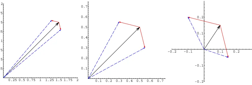
4.1. The effects of two different noise vectors with the same amplitude but different

phase on various inputs. .. .. .. .. .. .. .. .. .. .. .. .. .. .. .. .. 15

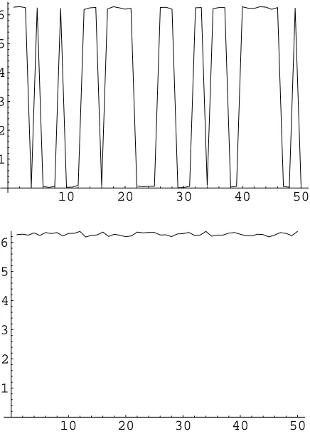
4.2. Variance in measured phase is greatly reduced by calculating over a 5 GP window

rather than a 2 GP window. .. .. .. .. .. .. .. .. .. .. .. .. .. .. .. 16

4.3. Examples of the filters discussed in section 4.2. .. .. .. .. .. .. .. .. .. 17

4.4. Phase variance and delta-phase variance vs harmonic number. .. .. .. .. .. 19

5.1. The Mean Probability Signature closely approximates a histogram of the number

of values in the average delta-phase variances which are below a threshold. .. .. 21

5.2. Mean Probability Signatures from three different sounds. .. .. .. .. .. .. 21

6.1. The Mean amplitude for an utterance of /m/ (left) and /n/ (right) with a clear

difference around the seventh harmonic. .. .. .. .. .. .. .. .. .. .. .. 23

6.2. The Mean amplitude for an utterance of /m/ (left) and /n/ (right) lacking clear

(9)

6.3. The mean time delays for an utterance of /m/ (left) and /n/ (right). (x-axis is

harmonic number) .. .. .. .. .. .. .. .. .. .. .. .. .. .. .. .. .. 24

6.4. The filtered time delays vs GP number for an utterance of /m/ (left) and /n/

(right). .. .. .. .. .. .. .. .. .. .. .. .. .. .. .. .. .. .. .. .. 25

6.5. The result of deciding that each GP is either /m/ (1) or /n/ (-1) and then performing a

moving-average 5 filter, in effect “voting” among each group of 5 consecutive GPs

for an utterance of /m/ (left) and /n/ (right). .. .. .. .. .. .. .. .. .. .. 25

6.6. The average phase variance vs GP number for an utterance of /m/ (left) and

/n/ (right). .. .. .. .. .. .. .. .. .. .. .. .. .. .. .. .. .. .. .. 26

6.7. The target probability signature for an utterance of /m/ (left) and /n/ (right). (x-axis

is frequency) .. .. .. .. .. .. .. .. .. .. .. .. .. .. .. .. .. .. .. 27

6.8. Comparison to target probability signatures for an utterance of /m/ (left) and

/n/ (right). .. .. .. .. .. .. .. .. .. .. .. .. .. .. .. .. .. .. .. 27

6.9. The difference of the /m/ and /n/ target probability signature comparisons vs GP

(10)

List of Tables

7.1. The results from phase 1. The comparisons are presented in graphical (rather than

tabular) form for better visual recognition. .. .. .. .. .. .. .. .. .. .. .. 31

7.2. The results from phase 2 of the experiment. .. .. .. .. .. .. .. .. .. .. 32

7.3. The p-values for concluding classification accuracy is better than simply guessing

(11)

Chapter 1. Introduction

1.1. Introduction to Speech Processing

One division of speech sounds is the distinction between voiced and unvoiced (or

voiceless). Voiced sounds are made by vibrating the vocal chords, whereas unvoiced sounds are

made without vibrating the vocal chords. The vibration of the vocal chords produces glottal

pulses, where one glottal pulse (GP) is the sound produced by a single vibration of the vocal

chords. The spectrum of voiced speech is the product of the glottal pulse (the driving signal) and

the mouth shape (the filter). To prevent aliasing in any processing of the spectrum of a voiced

speech sample, the processing must be done over the period of only one glottal pulse at a time.

To divide the sample into glottal pulses, the glottal pulse periods (GPPs) are computed by the

algorithm described in [5].

1.2. Introduction to Lip Synchronization

In linguistics, a single unit of sound is called a phoneme. The corresponding concept

in lip synchronization, the position of the tongue, mouth, and jaw, is called a viseme (visual

phoneme). Several phonemes may map to the same viseme. For example, /p/, /b/, and /m/

form a single viseme. Lip synchronization is the process of deriving visemes from sounds

in a voice data stream, whereas speech recognition must produce phonemes from the data

stream. Lip synchronization is different from speech recognition because multiple acoustically

similar phonemes may share a single viseme and not require differentiation, and each produces

different output.

Lip synchronization can be either text-based, where the text of the speech is

(12)

synchronization is more closely related to text-to-speech technologies than to voice recognition

technologies. Text-independent lip synchronization is much more difficult than text-based lip

synchronization. This paper was motivated by work with a text-independent lip synchronization

system.

The lip synchronization system, as described in [1, 2, 3, 4], has shown that moments of the

spectrum of a voice sample can be used to derive its associated viseme. After dividing the voice

sample into glottal pulses, the moments are computed for the spectrum of the sample during

each glottal pulse period. The first moment, m1, is the mean of the spectrum. The second

principal moment about the mean, m2, is the variance. The spectrum of each glottal pulse period

is distilled into a single point in m1-m2 space. The points for a voice sample can be interpolated

to produce a track in m1-m2 space.

The track in m1-m2 space may be mapped onto a continuous predictor surface for each of

three mouth shape parameters: jaw position, horizontal lip opening, and vertical lip opening.

(There are actually two parameters for horizontal mouth opening, but only one of them is

currently being treated as an independent variable.) There may be several different predictor

surfaces for the different types of speech, e.g. vowels, fricatives, and nasals. Problems may

arise, however, when multiple visemes share the same region in m1-m2 space. This is the case

with the nasals, /m/ and /n/. This problem has motivated this research into the use of the phase

characteristics of the spectrum in order to distinguish /m/ and /n/.

1.3. Introduction to Phase

Voiced speech is the result of applying a filter (supplied by the mouth and nasal cavities)

to the driving signal produced by the vocal chords (glottal pulses). The filter is important in

determining mouth shape parameters. The discrete Fourier transform is used to extract the

filter parameters from input speech. When a discrete Fourier transform is applied to a segment

of speech input of length n, the result is a list ofn_⁄2complex numbers that define the amplitude and phase ofn_⁄2harmonics. If the complex number x +yi is treated as a vector in the complex

plane, the amplitude is the magnitude of the vector,

√

x2 +y . The phase angle of the vector is2

measured in radians as arctan(y⁄x). While the measurement of phase from the discrete Fourier

(13)

restricted in range, it may exhibit2πjumps. The phase of the actual filter usually does not have

any discontinuities.

Both the amplitude and phase from the discrete Fourier transform are necessary to

reconstruct the filter. Two different sounds can be produced by two filters with similar amplitude

characteristics but different phase characteristics. This is likely the case with /m/ and /n/.1_Since

/m/ and /n/ are produced by air flowing through multiple paths in the mouth and nasal cavities,

the filter is a non-minimum phase filter.2_{This makes it much easier for the two different filters}

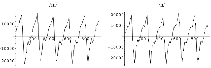
to have similar amplitude characteristics, but different phase characteristics. Figure 1.1 shows

the similarity in the /m/ and /n/ waveforms.

Most previous work has used the amplitude characteristics for speech analysis. Prevailing

wisdom among linguists and speech processing experts is that the phase component of speech

does not carry useful information. Previous experiments in which the phase of speech signals

was intentionally altered have showen that human listeners do not rely on phase information

to determine the content of speech. From this work, one can conclude that human speech

perception is dominated by the amplitude portion of the input. This does not imply useful

information is not carried by the phase component. This work uses the phase characteristics

of speech in a different way. The phase of the filter provided by the mouth and nasal cavities

is computed, minimizing the contribution of the vocal chords. Phase may not be perceptible by

1_{Previous work [1, 2, 3, 4] has demonstrated that the moments of the amplutude spectrum of /m/ and /n/ are, in fact,}

not distinguishable.

2_{See Appendix A, page 38 for an explaination of minimum phase filters}

/m/

200 400 600 800

-20000 -10000 10000

/n/

200 400 600 800

-20000 -10000 10000 20000

(14)

the human ear, but it is an important part of the filter characteristics. For example, the /m/ and

/n/ sounds have almost identical amplitude spectra, so the phase contribution to the filter may

be significant.

1.4. Experiment Overview

In order to attempt to distinguish /m/ and /n/, an experiment was designed wherein various

measures were obtained from speech samples from several utterances of several speakers.

These measures were then compared with the measures obtained from other speech samples and

used to classify the new samples as /m/ or /n/.

The speech samples were processed by first segmenting them into individual glottal

pulses. The phase spectrum was then computed for each glottal pulse over several harmonic

frequencies. These phases were then corrected for various measurement artifacts and low signal

artifacts, as described in Chapters 3 and 4. Measurements derived from phase were averaged

together for each speaker in order to produce comparison functions for /m/ and /n/. Additional

samples were then processed to obtain phase, and compared with the comparison functions.

The techniques used in the experiment correctly identified the speech samples

(15)

Chapter 2. Background

2.1. Previous work on Lip Synchronization

Lip Synchronization Research has taken several directions, including both text-based and

text-free methods.

Several systems couple text-to-speech sound generation and lip synchronization [17, 18].

Since the text-to-speech engine must already compute phonemes, the only remaining problem

is to map the phonemes to visemes and then synchronize the audio and video streams.

[9] presents a text-free solution in which the speech is divided into frames such that each

frame of rendered video corresponds to one audio frame. The audio frames are represented as

12-dimensional cepstrum vectors and input into a time-delay neural network which uses hidden

Markov models. The system was trained using only one speaker and [9] does not present any

results of trying to use the system with a different speaker.

2.2. Previous work using moment space

McAllister, et al. [1, 2, 3], present a text-free lip synchronization system which uses spectral

moments of the speech to estimate visemes. Interpolating the first and second moments (m1,

m2) calculated for the spectrum of each glottal pulse period yields a track in m1-m2 space. For

any given type of sound (e.g. vowels, nasals) the m1-m2 space maps onto a smooth predictor

surface for the mouth shape parameters. Different types of sound may map the same region

in m1-m2 space to different visemes, so the input speech must be separated and tagged by type

before generating a mouth shape predictor surface. Tracks for different speakers uttering the

same sound are similar in overall shape and position, but are significantly different in terms of

(16)

[16] explores a method of providing speaker independence in McAllister’s text-free

automated lip synchronization system. Speaker independence is achieved by creating a

mapping of the spectral moments of the speaker’s voice onto those of an ideal “standard”

speaker.

The advantage of using spectral moments is that every step of the process in finding

the moments is an integration over the signal. This means that the result is less susceptible to

signal noise than other techniques. Using spectral moments also carries some disadvantages.

As mentioned earlier, the spectral moments for the same sound are different between different

speakers. Also, the moments of different sounds belonging to different types of sound (vowels,

fricatives, etc.) may be similar. The speech must be separated by sound type before any

meaningful comparison can be made between spectral moments of different sounds and the

corresponding visemes [6].

The regions in m1-m2 space for /m/ and /n/ coincide, thus a different approach must be

taken to distinguish /m/ and /n/.

2.3. Previous work on phase

Several authors have concluded that phase information in speech is not necessary to

maintain intelligibility, while others have indicated that it does contain significant information.

In the late 1800’s, Helmholtz observed that human hearing is insensitive to phase in speech, at

least for “the ’musical’ portion of the sound” (i.e. for vowels) [19, p.419]. Additional studies

have generally supported this observation [19]. This is not to say that the phase component of

speech contains no useful information. On the contrary, synthesized speech which contains

phase information most like human speech is more intelligible and natural sounding than

synthesized speech which does not [7, 10]. Furthermore, speech synthesized by taking only

the phase component of natural speech, while sounding strange, retains a high degree of

intelligibility [14].

Relatively few attempts have been made to extract useful information from the phase

component of speech. In [12], Murthy uses group delay, the negative derivative of phase, to

(17)

is itself derived from the magnitude spectrum of the Fourier transform of the speech signal. In

[13], the phase of the speech signal itself is used. Murthy discovered that “the rapid fluctuations

in the log magnitude spectrum and the group delay function are caused by the zeroes of the

z-transform of the excitation components of the speech signal. Zeroes close to the unit circle

in the z-plane produce large amplitude spikes in the group delay function and mask the group

delay information corresponding to the vocal tract system.” Since, in sample data, nasals have

zeros in the transform, Murthy did not extract useful group delay information for them.1

In a later paper [11], Murthy creates a modified group delay function to suppress these

zeros. His reasoning is that “they are not of much interest in speech analysis, since in speech,

zeroes occur only in the production of nasals”. However, these zeros may therefore be of great

interest when attempting to distinguish /m/ and /n/. Murthy uses the modified group delay

function in a phoneme recognition system.

Some groups have used phase which was not gleaned from Fourier transform phase, but

rather from time delay on the speech signal itself [8, 20, 21, 22]. These groups compare the

speech signal with offsets of itself to create vectors in a multi-dimensional “Reconstructed

Phase Space” representation of the speech. They then take various measures of the tracks in

RPS and use these to attempt to distinguish phonemes, with varying degress of success.

(18)

Chapter 3. Extracting Phase

Extracting a useful phase signal from speech input is a non-trivial problem. Unlike

amplitude, phase is extremely time-sensitive. That is, phase changes linearly with delay and

proportionally with harmonic frequency. While amplitude has a range of0..

∞

, measured phase has a range of−π..π. Furthermore, since measured phase has a constrained range but the actual phase of the filter does not, the measured phase can exhibit2π jumps even though the actual

phase is continuous. Finally, phase is unreliable at low amplitudes because a small change in

position in the complex plane can correspond to a large change in phase angle when amplitude

is small. Each of these issues will be detailed, and solutions presented.

3.1. Subtracting phase changes caused by phase delay

Voiced speech is the result of applying a filter (supplied by the mouth and nasal cavities)

to the driving signal produced by the vocal chords (glottal pulses). The filter is important in

determining mouth shape parameters. Therefore, in order to eliminate the effect of the driving

signal from the calculations, the speech signal is processed over a single glottal pulse period

each time.1

In order to reduce the impact of noise in the calculations, an average value is computed

across the glottal pulse. For a glottal pulse of length x samples starting at time t, amplitude and

phase are computed over x different signal windows. Each window is of length x, but starts at

time t+i where i is between0and x− 1. Amplitude and phase are then averaged over the glottal pulse period. This does not present any problems for amplitude because it typically does not

vary significantly across the glottal pulse. Phase, however, does vary across the glottal pulse, as

shown in figure 3.1. To obtain meaningful information from the averaging process, the part of

the phase variation caused by moving the window (that is, phase delay) must be determined and

1_{Actually, two contiguous glottal pulses are used so that an average value for the glottal pulse can be obtained by sliding}

(19)

removed.

The phase delay function may be derived by beginning with time delay, a measure of

the difference in starting time between two different signal windows. Time delay is related

to phase by the equation D(ω) = − ∂Φ

∂ω , in whichω is equivalent to harmonic number when time is expressed in terms of the glottal pulse period (i.e. the window size in samples). From

this equation it can be derived that Φ(ω) = −

∫

D(ω)∂ω . The expected phase function can be computed, examining what happens to phase when time delay increases as the window

advances. D_i₊₁(ω) = D_i(ω) + ∆t ⇒ Φ_i₊₁(ω) = −

∫

D_i(ω)∂ω −

∫

∆t∂ω = Φ_i(ω) − ∆tω The effects of the moving window are removed by subtracting the∆tωterm, remembering that ∆

t must be expressed in terms of the window size as − 2πδ

windowsize+ 1whereδis the number of

samples the window has moved. The∆t term is negative because it represents advancing the

signal, rather than delaying it, thus, it is a negative time delay. The phase at the first harmonic

completes its revolution through an entire 2 π in windowsize increments. This requires

windowsize+ 1samples, thus accounting for the 2π

windowsize+ 1contribution to∆t.

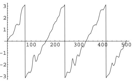
After removing the effect of the sliding window from the measured phase, the range

of the result must be re-constrained. The measured phase has constrained range and

experiences 2 π jumps, but the “delay corrected” phase calculation does not. The resulting

phase, therefore, will have a2πjump every place the measured phase does, as shown in figure

3.2. Since there is no particular advantage to using a range of −π.. πrather than0.. 2π, the later is used because it is more efficient to compute. Both ranges will exhibit some problems

100 200 300 400 500

-3 -2 -1 1 2 3

(20)

discussed in a later section. This gives the final formula for computing the corrected phase:

mod(measuredPhase− 2πδω

windowsize+ 1, 2π). A more rigorous derivation is given in appendix

B on page 39.

The formula for delay corrected phase can be verified by constructing an input signal using

a known driving signal and filter, such as in figure 3.3. The phases for several harmonics for one

pulse period of this function are shown in figure 3.4, along with the corresponding expected

phases. The corrected phases corresponding to figure 3.4 are shown in figure 3.5.

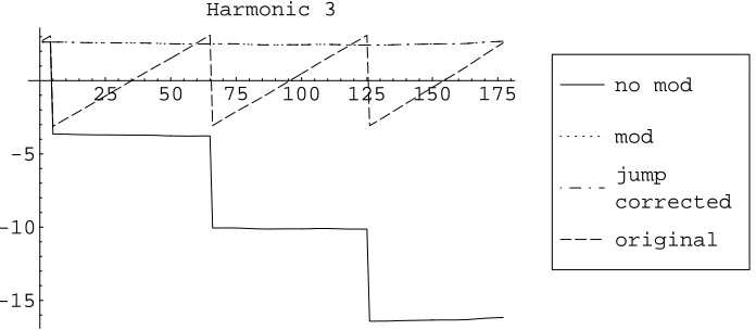
25 50 75 100 125 150 175

-15 -10 -5

Harmonic 3

original jump corrected mod

no mod

Figure 3.2. A comparison of the corrected phase vs input window start sample with and without correction for phase delay (as described in section 3.1). The figure shows uncorrected phase (“original”), phase corrected for phase delay without correcting for2πjumps, both before and after having the range restricted to0..2π(“no mod” and “mod”, respectively), and phase corrected for phase delay and corrected for2πjumps (“jump corrected”). In this example, the “mod” and “jump corrected” lines coincide because the “mod” line is not near a2πboundary (and thus does not exhibit any jumps).

100 200 300 400 500 0.02

0.04 0.06 0.08 0.1 0.12 0.14

(21)

Harmonic 1:

20 40 60 80 100 120

-3 -2 -1 1 2 3

20 40 60 80 100 120

-3 -2 -1 1 2 3 Harmonic 2:

20 40 60 80 100 120

-3 -2 -1 1 2 3

20 40 60 80 100 120

-3 -2 -1 1 2 3 Harmonic 3:

20 40 60 80 100 120

-3 -2 -1 1 2 3

20 40 60 80 100 120

-3 -2 -1 1 2 3

Figure 3.4. Some of the (uncorrected) phases of the first pulse period of the signal shown in figure 3.3 appear on the left. The corresponding phases expected due to phase delay are shown on the right. (Shown as phase vs sample number)

3.2. Correcting for Jumps

One of the first steps in the processing of phases, as in the processing of amplitudes, is to

average the phases to obtain a single phase per harmonic per glottal pulse. Before this can be

(22)

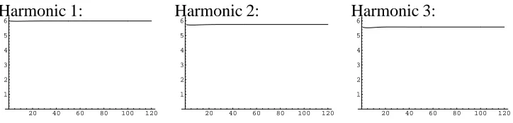
Harmonic 1:

20 40 60 80 100 120 1

2 3 4 5

6 Harmonic 2:

20 40 60 80 100 120 1

2 3 4 5

6 Harmonic 3:

20 40 60 80 100 120 1

2 3 4 5 6

Figure 3.5. The corrected phases corresponding to the phases in figure 3.4. The results agree with the phases calculated for the constructed input signal. (Shown as phase vs sample number)

Since the phase represents an angle in polar coordinates, a change of ±2πin phase is not

really a change. Values which are overπapart are more likely to have crossed a2πboundary

and should be less thanπapart. For example, consecutive values of (2π − 0.1)and0.1will be calculated as a change of(0.2 − 2π), when the actual change in phase is more likely to have been

+ 0.2.

To eliminate the2πjumps, the phase signal is modified so that no sample is further thanπ

away from the previous sample. This restriction means that the phase shift between to samples

at the highest harmonic frequency considered is assumed to have magnitude less than π. The

results are shown in figure 3.6.

The correction for2πjumps must be performed any time two angles are compared. The

next step in the processing of phases is to compute time delay, the difference in phase between

successive harmonics. Since the difference in phase is a difference between two angles, the

result must be corrected for2πjumps.

3.3. Starting the glottal pulse at minimum phase

As mentioned previously, speech input is separated into glottal pulses, and the phase

calculations are done over one glottal pulse at a time. The glottal pulse tracker used to identify

glottal pulse boundaries is accurate to within a few samples. However, the tracker only identifies

the length of the glottal pulses. It would be ideal to also identify the start of the glottal pulse,

defined as the window where the phase calculation yields minimal time delay, i.e. the slope of

(23)

10 20 30 40 50 1

2 3 4 5 6

10 20 30 40 50

1 2 3 4 5 6

Figure 3.6. A signal with range 2 π ±.0 1before and after correcting for2 πjumps. The x axis is in the time domain.

averaging of the derived phase characteristics.

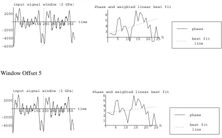
Figure 3.7 shows the results of moving the input signal window by a few samples before

computing phase. A line is fit through the phases using the amplitudes as weights. The line

is weighted because phase is more likely to be correct when the amplitude is high. This is

discussed in further detail in a later section. Figure 3.7 also shows the slope of this line in

relation to the amount the input signal window is offset. The window is closest to the actual start

of the glottal pulse when the slope of the line is closest to 0.

Finding the exact beginning of the glottal pulse is computationally intensive. It is not clear

that it is necessary to be so precise. Adequate results have been obtained by using a combination

of finding an approximation for the beginning of the glottal pulse and simply subtracting the

(24)

Window Offset 3

50 100 150 200 250 300 350 time

-6000 -4000 -2000 2000

input signal window H2 GPsL

5 10 15 20 25h 3

4 5 6

Phase and weighted linear best fit

best fit line phase

Window Offset 5

50 100 150 200 250 300 350 time

-4000 -2000 2000

input signal window H2 GPsL

5 10 15 20 25h 1

2 3 4 5 6

Phase and weighted linear best fit

best fit line phase

(25)

Chapter 4. Enhancing the Phase Signal

By far, the most difficult part of extracting useful information from phase is dealing with

areas of the input signal which have a low signal to noise ratio. The amplitude component of

speech does not present much of a problem in this area, since the amplitude is miniscule in areas

of low or no signal. Phase, however, is essentially random in these areas. More accurately, any

phase information from a weak signal is easily overwhelmed by noise and thus appears to be

random. Figure 4.1 shows why this is so.

Several techniques are presented which attempt to reduce the amount of error in the

extracted phase signal.

4.1. Strengthening the signal

One way of increasing the signal strength is to combine information from multiple glottal

pulses. In order to do this, one may exploit a property of the Fourier transform when applied

to periodic signals. For a signal consisting of a periodic function f with period p, the sums of

0.25 0.5 0.75 1 1.25 1.5 1.75 2 0.25

0.5 0.75 1 1.25 1.5 1.75 2

0.1 0.2 0.3 0.4 0.5 0.6 0.7 0.1

0.2 0.3 0.4 0.5 0.6 0.7

-0.2 -0.1 0.1 0.2

(26)

certain harmonics of the Fourier transform with window size n ∗ p display certain properties.

The value for harmonic h∗n (“non-cancelling harmonics”) is n times the value for harmonic h

of the Fourier transform of a single cycle of f using window size p. It is also true that the other

harmonics (“cancelling harmonics,” i.e., ones which are not an integer multiple of n) are zero.1

This property has already been used for n = 2to find the glottal pulse lengths. Similarly, the

glottal pulse length may be recomputed over a window of 5 GPs. In practice, this value never

deviates from the original GP length estimate by more than 1, thus indicating the high quality

of the glottal pulse tracker. One also can calculate phase information using a 5 GP window,

processing the results as described in previous sections. This reduces variance in the phase and

increases signal strength as illustrated in figure 4.2

4.2. Filtering weak signals

In some cases, the signal remains weak even after computing over 5 glottal pulses. In these

cases it is necessary to filter unusable portions of the phase signal. Several filtering methods are

presented below. The results of these methods are compared in figure 4.3.

1_{See Appendix C (page 41) for further details.}

20 40 60 80 100 120 0.25

0.5 0.75 1 1.25 1.5 1.75

2 phase variance, n = 5

20 40 60 80 100 120 0.25

0.5 0.75 1 1.25 1.5 1.75

2 phase variance5, n = 5

(27)

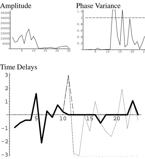
Amplitude

5 10 15 20 25 5000

10000 15000 20000 25000 30000 35000

Phase Variance

5 10 15 20 25 0.2

0.4 0.6 0.8 1 1.2

Time Delays

5 10 15 20

-3 -2 -1 1 2 3

Figure 4.3. Examples of the filters discussed in section 4.2. The amplitude and phase variances are provided for reference. The results of applying the filters to time delays are overlayed in the chart. The original time delays are in gray. The amplitude filtered time delays are the dotted line. The phase variance filtered time delays are the heavy black line. The x-axis on all of the charts is harmonic number.

4.2.1. Filter by amplitude

Since the signal can be assumed to be good when the amplitude is high, the phase signal

is filtered based on a simple amplitude threshold. Selecting a single threshold for all inputs is

problematic, as samples can vary widely in input speech volume. This problem can be reduced

by selecting the threshold as a percentage of the maximum amplitude of the input sample, but

this requires a priori knowledge of the entire sample, and issues could remain if the amplitude

varies widely within the sample.

This method has the advantage of being simple and fast. However, it makes the

contribution of the amplitude to the resulting signal very large. The techniques used to extract

shape parameters from the signal may pick out the shape of the filter over the shape of the phase

information. In particular, the interesting region in the frequency spectrum for distinguishing

/m/ and /n/ may have low amplitude. It is desirable to find a way to filter the signal which

(28)

4.2.2. Filter by phase variance

This method removes the reliance on amplitude information completely. One of the first

steps in the processing is to average the phases within each glottal pulse to produce a single

number per harmonic per glottal pulse. In addition to the mean, the variance, which will

be referred to as the phase variance, may also be computed. The phase variance is inversely

correlated with amplitude in speech input. The phase signal (after averaging) can then be

subjected to a filter based on a threshold of phase variance. Phase variance and the filtered phase

signal are actually computed separately, with separate thresholds, for the phases computed using

the normal 2 GP window and the extended 5 GP window.

Variance in the phase for a harmonic can come from two sources: noise or change in

phase across the glottal pulse. A change in phase across the glottal pulse should result in a

constant slope on the corrected phase. Noise is assumed to produce a more random phase signal,

with a high variance. (These generalizations have held true in all of the author’s experimental

observations.) Since the phase variance is to be used as a measure of signal strength, any

contribution from the change in phase across the glottal pulse should be minimized or removed,

since such a change is a legitimate signal. This can be done by fitting a line to the phase and

subtracting it before computing the variance, thus removing any slope from the phase.

The phase variance is easy to compute, and removes the reliance on amplitude information.

Choosing the appropriate phase variance threshold appears to be relatively straightforward,

and has yielded reasonable results on the input samples that have been considered thus far.

Computing the variance of the sine and cosine components separately may yield a more precise

descriminator, but it is not clear that this is necessary. Future work on this filter may include

applying a moving average filter to the phase variances before applying the threshold.

A variation on the phase variance filtering method is to filter by variance in the change in

phase between harmonics (“delta-phase”). If the features to be extracted from the phase signal

are to be computed based on delta-phase (because, for example, the shape of the curve is deemed

more interesting that the actual values), then it makes sense to filter on delta-phase. There are

differences when filtering by phase vs. delta-phase, but they do not appear to be significant. As

shown in figure 4.4, they appear highly correlated. Also, figure 6.3 shows the results of filtering

(29)

5 10 15 20 25 30 35 0.2

0.4 0.6 0.8 1 1.2

Phase Variance

5 10 15 20 25 30 0.2

0.4 0.6 0.8 1 1.2

Delta-phase Variance

(30)

Chapter 5. Other Metrics from Phase

Rather than trying to eliminate areas of low signal, as in section 4.2, the author instead

hypothesizes that the weak signal appears at the most inopportune frequency because it is

caused by the presence of an anti-formant in the voice filter. The phase variance (or delta-phase

variance) may be used as an indirect indication of the presence of an anti-format in the

voice filter.

Thus, when filtering by phase variance (as described in section 4.2.2), it is just as interesting

to consider the number of points which are filtered as it is to consider the resulting filtered time

delays. To compute this value, however, it is necessary to have completed processing of an entire

utterance in order to count the number of filtered points. The probablity signature, as described

below, is an attempt to produce a function which approximates the same shape as the histogram

of the number of filtered-in points vs harmonic.

5.1. Computing the Mean Probability Signature

The probability signature is computed over a single glottal pulse as a function of the

probablity that at harmonic n, the variance v_n is below a threshold. Specifically this value is

PS(n) = 2(1 − CDF(

√

v_n)), where CDF is the cumulative distribution function on a normal distribution centered about the origin with standard deviation 0.8. A cumulative distribution

function is the integral of the probability distribution function to the left of the given value. Note

that the probability signature is not actually a measurement of probability, although it does have

a0..1range and is positively correlated with probability.

The Mean Probablity Signature is the average value of the probability signatures of the

average delta-phase variances for each glottal pulse, mapped to the frequency domain (from the

harmonic domain) using the average glottal pulse length. The shape of the Mean Probability

(31)

variances which are below a threshold, as shown in figure 5.1 (which are still expressed in terms

of harmonic number rather than frequency).

5.2. Target Probability signatures

Using the Mean Probability Signatures from several utterances of a sound, one can

compute a signature which we expect the variance vs. frequency plot of any given GP of that

sound to match, the Target Probability Signature. This allows one to compare phase variance as

another tool to attempt to distinguish different sounds.

To compute Target Probability Signatures, collect the Mean Probability Signatures from

three utterances of each sound and average them to obtain one signature for each sound. Figure

5.2 illustrates three different sounds. Then create an interpolated function for each sound, since

the function is in the frequency domain, which is (for all practical purposes) continuous, rather

than in the harmonic domain, which is discrete. These are the Target Probability Signatures.

5 10 15 20 25 30 20 40 60 80 100 120

delta-phase variances below threshold

5 10 15 20 25 30 0.2

0.4 0.6 0.8

1 Mean Probability Signature

Figure 5.1. The Mean Probability Signature closely approximates a histogram of the number of values in the average delta-phase variances which are below a threshold. (x-axis is harmonic number)

1000 2000 3000 4000 0.2

0.4 0.6 0.8 1

ee

1000 2000 3000 4000 0.2

0.4 0.6 0.8 1

m

1000 2000 3000 4000 0.2

0.4 0.6 0.8 1

n

(32)

Now define a comparison function which is a RMS error measurement between the input

probability signature and one of the Target Probability Signatures. Any probability signature,

whether from a single glottal pulse or an average across all glottal pulses, may be compared

using the comparison function. The Target Probability Signature which results in the lowest

value returned from the comparison function belongs to the sound which most closely matches

the input sound.

5.3. Time delay signatures

Time delay signatures may be computed in the same manner as the probability signatures

described above, except using the variance of time delay rather than the phase variance, to give

yet another tool for comparison. In preliminary investigation, time delay signatures appeared

to have an ability roughly comparable to that of probability signatures to distinguish different

phonemes. Since this ability was not obviously better, no additional work was done with time

delay signatures. Additional experimentation is required to fully explore the uses of time

(33)

Chapter 6. Attempting to Distinguish /m/

and /n/

Several methods for distinguishing /m/ and /n/ were attempted using voice samples from

a single speaker, with varying degrees of success. All of them involve examining the region

around 600Hz, though some may do this as part of a larger overall comparison. The results in

this chapter are based upon a very small collection of input samples, and are primarily intended

to identify a classification method to be tested with more samples from multiple speakers in

Chapter 7. Unless otherwise noted, the figures in this chapter are representative examples of

trends which were observed to hold true over at least three samples.

6.1. Compare amplitude

In some samples, the amplitude around 600 Hz is markedly different, as shown in figure

6.1. Note the high secondary peak present around the 7th harmonic in /m/ which is not present

in /n/. However, in other samples, such as those in figure 6.2, this behavior not as clear. The

unreliability of this method of distinguishing /m/ and /n/ makes it unsuitable as a primary

classification mechanism.

5 10 15 20 25 30 35harmonic 20000

40000 60000 80000 100000

Mean amplitude

5 10 15 20 25 30 35harmonic 20000

40000 60000 80000 100000

Mean amplitude

(34)

5 10 15 20 25 30 35harmonic 20000

40000 60000 80000 100000 120000

Mean amplitude

5 10 15 20 25 30 35harmonic 10000

20000 30000 40000 50000 60000

Mean amplitude

Figure 6.2. The Mean amplitude for an utterance of /m/ (left) and /n/ (right) lacking clear difference around the seventh harmonic.

6.2. Compare peak in time delay

The peak in time delay for /m/ is generally higher than the corresponding peak for /n/, as

shown in figure 6.3. The peak in figure 6.3 is on the 5th harmonic (actually the difference in the

5th and 6th harmonics). To ensure that this peak is a distinguishing characteristic between /m/

and /n/ throughout the entire input sound and not an artifact which can only be reproduced by

averaging over the entire sound, two things must be examined. First, the time delay vs. glottal

pulse should show little variation across the input sound at the 5th harmonic. Second, there

should be enough values for time delay after the filtering has occurred so that any sub-segment

of the input sound of sufficent length has at least one filtered-in value. These properties are

illustrated in figure 6.4.

5 10 15 20 25 30

-3 -2 -1 1

average of filtered time delays

5 10 15 20 25 30

-2 -1 1 2 3

average of filtered time delays

(35)

20 40 60 80 100 120 -3 -2 -1 1 2 3

filtered time delays, n = 5

20 40 60 80 100 120

-3 -2 -1 1 2 3

filtered time delays, n = 5

Figure 6.4. The filtered time delays vs GP number for an utterance of /m/ (left) and /n/ (right).

This difference in peak values is considerably less clear when using time delay calculated

using a 5 GP window; however, for the nasal sound in isolation, it appears that applying a

threshold will suffice. Figure 6.5 shows the result of deciding that a GP is either /m/ (1) or /n/

(-1) and then performing a moving-average 5 filter, in effect “voting” among each group of 5

consecutive GPs.

When examining sounds containing transitions from a vowel, however, it is clear that

knowledge of the leading vowel is required, as the value of the time delay peak is different

depending on the leading vowel. The change in time delay from the vowel appears to be greater

for /m/, but this requires a larger sample size to say with any certainty. There are several things

about this method which make it undesirable as a primary classification mechanism. It employs

thresholds, which are notoriously difficult to optimize, and may vary by speaker. The differing

peak values for vowel-nasal samples appear to vary based on leading vowel, but the direction

and extent of the variance may also be speaker dependent. Training a classification system

20 40 60 80 100

-1 -0.75 -0.5 -0.25 0.25 0.5 0.75 1

20 40 60 80 100

-1 -0.75 -0.5 -0.25 0.25 0.5 0.75 1

(36)

based on this method could require training on each leading vowel separately. Additionally,

it means the nasal classification system is predicated on having a working vowel classification

system. It is desirable to find a classification method which requires less per-speaker training,

which in turn means a smaller sample population required for statistical relevance.

6.3. Compare phase variance

As shown in figure 6.6, the average phase variance for /m/ and /n/ is markedly different

in the 600 Hz range. As in the case of time delay, it appears that a threshold will suffice. This

method greatly reduces the amount of per-speaker training which may be required, however,

as noted previously, thesholds are notoriously difficult to optimize and may still require

per-speaker training. In this case, the threshold is difficult to optimize because the optimization

problem is in two dimensions: First, the frequency region of interest may vary by speaker due

to physical differences in the mouth and nasal cavities. Second, the phase variance may be

increased for all harmonics by the addition of background white noise. These problems may be

overcome by comparing probability signatures (which are based on phase variance) instead.

6.4. Probability signature comparisons

Using a the target probability signatures (shown in figure 6.7) and a comparison function,

the probability signature for any particular GP can be compared against both the /m/ and /n/

target probability signatures.

20 40 60 80 100 0.25

0.5 0.75 1 1.25 1.5 1.75 2

20 40 60 80 100 0.25

0.5 0.75 1 1.25 1.5 1.75 2

(37)

1000 2000 3000 4000 0.2

0.4 0.6 0.8 1

m

1000 2000 3000 4000 0.2

0.4 0.6 0.8 1

n

Figure 6.7. The target probability signature for an utterance of /m/ (left) and /n/ (right). (x-axis is frequency)

The comparison function takes two probability signatures as arguments (the known target

probability signature and the probability signature of the unknown input sample) and yields a

scalar, the RMS error of comparing its two arguments. Thus, lower values represent a closer

fit. Figure 6.8 illustrates the result of performing these comparisons for each GP in the input

sample.

This comparison becomes clearer if one instead considers the value of the /m/ comparison

minus the /n/ comparison. Figure 6.9 shows for each GP the value obtained by computing the

/m/ comparison then subtracting the value computed for the /n/ comparison. Subtracting the

values of the /n/ comparison from the /m/ comparison yields a simple way to classify the input

speech as /m/ or /n/ when the value is below or above zero, respectively. The relative simplicity

of this method makes it ideal for further exploration in Chapter 7.

20 40 60 80 100 120 GP 0.25

0.3 0.35 0.4 0.45 0.5

/m/ and /n/ comparisons vs GPHmoving avg-3L

20 40 60 80 100 120 GP 0.25

0.3 0.35 0.4 0.45

/m/ and /n/ comparisons vs GPHmoving avg-3L

(38)

20 40 60 80 100 120

-0.08 -0.06 -0.04 -0.02 0.02 0.04

/m/ minus /n/

20 40 60 80 100 120

-0.04 -0.02 0.02 0.04 0.06 0.08 0.1

/m/ minus /n/

(39)

Chapter 7. Applying the Technique to

Real-World Samples

The methods previously described in chapter 6 were tested using a single speaker (the

author). In order to determine if the results obtained are truly useful, additional speakers must

be considered. An experiment which uses the target probability signatures to distinguish /m/

and /n/ is described in this chapter.

7.1. Experiment Design

Voice samples were recorded in a low-noise environment (a sound booth) from four male

and four female speakers.1_{The speakers were instructed to read a series of statements in a}

natural voice, as well as to recount a children’s fairy tale (without script).2_{The voice samples}

were recorded as.wavfiles at a sampling rate of 20000 Hz using 16 bits per sample. Waveform

editing (i.e. isolating speech segments) was done using Audacity, an open-source audio editor.

In the first phase of the experiment, segments of the pure /m/ and /n/ nasal sounds were

isolated for each speaker. Between three and six samples of each sound were found, and used

to create a mean probability signature. Target probability signatures where then computed, as

described in section 5.2, for /m/ and /n/ for each speaker. For each speaker, the mean probability

signatures of the samples where then classified using the target probability signatures which

were just computed for that speaker. A high classification accuracy is expected, since the mean

probability signatures were used to create the target probability signatures. This serves as a

sanity check, to ensure that the techniques which worked for a single speaker can be generalized

to multiple speakers (although in a speaker-dependent way).

1_{Recordings were funded by NSF grant BCS-0213941.}

(40)

In the second phase of the experiment, additional samples were isolated from each speaker.

Between 20 and 50 samples of vowel to nasal transitions were isolated for each speaker, using

a mix of initial vowels. These new samples were then compared to the target probability

signatures generated in phase 1. The resulting tracks of the comparison were then examined by

hand to determine if each classified the sample as /m/ or /n/ correctly.

7.2. Results

7.2.1. Phase 1

Isolating pure nasal sounds 200ms long proved difficult. Nasals are not frequently

sustained for such a duration in natural speech, except as filler (e.g. “um”, “and”). Once the

samples were isolated, however, the target probability signatures were able to identify /m/ vs.

/n/ with approximately 91% accuracy. These results are presented graphically in table 7.1. In

the table, each row shows results for a different speaker. The first and second columns show the

target probability signatures for /m/ and /n/ samples, along with the mean probability signatures

used to compute them. The third and fourth columns show the results of comparing the /m/

and /n/ input samples, respectively, to both the /m/ and /n/ target probability signatures. The

datapoints in the right hand columns are connected by lines solely to provide visual clarity in

distinguishing which points are being compared to which target probability signature; the order

of the points on the x-axis is arbitrary and has no meaning. Each point is the result of comparing

a mean probability signature from one utterance of /m/ (third column) or /n/ (fourth column) to

the target probability signature for /m/ (red line) or /n/ (blue line). The figures actually have two

sets of comparison lines for each /m/ and /n/, from a preliminary investigation into future work

(41)

Table 7.1. The results from phase 1. The comparisons are presented in graphical (rather than tabular) form for better visual recognition.

/m/ Target Probability Signature /n/ Target Probability Signature /m/ samples comparisons /n/ samples comparisons wm36

1000 2000 3000 4000 5000 6000 0.2

0.4 0.6 0.8 1

mExpected Probability Signature

1000 2000 3000 4000 5000 6000 0.2

0.4 0.6 0.8 1

nExpected Probability Signature

2 3 4 5 6

0.125 0.15 0.175 0.225 0.25 0.275

mm comparisonHred should be lowerL

2 3 4 5

0.15 0.25 0.3

nn comparisonHblue should be lowerL

wm14

1000 2000 3000 4000 5000 6000 0.2

0.4 0.6 0.8

1 mExpected Probability Signature

1000 2000 3000 4000 5000 6000 0.2

0.4 0.6 0.8

1 nExpected Probability Signature

1.5 2 2.5 3 3.5 4 0.075 0.125 0.15 0.175 0.2 0.225

2 3 4 5

0.15 0.2 0.25 0.3 0.35

wm12

1000 2000 3000 4000 5000 6000 0.2

0.4 0.6 0.8

1000 2000 3000 4000 5000 6000 0.2

0.4 0.6 0.8

1.5 2 2.5 3 3.5 4 0.15

0.2 0.25 0.3 0.35

1.5 2 2.5 3 3.5 4 0.15

0.25 0.3 0.35 0.4

wf09

2000 4000 6000 8000 0.2

0.4 0.6 0.8 1

2000 4000 6000 0.2

0.4 0.6 0.8 1

1.5 2 2.5 3 3.5 4 0.15

0.2 0.25 0.3

2 3 4 5 6

0.15 0.2 0.25 0.3

wf07

1000200030004000500060007000 0.2

0.4 0.6 0.8 1

1000200030004000500060007000 0.2

0.4 0.6 0.8 1

1.5 2 2.5 3 0.05

0.1 0.15 0.2

1.5 2 2.5 3 0.15

0.2 0.25 0.3

bm27

1000 2000 3000 4000 5000 6000 0.2

0.4 0.6 0.8 1

1000 2000 3000 4000 5000 6000 0.2

0.4 0.6 0.8 1

1.5 2 2.5 3 0.3

0.4 0.5

1.5 2 2.5 3 0.15 0.2 0.25 0.3 0.35 0.4

(42)

Table 7.1 (continued) /m/ Target Probability Signature /n/ Target Probability Signature /m/ samples comparisons /n/ samples comparisons bf13

1000 2000 3000 4000 5000 6000 0.2

0.4 0.6 0.8

1000 20003000 4000 50006000 0.2

0.4 0.6 0.8

1.5 2 2.5 3 0.15

0.2 0.25 0.3 0.35

1.5 2 2.5 3 0.1

0.2 0.3 0.4

bf04

2000 4000 6000 8000 0.2

0.4 0.6 0.8 1

1000200030004000500060007000 0.2

0.4 0.6 0.8 1

1.5 2 2.5 3 0.15

0.25 0.3 0.35

2 3 4 5 6 0.15

0.2 0.25 0.3 0.35

7.2.2. Phase 2

The accuracy of identification decreased when using samples outside of the original

training sets. The accuracy ranged from 62.5% to 82.4%, depending upon the speaker. The

results are summarized in table 7.2. Overall classification accuracy was approximately 75%.

Table 7.2. The results from phase 2 of the experiment.

Speaker # correct # incorrect # inconclusive accuracy (%)

BF04 29 4 2 82.9

BF13 32 3 3 84.2

BM27 28 2 4 82.4

WF07 17 2 3 77.3

WF09 27 3 6 75.0

WM12 20 11 1 62.5

WM14 34 7 8 69.4

(43)

7.3. Analysis

While some care must be taken when drawing conclusions from such a small sample

size, some statistical analysis is applicable. The most important analysis is to determine if the

results in this chapter are significantly better than simply guessing. Using the null hypothesis3

that guessing yields 50% classification accuracy, the overall accuracy of 75% yielded by

this experiment is significantly higher with a p-value4 _{of 7.3e-18. The same statistic may be}

computed for different sub-populations of the sample population. These results are shown in

table 7.3. It should be noted that while these results indicate that the method presented in chapter

6 is almost certainly better than simply guessing, it does not provide information about the

approximate range of accuracy.

Another form of statistical analysis which may be performed is to compare different

sub-populations with each other. Ideally, the method should provide equal predictive powers for

all sub-populations. In fact, using a Kuiper test to compare the classification accuracy by race,

it is shown that there is no significant difference (Pr > Ka 0.3057). All tests preformed (t-test,

ANOVA, Wilcoxon, Kolmogorov-Smirnov, and Kuiper) comparing classification accuracy by

gender yielded no significant difference.

3_{The null hypothesis is the hypothesis against which the researcher’s hypothesis is compared. It is generally desired that}

the null hypothesis is rejected in favor of the researcher’s hypothesis using the collected data.

4_{A p-value is a measure of statistical significance. Roughly, it is the probability of the null hypothesis being falsely}

rejected. Values typically used to claim significance range from 0.1 to .001 or lower.

Table 7.3. The p-values for concluding classification accuracy is better than simply guessing for different sub-populations.

Sub-Population Percent Accuracy p-value

Black 83 3.37e-12

White 71 2.41e-8

Male 80 5.15e-12

(44)

Chapter 8. Conclusion

8.1. Summary

A method was presented for extracting a useful phase signal from natural input speech.

The phase signal was then processed to extract signatures for /m/ and /n/ based on the variance

of the phase. An average signature was created for each speaker using three utterances of

each /m/ and /n/. This average signature was then used to classify unknown input utterances.

Classification accuracy averaged 75%. Statistically, it is virtually certain that this method is more

accurate than simply guessing.

8.2. Future Work

There are many avenues available for further exploration of this topic. A brief

list follows.

8.2.1. Larger Sample Population

The most obvious future work is to repeat the experiment with a larger sample population.

A larger sample population will enable the researcher to make stronger claims about the

accuracy of the method.

8.2.2. Automated Comparisons

The current method includes a manual step for each input sample to compare the

probability signature to the /m/ and /n/ target probability signatures. If an automated method

can be found to determine the region of interest in the input sound (i.e. just the nasal), then

(45)

in which the target probability signatures are computed (which presumably would still require

human classification), no further manual intervention would be required to classify new

unknown samples as /m/ or /n/.

8.2.3. Fine Tuning Probability Signatures

The current approach to constructing probability signatures is simplistic in that it uses

many harmonics which may have no impact (or negative impact) on the predictive ability

of the probability signatures. With a larger sample population, it may be advantageous to

experiment with using only a subset of the phase harmonics (or frequencies) when constructing

the probability signatures. For example, it is suspected that the region around 600Hz contains

significant differences in the phase signal for /m/ and /n/, thus a probability signature which does

not include higher frequencies may provide greater discrimination. Preliminary investigation

resulted in classification differences in only two of the samples from phase 1 (table 7.1). This

approach is applying a threshold to harmonic number (or frequency), which brings with it all of

the problems inherent in optimizing thresholds.

8.2.4. Other Comparison Functions

The only requirement for the comparison function used to compare probability signatures

is that it take two signatures and return a scalar value to indicate how closely they match. There

may be other functions which produce better results than a simple RMS error measurement.

8.2.5. Classifying Other Phonemes

The probability signature method may be used to classify other phonemes, not just the

nasals. Preliminary work shows that probability signatures for vowels can yield good separation

in many cases. It is certainly the case that the probability signatures for nasals can be used

to distinguish nasals from vowels. This was obvious when examining the target probability

signature comparisons as described in section 7.1. The charts of comparison function value vs.

glottal pulse show large decreases in the comparison function values for both the /m/ and /n/

(46)

This approach is most likely suitable as an orthogonal measure combined with other

methods which have already proven useful in classifying vowels.

8.2.6. Using Additional Metrics

The other methods presented in Chapter 6 to distinguish /m/ and /n/ may be useful as

secondary classification mechanisms for use in conjunction with the probability signatures.

Additionally, the techniques used in previous work [1, 2, 3] which examined the tracks

in moment-space of the spectral moments of the amplutide spectrum could be adapted to

use the spectral moments of the phase spectrum instead. The tracks derived from the phase

spectrum could contain more discriminatory power than probability signatures because the track

includes information from the vowel-nasal transition. It is widely believed that the transitions

to and from nasal sounds are more important in distinguishing the nasals than the pure nasal

sounds themselves.

8.2.7. Speaker Independence

Adapting this method to work in a speaker-independent way is an open problem.

8.2.8. Speaker Identification

It may be possible to use probability signatures as a distinguishing characteristing between

(47)

(48)

Appendix A. A Brief Introduction to

Acoustic Filters

While a complete explaination of acoustic filters is beyond the scope of this document

(and, indeed, is the suject of entire books), this appendix aims to provide the reader with a brief

introduction to acoustic filters and the concepts that are referenced elsewhere in this work. The

information presented in this appendix is summarized from [15], which is freely available online.

The reader is encouraged to consult this resource if further explaination of acoustic filters or

related concepts is required.

A filter is any medium which through which sound passes which modifies the sound in

some way. Most filters can be represented (or at least approximated) in the time domain by the

impulse response, h(n), of the filter. This is the response of a filter to the impulse signal,δ(n), which is defined as 1 when n = 0and 0 everywhere else. The filter may also be represented in

the frequency domain by its transfer function, which is the z transform of the impulse response

of the filter. The transfer function, H(z), is defined as H(z) = Y(z)

X(z)where Y(z)is the z transform

of the filter output signal y(n)and X(z)is the z transform of the filter input signal x(n).

Filters can also be specified by their poles and zeroes (and a gain factor).

As described in [15, Pole-Zero Analysis], the transfer function can be written as

H(z) = g1 + β1

−1

z + … + β_M_z−M

1 + α1z−1+ … + αNz−N

. The (possibly complex) roots of the polynomial in the

numerator are the zeroes of the filter. The roots of the polynomial in the denominator are the

poles of the filter.

A filter is a minimum phase filter if all of its poles and zeros are inside the unit circle in

the complex plane. A filter at minimum phase is stable; i.e., its impuse response decays to zero

eventually. A stable filter must have all of its poles inside the unit circle. A minimum phase

(49)

Appendix B. Derivation of Change in Phase

due to Phase Delay

See table below for variable definitions.

By definition:

D(ω) = − ∂Φ(ω)

∂ω (B.1)

Solving forΦ,

D(ω)∂ω = − ∂Φ(ω) (B.2)

−

_∫

D(ω)∂ω = Φ(ω) (B.3)

We wish to consider the effect of increasing the time delay of the signal. Given

D_i₊₁(ω) =D_i(ω) + ∆t (B.4)

What is the value ofΦ_i₊₁(ω)?

Φ_i₊₁(ω) = −

_∫

D_i₊₁(ω)∂ω (B.5)

= −

_∫

(D_i(ω) + ∆t)∂ω (B.6)

Using Phase Characteristics of Speech to Distinguish /m/ and /n/

Abstract

Using Phase Characteristics of Speech to Distinguish

/m/ and /n/

Biography

Acknowledgements

Contents

List of Figures

List of Tables

Chapter 1. Introduction

√

Chapter 2. Background

Chapter 3. Extracting Phase

∞

∫

∫

∫

Chapter 4. Enhancing the Phase Signal

Chapter 5. Other Metrics from Phase

√

Chapter 6. Attempting to Distinguish /m/

and /n/

Chapter 7. Applying the Technique to

Real-World Samples

Chapter 8. Conclusion

Appendix A. A Brief Introduction to

Acoustic Filters

Appendix B. Derivation of Change in Phase

due to Phase Delay

∫

∫

∫

_∫

_∫

_∫