Anomaly Detection over Streaming Data:Indy 500

Anomaly Detection over Streaming Data:Indy 500

Sahil Tyagi, Bo Peng, Judy Qiu Indiana University

1

Introduction

1.1 Motivation

Over the last two decades, we have witnessed an explosively growth of data, courtesy of the ubiqui-tous Internet. With a growing dense of transistors on a chip, we have achieved greater computational ability on smaller devices to communicate with each other over various Internet protocols, leading to a phenomenon called the Internet of Things (IoT). By 2020, we expect to see over 20 billion such IoT connected devices in deployment.

As a consequence of IoT, there is another stream of data (industrial IoT, smart cities, autonomous vehicles, et al.) adding to the already explosive growth rate of data. The massive volumes of data make it a challenge to process in batches, let alone streaming and making decisions in real-time (or even near real-time). The paradigm of distributed computing emerged over the last decade to combat the challenges of deriving insights from IoT data that would otherwise not be possible on a single machine. Distributed systems, developed and adopted throughout industry and academia, made it possible to process and derive insights from unfathomable amounts of data. The advent of distributed computing systems is a consequence of the availability of commodity clusters and the need to process the ever-increasing data generated by the myriad of sensors, actuators, and other devices with even remotely decent processing or communication capability. New algorithms are developed, and existing ones are modified/fine-tuned to complement the advances in computational developments. Examples of a few such algorithms include neural networks, K-means, MLR, SVM, et al.

We mainly focus on anomaly detection algorithms in this paper. Though reasonably accurate and efficient, most of the models mentioned above require large sets of training data to make predic-tions and detect anomalies. Additionally, the models are limited by the quality of data used for training. On encountering a never-before-seen event, the models are bound to make incorrect deci-sions/inference. To deal with such use cases, we need models capable to learn on the fly, otherwise known as online learning algorithms.

1.2 Problem Statement

To build an application able to detect anomalies on streaming data in real-time for various metrics recorded by the myriad of sensors in one car of the plethora of racing cars, we face two significant challenges. First, we must have an online learning algorithm capable of learning the variations in data by itself when there is no ground truth label available and adheres to the time constraints of a real-time application with a reasonable execution latency [1]. Second, we need a distributed computing framework to split the tasks of detecting outliers for metrics across multiple nodes. It is without question that we need a distributed application for the simple reason that running any learning algorithm even on a single metric would require an appreciable CPU resource, let alone running numerous instances of the same algorithm for each of the metrics across all cars in the Indy 500. Hence, it is apparent that we need a distributed system to perform anomaly detection for a real-time application.

In this paper, we examine a few of the online learning algorithms like Hierarchical Temporal Mem-ory (HTM) and Seasonal Hybrid Extreme Studentized Deviate test (or SH-ESD, used in Twitter Anomaly Detection) to evaluate their applicability to the Indy500 race. We choose the two algo-rithms because of their capability to detect outliers, as highlighted in various benchmarks [2]. One critical feature of such algorithms should be detecting outliers without training on a previously tai-lored dataset. Courtesy of the Indycar race held on May 28, 2017, the input data for our application and testing comprises of the raw logs for the duration of the race in the form of enhanced results protocol (eRP). We show why HTM model, proposed by Numenta is the clear choice for performing anomaly detection over streaming data [3].

2

Methodology and Algorithm

2.1 Application Architecture and Design

We need to answer a few basic questions in order to design and implement our anomaly detection application. To start with, we need to understand as to what is an anomaly (or what constitutes one), for which domain experts come to the rescue. Online learning algorithms can find the abnormal pattern in the data with best efforts, but only under the predefined assumption of what is normal. It is also worth noting that the definition of normal could change over the race. For instance, an absolute halt (speed becomes 0.0 mph) gets registered as an anomaly initially but may get regarded as an expected event if there too many pit stops (where the vehicle halts deliberately, so speed is 0.0 mph ). Domain experts help establish the notions of normal and abnormal in the application.

2.2 Online Learning Algorithms

In this section, we will compare two of the major anomaly detection algorithms and evaluate the results in this paper: HTM and SH-ESD test. The input data comprises a vector of scalar values representing each of the metrics streaming from car sensors and we run the algorithms on the data to assess the results. However, there are distinctions with how we compare the algorithms against each other, given each comes with its caveats as described in the following subsections. We measure the capability of the algorithms with two metrics: Execution LatencyandQuality of Detection (QoD). The former is the average time taken by the algorithm to process a given record and predict its anomaly likelihood, while the latter is the ability of the algorithm to detect true positives and true negatives in the input data stream. We perform experiments to evaluate the latency and QoD for the two algorithms on the Indycar dataset, which we show in section 3.

2.2.1 Hierarchical Temporal Memory

cur-rent input,xtand the previous sequence context,xt3,xt2,xt1, are simultaneously encoded using a dynamically updated sparse distributed representation [4]. The network uses these representations to make predictions in the form of a sparse vector [5].

Given the current input,xt ,a(xt)is a sparse encoding of the cur- rent input, andπ(xt−1)is the sparse vector representing the HTM network’s internal prediction ofa(xt). The dimensionality of both vectors is equal to the number of columns in the HTM network (we use a standard value of 2048 for the number of columns in all our experiments). Let the prediction error,St, be a scalar value inversely proportional to the number of bits common between the actual and predicted binary vectors:

[H]St= 1−

π(xt−1)·α(xt)

|α(xt)| (1)

where|α(xt)|is the scalar norm, i.e. the total number of 1 bits ina(xt). In Eq. (1) the error will be 0 if the currenta(xt)perfectly matches the prediction, and 1 if the two binary vectors are orthog-onal (i.e. they share no common 1 bits). st thus gives us an instantaneous measure of how well the underlying HTM model predicts the current inputxt.

2.2.2 Seasonal Hybrid ESD

The Seasonal Hybrid ESD (S-H-ESD) builds upon the Generalized ESD test for detecting anomalies. Similar to HTM, the algorithm can be used to detect anomalies in time-series data as well as a vector of numerical values. The algorithm can detect both global and local anomalies by employing time series decomposition and using robust statistical metrics, viz., median together with ESD. SH ESD is available under the name of AnomalyDetection, an open-source R package developed at Twitter to detect anomalies robust from a statistical standpoint, in the presence of seasonality and an underlying trend. The implementation of the algorithm allows one to specify the maximum fraction of anomalies, the # of data points to consider in a given period, the level of statistical significance with which to accept oe reject anomalies, threshold value, and more.

However, unlike HTM, which assigns a score between 0 and 1 to an input value (close to 1 implies higher anomaly likelihood), SH ESD flags an input with just a boolean flag. Thus, we have no clue about the degree of certainty of an anomaly. Additionally, the R package implementation of SH ESD makes it challenging to port the algorithm to a low latency streaming application running on a distributed system.

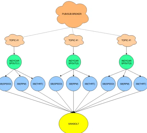
2.3 Application Architecture

Figure 1: Storm topology structure (limited to display three cars)

3

Experiments and Results

3.1 Input data and experimental setup

We run our application on the data logged for the 2017 race held on the Indianapolis Motor Speed-way. For reasons of being private and high-value data to individual racing teams, we had limited access to the data. The telemetry data is available in eRP (enhanced Results Protocol) format, and it’s a subset of the entire telemetry logged throughout the race. In the future, we intend to run our application over the entire data for Indycar 2018. To effectively communicate the behavior of the input data and our results, we limit our view to cars #8,#10 and #11. The data patterns exhibited by the three cars give us plenty of opportunities to detect anomalies and hence, narrow our focus to conduct an in-depth analysis of the results. Figure 1 shows thevehicle_speedattribute for the three cars. The input value of 0 mph points to the start line, pit stops, and the finish line.

We run the application in two modes: sequentialandstreaming. The sequential mode is, as the name suggests, a single-threaded process running on a single machine, while in streaming mode, we run a Storm topology with multiple executors, thus adding parallelism. We also deploy Storm application with a parallelism of 1 to conduct a one-on-one comparison against the batch mode and determine the overhead incurred of running the same task in a distributed mode for the same compute resources, if any. We also run HTM on NuPIC (NUmenta’s Platform for Intelligent Computing) native python library and compare the results.

In sequential mode, we launch anomaly detection on telemetry data as single threaded java process running on just one machine. The set heap size for the execution was 16 gigabytes. Assuming we run one task per executor in the streaming mode, the total number of nodes needed to run our Storm topology is:

Total No. of Tasks

Total Cores available (2)

We deploy the anomaly detection application as a topology comprised ofIndycarSpout, Scalar-MetricBolt, andSinkbolt. In our current implementation, we run anomaly detection on the metrics vehicle_speed,engine_rpmandthrottlecorresponding to each car. Thus, we run one spout and three bolts for every car, the output of which goes to the sink; giving a total of five tasks. Hence, for 33 cars, we have a total of 133 tasks. Since each node consists of 48 cores, we need133₄₈= 3nodes to run our Storm topology in a distributed fashion. The minimum worker heap size set in Apache Storm is 16 gigabytes. To simulate a streaming scenario, we write a parser to process the raw logs and publish the data to the MQTT endpoint. The MQTT broker acts as the communication endpoint between the sensors on the edge and our system, as well as the system and the end-user dashboard. We logically execute our topology structure in the form of a YAML file (yet another markup lan-guage) and launch the application on top of Storm Flux. The finaltopology.yaml launches the appli-cation for anomaly detection for all 33 cars on the metrics vehicle_speed, engine_rpm, and throttle. The following command launches the IndyCar topology:

storm jar Indycar500-1.0-SNAPSHOT.jar org.apache.storm.flux.Flux –remote finaltopol-ogy.yaml

3.2 Execution Latency

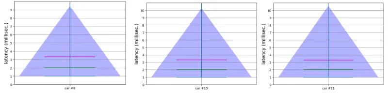
Figure 3 constitutes the violin plots for the execution latency corresponding to cars #8, #10 and #11.

Figure 3: Execution latency for cars #8, #10 and #11

The application, executed multiple times, gave an average execution latency of 3.34 ms for car #8, 3.33 ms for car #10, and 3.27 ms for car #11. There is an initial overhead attributed to the HTM network instantiation and allocation of memory buffers for layers of SDRs on the arrival of the first input, which gradually declines. The spatial and temporal poolers (the layers of the HTM network) register high anomaly scores initially as every record is an anomaly in the beginning, which eventually flattens out as the model learns the pattern. At the start, there are no predictive states; hence, every cell in the mini-columns gets activated, incurring higher time to change their states.

3.3 QoD

that data point. The anomaly score is a float-type value between 0.0 and 1.0, with 0.0 flagged as a normal/expected value and 1.0 flagged as a definite anomaly. The anomaly scores generated subject to parameters used to define the input layers (SP and TM), like learning radius, permanence, threshold, minimum and maximum input value, and more. For an optimized set of such parameters and domain expertise, it is possible to determine a minimum value of the threshold for the anomaly scores where the system triggers an anomaly corresponding to the input data point. For instance, based on the preliminary results, we see that an anomaly score greater than or equal to 0.3 captures all the major fluctuations in the vehicle_speed metric for the cars. In our current implementation, the learning process takes place over the entire course of the race. The fact is evident in figure 4 where the anomaly score (red line) is high whenever we see a sharp change in input metric (blue line). The anomaly score remains comparatively low when the input exhibits a relatively consistent pattern. Alternatively, we can influence the learning range (say limit learning to a fixed number of laps in history) based on a moving average [6].

Figure 4: anomaly scores on vehicle_speed & engine_rpm

Furthermore, we examined the influence of the minimum and maximum value set for a metric on the execution latency and the anomaly scores. We observed that setting a <min., max.> value of <0.0,250.0> for vehicle_speed resulted in higher latency and higher values of anomaly scores than the value <-50.0,300.0>. We know that speed of -50.0 mph makes no sense since a car can either be stationary (vehicle_speed=0 mph) or moving (vehicle_speed > 0 mph). However, we have an appreciable zero data points (vehicle_speed, engine_rpm, throttle, et al. =0.0) in the race telemetry, courtesy of pit stops. Setting minima of 0.0 in a dataset that already contains a plethora of 0.0 results in high values of anomaly scores since that data point is also an extremum. The high latency is a result of activations of columns that are not in the predicted state, thus resulting in activation of every cell of the said column (referred to as boosting).

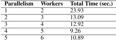
3.4 Sequential vs Streaming mode performance

and three workers (two workers running one executor each ofScalarmetricBoltand one running IndycarSpout), we get a total runtime of 13.09 seconds. We similarly calculate the total runtime for different levels of parallelism and workers as shown in the table.

Parallelism Workers Total Time (sec.)

1 2 23.93

2 3 13.09

3 4 12.92

4 5 9.26

5 6 10.89

To quantify the improvement of running HTM on a streaming framework regarding runtime, we plot the speedup achieved from the table above. The speedup,Sis given by equation (2).T1is the time taken by the batch HTM job, whileTpis the time taken by Storm running with parallelismp. We see the speedup plot in the following figure. The fall in speedup from parallelism of 4 to 5 is attributed to load imbalance.

S= T1

Tp

(3)

Figure 5: Speedup in HTM anomaly detection

3.5 NuPIC Python vs. HTM.java

In this section, we describe the performance nuances between NuPIC’s python and our HTM.java packages in terms of the latency and QoD. The NuPIC python library is the official implementation of HTM by Numenta, while HTM.java is the open-source community-managed implementation of HTM. Since we use HTM.java library in our streaming application, we decided to run anomaly detection on the same dataset and compute node for both libraries and evaluate the results. Table 2 lists the average execution latency (in milliseconds) for the two algorithms for the given cars.

Car # NuPIC python HTM.java

8 3.32 3.34

10 3.03 3.33

11 3.44 3.27

The latency performance of both the libraries is almost the same. In spite of Java being faster than Python, there are ˜30 data points around the 19000th record index, where the queue of the publisher object in HTM gets filled. At the point, memory buffers need to be re-allocated. In these 30 data points, we observe relatively high latencies (500-800 ms), which eventually come back down to 1-2 ms. These outliers affect the average execution latency in HTM.java. In Python, the entire input dataset is passed as a single batch in the form of a CSV file instead of publishing one object at a time as we have done in the Java implementation.

the value of anomaly score fluctuated between 0.0 and 1.0 more evidently and in synchrony with the flow of the input data.

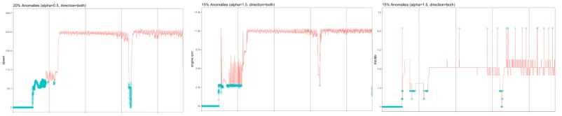
3.6 SH-ESD Test

We show the anomaly detection capability of the Seasonal Hybrid ESD test on the metrics vehi-cle_speed, engine_rpm and throttle for a single car in figure 6.

Figure 6: SH-ESD detection on the three metrics

4

Conclusion

In our paper, we evaluate the choice of using HTM for anomaly detection in a distributed real-time streaming application. We compare HTM with another anomaly detection algorithm, SH-ESD and justify the advantages of the former over the latter. Additionally, we define two metrics that are critical to our application: execution latency and quality of detection (QoD). To develop a useful streaming application, the latency incurred to flag an input as anomalous or usual must be minimal, while the accuracy, i.e., QoD of our application must be high (for obvious reasons!).

We demonstrate the speedup of our distributed application against that of sequential execution on the same dataset and parameters specific to the HTM algorithm. We enumerate the improvements in end-to-end run time for various levels of parallelism in our Storm application. We compare the open-source Java implementation of HTM with the official Numenta managed, NuPIC python. We compare the average execution latencies for similar input parameters and dataset on various cars. Last, we evaluate the performance of the SH-ESD algorithm on the Indycar telemtry. Although faster than HTM on a single node, SH-ESD exhibited poorer QoD and cannot be leveraged to run on a ditributed system.

References

[1] Alexandre Vivmond. Utilizing the htm algorithms for weather forecasting and anomaly detection.Master Thesis, 2015.

[2] A. Lavin and S. Ahmad. Evaluating real-time anomaly detection algorithms – the numenta anomaly bench-mark. pages 38–44, Dec 2015.

[3] Subutai Ahmad, Alexander Lavin, Scott Purdy, and Zuha Agha. Unsupervised real-time anomaly detection for streaming data.Neurocomputing, 06 2017.

[4] Subutai Ahmad and Jeff Hawkins. Properties of sparse distributed representations and their application to hierarchical temporal memory.arXiv preprint arXiv:1503.07469, 2015.

[5] Subutai Ahmad and Jeff Hawkins. How do neurons operate on sparse distributed representations? a math-ematical theory of sparsity, neurons and active dendrites.CoRR, abs/1601.00720, 2016.