Improvement of the Traditional Canny Edge Detection Algorithm by using Combination of Arithmetic Mean Filter, Harmonic Mean Filter and Geometric Mean Filter

(1)

International Journal of Innovative Technology and Exploring Engineering (IJITEE) ISSN: 2278-3075, Volume-9 Issue-2, December 2019



Abstract: Canny Edge Detection Algorithm was very popular on the computer vision area which used to preserve the edges of the image. Due to the defect of the Canny Edge Detection Algorithm like no efficiency on noise removal, some improvement on the Canny Edge Detection Algorithm was done by the researchers. On this paper, a new enhanced Canny Edge Detection Algorithm will be propose which replaces the Gaussian Filter with combination of Arithmetic Mean Filter, Harmonic Mean Filter and Geometric Mean Filter. The replace of Gaussian Filter with combination of Arithmetic Mean Filter, Harmonic Mean Filter and Geometric Mean Filter is to improve the performance of Canny Edge Detection Algorithm on noise removal. A comparison between Canny Edge Detection Algorithm proposed by this paper, Canny Edge Detection Algorithm proposed by (Ilkin, Tafralı, &Sahin, 2017) and traditional Canny Edge Detection Algorithm will be done. The comparison will done by using eight images with different type and size which corrupted by noise. The performance of three algorithms will be determined by using the Peak Signal to Noise Ratio (henceforth, PSNR) value which uses as a quantitative measure. From the result, the Canny Edge Detection proposed by this paper will provide a better performance on noise removal and which will give a better impact on preserve the edges of the images corrupted by noise.

Keywords : Canny Edge Detection, Harmonic Mean Filter, Arithmetic Mean Filter, Geometric Mean Filter, Peak Signal to Noise Ratio

I. INTRODUCTION

E

dges on the image contain a lot of information and detail which are very useful. So the method to preserve the edges of the images were a big challenge. Many researchers pro-posed many different type of edge detection algorithm and the most common algorithm was Canny Edge Detection Algorithm (henceforth, CEDA). Edge detection is a process to finding the sharp discontinuities and locating it.

Although CEDA was common used in the image

Revised Manuscript Received on December 05, 2019.

Ng Kok Soon, Faculty of Information & Communication Technology, Universiti Teknikal Malaysia Melaka, Hang Tuah Jaya, 76100 Durian Tunggal, Melaka, Malaysia.

Zuraida Abal Abas, Faculty of Information & Communication Technology, Universiti Teknikal Malaysia Melaka, Hang Tuah Jaya, 76100 Durian Tunggal, Melaka, Malaysia

Asmala Ahmad, Faculty of Information & Communication Technology, Universiti Teknikal Malaysia Melaka, Hang Tuah Jaya, 76100 Durian Tunggal, Melaka, Malaysia

Hidayah Rahmalan, Faculty of Information & Communication Technology, Universiti Teknikal Malaysia Melaka, Hang Tuah Jaya, 76100 Durian Tunggal, Melaka, Malaysia

processing, but it also got some defects. The first defect is slow processing and cause the CEDA cannot apply on the real time [2]. The second defect was the weak anti-noise ability which mean not function well on the noise removal [12]. So that are a lot of improvement and enhancement done by many researchers. This paper will focus on solving second defect of the CEDA which are replace the Gaussian Filter on the CEDA with the combination of the Arithmetic Mean Filter, Harmonic Mean Filter and Geometric Mean Filter.

In section 2 the previous work done by the researchers, few filtering methods and step of traditional CEDA was discussed. Section 3 gives information about the enhancement of CEDA in this paper and the images and algorithm using for testing. Section 4 gives the result of the implementation of various canny edge detection algorithm on image corrupted with noise. Finally, Section 5 discusses conclusion and section 6 is about the future scope of the work.

II. RELATED WORK A. Previous Work

A comparison between Edge Detection Techniques was done by [5], [6] and [10]. The result shows that the CEDA got a better performance compare with others. So CEDA was widely used on many application or system which related to image processing. Many researchers was propose an improvement or enhancement of the CEDA to solve the defect of CEDA.

The first defect of the traditional CEDA is processing speed. [2] states that the traditional CEDA is a time consuming algorithm and cannot be implemented in real time. So [2] proposes implementing the CEDA based on an FPGA platform to increase the speed of operation. [4] propose perform the image segmentation by taken the output image of the CEDA as the input image. Chan-Vese algorithm will be used on the image segmentation step. [3] proposes combine the Otsu method with maximum entropy method to determine threshold of CEDA. [1] proposes divide whole input image into fixed size of blocks and each blocks of image will undergoes the CEDA individual to increase the processing speed. [7] proposes improve the efficiency of CEDA by using Ant Colony Optimization Algorithm. A new approach was proposed by [13] to improve the CEDA which divides the image into the sub-image and each sub-image will undergoes CEDA individual.

Improvement of the Traditional Canny Edge

Detection Algorithm by using Combination of

Arithmetic Mean Filter, Harmonic Mean Filter

(2)

Mean Filter, Harmonic Mean Filter and Geometric Mean Filter

The second defect of traditional CEDA is the performance of

noise removal. [12] pro-poses using the median filter to replace Gaussian Filter on the filtering step and Frei-Chen algorithm and Ostu-Algorithm will be used to calculate gradient amplitude. Ac-cording [14], Bilateral Filter will replace the Gaussian Filter on CEDA which provide better performance on noise removal. [16] proposes replace the Gaussian Filter with LoG Filter to preserve more detail of the image. Mean Filtering will be used by [11] to enhance the CEDA.

B. Filtering Method

i. ArithmeticMean Filter (henceforth, AMF)

AMF is a Linear Filter and within the window, all the values of pixels will be average. Equation 1 was the equation of the AMF.

(1) Where

= ArithmeticMean = total dataset

= value of dataset

ii. Harmonic Mean Filter (henceforth, HMF)

The true picture of average data will be given by HMF. HMF can be shown mathematically as equation 2.

(2)

Where

= HarmonicMean = total dataset

= value of dataset

iii.Geometric Mean Filter (henceforth, GMF) Almost same as the AMF but GMF lose less detail of the image. Equation of GMF was shows on equation 3.

(3)

Where

= GeometricMean = total dataset

= value of dataset

C. Traditional CEDA Step 1: Filtering

Gaussian Filter (henceforth, GF) was using to filter the noise on the image with smoothing and blurring effect. Besides that, GF also can used to remove the unwanted detail on the image. Equation 4 show the equation of GF.

(4)

= the distancefrom originin the horizontal axis = the distancefrom originin thevertical axis

First derivative of Gx and Gy will be obtained by filtered the image gain from previous step with a Sobel kernel. The filtered process will in both vertical and horizontal direction. Equation 5 and 6 show the way to calculate edge gradient and direction for each pixel from the images.

Gx = horizontal direction Gy = vertical direction

(5)

(6)

Direction of gradient is perpendicular to the edges and is rounded by four angles which represent horizontal, vertical and two diagonal direction.

Step 3: Non-maximum suppression

When the direction and gradient magnitude obtained, unwanted pixels will be remove by scanning the image. Every pixel will be checked if it is a local maximum in its neighborhood in the direction of gradient.

Fig. 1. Example of determine local maximum From Figure 1, the direction of Point A is vertical and on the edge. The gradient direction got the Point B and C which normal to the edge. To verify point A is a local maxi-mum, point A will be checked with point B and C. If point A is not local maximum, it is suppressed, otherwise, next stage will be considered.

Step 4: Hysteresis Thresholding

To differentiate the edges and non-edges, minVal and mxVal will be used. If the intensi-ty gradient of the edges is more than maxVal, then the edges will be edges. If the intensity gradient of the edges is below minVal, then the edges are non-edges and will be discarded. If the intensity gradient is between minVal and mxVal, differentiate of edges are non-edges will based on their connectivity. If the edges are connected to "sure-edges" pixels, they will be classified as part of edges. If not, they will discarded.

Fig. 2. Example of differentiate edge

(3)

[image:3.595.357.490.60.172.2]

Figure 3 shows the flow of traditional CEDA.

Fig. 3. Flow of traditional CEDA III. METHODOLOGY

In this paper, we propose combine the AMF, HMF and GMF to replace the GF when applying the CEDA.

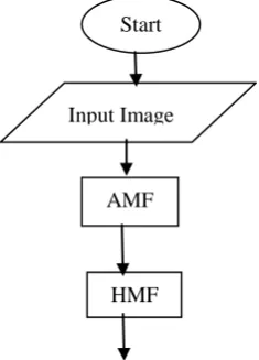
Step 1: Filtering

[image:3.595.77.252.70.411.2]

Combine the AMF, HMF, and GMF to replace the GF. The image will undergoes AMF first to get output image, After that the output image will undergoes HMF and finally the output image get form HMF will undergoes GMF to get a final output image.

[image:3.595.352.501.484.546.2]

Figure 4 shows the flow of combination of AMF, HMF, and GMF.

Fig. 4. Flow of traditional CEDA Step 2: Finding intensity gradient of the image

First derivative of Gx and Gy will be obtained by filtered the image gain from previous step with a Sobel kernel. The filtered process will in both vertical and horizontal direction. Equation 5 and 6 show the way to calculate edge gradient and direction for each pixel from the images.

Gx = horizontal direction Gy = vertical direction

(7)

(8)

Direction of gradient is perpendicular to the edges and is rounded by four angles which represent horizontal, vertical and two diagonal direction.

When the direction and gradient magnitude obtained, unwanted pixels will be remove by scanning the image. Every pixel will be checked if it is a local maximum in its neighborhood in the direction of gradient.

Fig. 5. Example of determine local maximum From Figure 5, the direction of Point A is vertical and on the edge. The gradient direction got the Point B and C which normal to the edge. To verify point A is a local maxi-mum, point A will be checked with point B and C. If point A is not local maximum, it is suppressed, otherwise, next stage will be considered.

To differentiate the edges and non-edges, minVal and mxVal will be used. If the intensity gradient of the edges is more than maxVal, then the edges will be edges. If the intensity gradient of the edges is below minVal, then the edges are non-edges and will be discarded. If the intensity gradient is between minVal and mxVal, differentiate of edges are non-edges will based on their connectivity. If the edges are connected to "sure-edges" pixels, they will be classified as part of edges. If not, they will discarded.

Start

Step 1: Filtering

Step 2: Finding the intensity gradient of the image

End Input Image

Output Image

Start

AMF

HMF

GMF

End Output Image

[image:3.595.103.221.599.763.2]

(4)

Mean Filter, Harmonic Mean Filter and Geometric Mean Filter

Fig. 6. Example of differentiate edge

[image:4.595.305.534.44.426.2]

From the Figure 6, edge A is higher than maxVal so it is "sure-edge". Edge C also consider as valid edge because it connected to edge A. edge B will be discarded because it do not connected to any "sure-edge". So, to get an accurate result, minVal and maxVal play an important role.

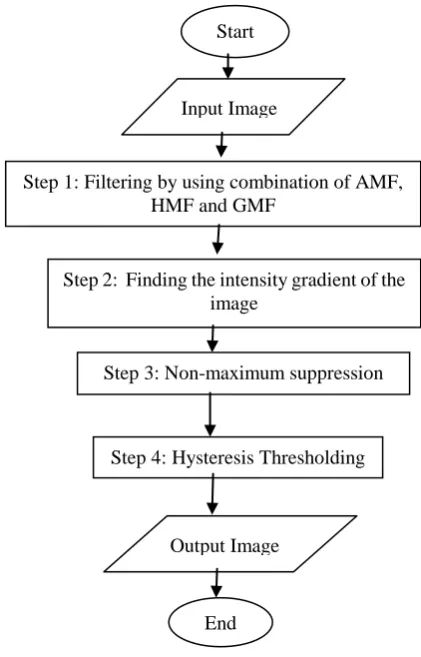
[image:4.595.96.238.53.108.2]

Fig. 7. Flow of enhanced CEDA

Figure 8 show the 4 original pictures get from internet with different size. Then Figure 9 show the pictures which corrupted by noise with amount of noise is 50 and strength of noise also is 50. The images also including Monochromatic (grayscale noise). Figure 10 shows the 4 gray-scale images taken by smart phone with different size. Then Figure 11 shows the gray-scale images corrupted by noise with amount of noise is 50 and strength of noise also is 50. The images also including Monochromatic (grayscale noise). The tool for adding the noise is https://pinetools.com/add-noise-image. The corrupted images and pictures show on Figure 9 and 11. The corrupted images will be used to test the performance of CEDA.

a. .jpg image with dimensions 750 x 536

b. .jpg image with dimensions 623 x 417

c. .jpeg image with dimensions 500 x 310

d. .jpg image with dimensions 736 x 479 Fig. 8. Original Images

c. .jpeg image with dimensions 500 x 310

[image:4.595.65.276.213.542.2]

d. .jpg image with dimensions 736 x 479 Fig. 9. Images from Figure 8 which corrupted by noise

c. .jpg image with dimensions 4608 x 3456

d. .jpg image with dimensions 4608 x 3456 Fig. 10. Original Images taken by smart phone Start

Step 1: Filtering by using combination of AMF, HMF and GMF

Step 2: Finding the intensity gradient of the image

End Input Image

[image:4.595.312.542.457.674.2]

(5)

c. .jpg image with dimensions 4608 x 3456

[image:5.595.47.289.48.311.2]

d. .jpg image with dimensions 4608 x 3456 Fig. 11. Images from Figure 7 which corrupted by noise The images with noise will be undergoes CEDA process to detect the edges of images. The output image will be using to get the performance of the CEDA in term of noise filtering and preserving the edges and details of images. The experiment was carried out with three CEDA which shows at Table 1. All the algorithm are developed by Java code using Netbeans software.

Table 1. CEDA used for the experiment

No Method Propose Year

i Traditional CEDA 1986

ii Enhanced CEDA propose by

[11]

2017

iii Enhanced CEDA propose by this paper

2019

[image:5.595.49.289.426.517.2]

[11] propose using the mean filter to filtering the image before undergoes traditional CEDA. Figure 12 show the flow of enhanced CEDA propose by [11].

Fig. 12. Flow of enhanced CEDA propose by [11] IV. RESULT

Quality of the reconstructed image can be determine by PSNR value. The PSNR value is a quality measurement for the original image and reconstructed image. The higher the PSNR value, the higher the quality of reconstructed image [17].

(9)

(10)

Where r represent the original image and x represent the restored image. Size of image represented by M * N.

Mean Filter

Traditional CEDA process which shows on Figure 2

End

Start

Input Image

[image:5.595.99.242.564.766.2]

(6)

[image:6.595.54.551.60.766.2]

Mean Filter, Harmonic Mean Filter and Geometric Mean Filter

Table 2. . Output Image after implement CEDA on image

Image Original Algorithm Enhanced CEDA propose by [11] Propose Algorithm

a

b

c

d

e

f

g

(7)

[image:7.595.76.522.70.185.2]

Table 3. PSNR value after implement CEDA on image

Image Original Algorithm Enhanced CEDA propose by [11] Propose Algorithm

a 4.28 4.38 4.41

b 6.77 7.10 7.12

c 4.38 4.56 4.57

d 8.04 8.29 8.44

e 4.59 4.11 4.62

f 6.14 5.56 6.20

g 5.72 5.27 5.74

h 6.42 6.42 6.51

Table 2 show the output image obtained after three different CEDA used to preserve the edges of images shown on Figure 9 and 11. Besides that, the PSNR value of output image obtained after CEDA process also provided on Table 3. . From table 2 and 3, we can conclude that the CEDA propose by this paper will give the highest PSNR value which mean better performance on filter the noise and preserve the edges and details of the images. Table 4 will show the Algorithm with the highest PSNR value and their PSNR value.

Table 4. Algorithm with the highest PSNR Image Algorithm with Highest PSNR

Value

PSNR value

9(a) Propose Algorithm 4.41

9(b) Propose Algorithm 7.12

9(c) Propose Algorithm 4.57

9(d) Propose Algorithm 8.44

11(a) Propose Algorithm 4.62

11(b) Propose Algorithm 6.20

11(c) Propose Algorithm 5.74

11(d) Propose Algorithm 6.51

V. CONCLUSION

We present a better CEDA to preserve the edge and details of the images which corrupted by noise. The combination of AMF, HMF, and GMF provide a better filtering result compare with Gaussian Filter. The defect of CEDA is no efficiency on noise removal and the traditional CEDA was using Gaussian Filter. Due to the combination of AMF, HMF, and GMF provide a better filtering result compare with Gaussian Filter, so we replace the Gaussian Filter with the combination of AMF, HMF, and GMF. From the experiment and analysis done, we successful prove that replace the Gaussian Filter with combination of AMF, HMF, and GMF on CEDA will provide a better performance on preserve the edges and details of the images corrupted by noise.

VI. FUTURE SCOPE

This paper can be extended by including various type of noise and test the performance of various CEDA on different type of noise. Besides that, the processing speed of CEDA also can be include in the experiment at future.

ACKNOWLEDGEMENT

Special thanks to Ministry of Education Malaysia for granting

a grant FRGS/2018/FTMK-CACT/F00394 and

FRGS/1/2015/ICT04/FTMK/02/F00286. A special thanks also to University Teknikal Malaysia Melaka.

REFERENCES

1. D. K.Maladakara andH. R.Vanamala, “Design of Improved Canny Edge Detection Algorithm,” Int. J. Softw. Hardw. Res. Eng., vol. 3, no. 8, pp. 33–40, 2015.

2. P. S.Deokar, “Implementation of Canny Edge Detector Algorithm

using FPGA,” Int. J. Innov. Sci. Eng. Technol., vol. 2, no. 6, pp. 1–4, 2015.

3. Y.Wang andJ.Li, “An Improved Canny Algorithm with Adaptive

Threshold Selection,” in MATEC Web of Conferences, 2015, vol. 7, no. 2, pp. 1–7.

4. K. D.Kundapur andA. S. A.S, “An Enhanced Edge Detection

Algorithm,” in Special Issue - 2015 International Journal of Engineering Research & Technology (IJERT), 2015, vol. 3, no. 19, pp. 1–4.

5. S.Kaur andI.Singh, “Comparison between Edge Detection

Techniques,” Int. J. Comput. Appl., vol. 145, no. 15, pp. 15–18, 2016.

6. Ş.Öztürk andB.Akdemir, “Comparison of Edge Detection Algorithms

for Texture Analysis on Glass Production,” Procedia - Soc. Behav. Sci., vol. 195, pp. 2675–2682, 2015.

7. P. D.Rao andS.Rai, “Ant Colony Optimization Algorithm for

Improving Efficiency of Canny Edge Detection Technique for Images,” IJSRSET, vol. 2, no. 6, pp. 350–355, 2016.

8. Nisha andD. R.Khanna, “a Review of Image Restoration Techniques

for Salt-and-Pepper,” Int. J. Adv. Res. Electron. Commun. Eng., vol. 4, no. 2, pp. 2–5, 2015.

9. S.Kaur, “Noise Types and Various Removal Techniques,” Int. J. Adv.

Res. Electron. Commun. Eng., vol. 4, no. 2, pp. 226–230, 2015.

10. S. C.Shekar andD. J.Ravi, “Image Enhancement and Compression

using Edge Detection Technique,” Int. Res. J. Eng. Technol., vol. 4, no. 5, pp. 1013–1017, 2017.

11. Ilkin, S., Tafralı, M., &Sahin, S. (2017). THE ENHANCEMENT OF

CANNY EDGE DETECTION ALGORITHM USING PREWITT ROBERT AND SOBEL KERNELS. In International Conference on Engineering Technologies.

12. Y.Feng, J.Zhang, andS.Wang, “A new edge detection algorithm based

on Canny idea,” in AIP Conference Proceedings, 2017, vol. 1890, no. 2017.

13. M. H.Shokhan, “AN EFFICIENT APPROACH FOR IMPROVING

CANNY EDGE DETECTION ALGORITHM,” Int. J. Adv. Eng. Technol., vol. 7, no. 1, pp. 59–65, 2014.

14. I.Fawwaz, M.Zarlis, Suherman, andR. F.Rahmat, “The edge detection

enhancement on satellite image using bilateral filter,” in IOP Conference Series: Materials Science and Engineering, 2018, vol. 308, no. 1.

15. J.Cao, L.Chen, M.Wang, andY.Tian, “Implementing a Parallel Image

Edge Detection Algorithm Based on the Otsu-Canny Operator on the Hadoop Platform,” Comput. Intell. Neurosci., vol. 2018, 2018.

16. L.Xuan andZ.Hong, “An improved canny edge detection algorithm for

Detecting Brain Tumors in MRI Images,” Proc. IEEE Int. Conf. Softw. Eng. Serv. Sci. ICSESS, vol. 2017-Novem, pp. 275–278, 2018.

17. R.Kaur andR.Maini, “Performance Evaluation and Comparative

Analysis of Different Filters for Noise Reduction,” Int. J. Image, Graph. Signal Process., vol. 8, no. 7, pp. 9–21, 2016.

18. R.Mehra, “Estimation of the Image Quality under Different

(8)

Mean Filter, Harmonic Mean Filter and Geometric Mean Filter

AUTHORS PROFILE

Ng Kok Soon is a master student in Faculty

of Information and Communication

Technology, University Teknikal Malaysia Melaka. He has received his BSc. Computer Science (Database Management)

from University Teknikal Malaysia

Melaka.

Zuraida Abal Abas is Associate Professor

in Faculty of Information and

Communication Technology, University Teknikal Malaysia Melaka. She has received her BSc. Industrial Mathematics from University Teknologi Malaysia (UTM). Besides that, she also received her MSc. Operational Research from London School of Economics, UK and received her Doctor of Mathematics from University Teknologi Malaysia (UTM). The field of specialization for Dr Zuraida Abal Abas is operational research and mathematics.

Asmala Ahmad is Associate Professor in Faculty of Information and Communication Technology, University Teknikal Malaysia Melaka. He has received his BAppSc.

Geophysics from University Sains

Malaysia (USM). Besides that, he also received his MSc. Remote Sensing from University Teknologi Malaysia (UTM) and received his PhD. Applied Mathematics from University of Sheffield, UK. The field of specialization for Dr Asmala Ahmad is remote sensing, image processing and applied mathematics.

Hidayah Rahmalan is senior lecturer in Faculty of Information and Communication Technology, University Teknikal Malaysia Melaka. She has received her BSc. In

Computer Science from University

Teknologi Malaysia (UTM). Besides that, she also received her MSc. Computer

Science from University Teknologi