The economic and energy impacts of a UK export shock: comparing alternative modelling approaches

This is a repository copy of The economic and energy impacts of a UK export shock: comparing alternative modelling approaches.

White Rose Research Online URL for this paper: http://eprints.whiterose.ac.uk/151335/

Version: Published Version

Monograph:

Allan, Grant, Barrett, John, Brockway, Paul et al. (7 more authors) (2019) The economic and energy impacts of a UK export shock: comparing alternative modelling approaches. Working Paper. UKERC , UK.

[email protected] https://eprints.whiterose.ac.uk/

Reuse

Items deposited in White Rose Research Online are protected by copyright, with all rights reserved unless indicated otherwise. They may be downloaded and/or printed for private study, or other acts as permitted by national copyright laws. The publisher or other rights holders may allow further reproduction and re-use of the full text version. This is indicated by the licence information on the White Rose Research Online record for the item.

Takedown

If you consider content in White Rose Research Online to be in breach of UK law, please notify us by

1

The economic and energy impacts of a UK

export shock: comparing alternative modelling

approaches

Grant Allan

_{, John Barrett}

_{, Paul Brockway}

_{, Marco Sakai}

_{, Lukas Hardt}

_{, Peter}

G. McGregor

, Andrew G. Ross

, Graeme Roy

, J. Kim Swales

, and Karen Turner

a _{Fraser of Allander Institute, Department of Economics, Strathclyde Business School,}

University of Strathclyde

b _{Sustainability Research Institute, School of Earth and Environment, University of Leeds} c _{Department of Environment and Geography, University of York}

d _{Centre for Energy Policy, University of Strathclyde}

2

Introduction to UKERC

The UK Energy Research Centre (UKERC) carries out world-class, interdisciplinary research into sustainable future energy systems.

It is a focal point of UK energy research and a gateway between the UK and the international energy research communities.

Our whole systems research informs UK policy development and research strategy. UKERC is funded by the UK Research and Innovation Energy Programme.

For information please visit: www.ukerc.ac.uk Follow us on Twitter @UKERCHQ

Acknowledgements

This research was undertaken at the Fraser of Allander Institute at the University of Strathclyde, the Sustainability Research Institute at the University of Leeds, Department of Environment and Geography at the University of York, and Centre for Energy Policy at the University of Strathclyde as part of the research programme of the UK Energy Research Centre, supported by the UK Research Councils under EPSRC award EP/L024756/1. This work draws upon analysis given in Ross et al. (2018a,b).

3

Contents

List of Tables 5

List of Figures 5

Abstract 6

1 Introduction 7

2 Comparing CGE and ME Energy-Economy Models 9

2.1 Theoretical basis 9

2.1.1 Brief overview of two approaches to macroeconomic theory ... 9

2.1.2 Labour market ... 11

2.1.3 Capital market and crowding out ... 12

2.2 Model specification 2.2.1 Sectoral structure and energy ... 12

2.2.2 Treatment of time ... 13

2.2.3 Expectations formation ... 14

2.3 Model parameterisation 2.4 Model solution 2.5 Model simulation 3 Simulation strategy 3.1 Implementing the export shock in UK-ENVI and MARCO-3.2 Assumptions about fiscal policy 4 Model and data 4.1 UK-ENVI model 4.1.1 Consumption and trade ... 18

4.1.2 Production and investment ... 19

4.1.3 The labour market ... 20

4.1.4 Government ... 21

4.1.5 Dataset and income disaggregation and energy use ... 22

4.2 MARCO-UK model 4.2.1 GDP and aggregate demand ... 23

4

4.2.3 Production inputs: labour, capital and useful exergy... 25

4.2.4 Sectoral structure ... 27

4.2.5 Energy use, energy efficiency and CO2 emissions ... 28

4.2.6 Prices and money ... 29

4.2.7 Data sources and model parameterisation ... 32

5 Simulation results 5.1 UK-ENVI simulation results 5.1.1 Long-run results ... 34

5.1.2 Short-run results ... 36

5.1.3 Energy results ... 36

5.1.4 Sectoral results ... 37

5.1.5 Household results ... 37

5.1.6 Time path adjustments ... 37

5.2 MARCO-UK simulation results 5.2.1 Long-term impacts ... 39

5.2.2 Adjustment dynamics ... 43

5.2.3 Energy and emissions results ... 44 6 UK-ENVI and MARCO-UK simulation results compared

6.1 Long-run effects on GDP and employment 6.2 Short-run effects on GDP and employment 6.3 Price effects

6.4 Energy and emission effects 49

6.5 Policy implications 7 Summary and Conclusion References

MARCO-5

List of Tables

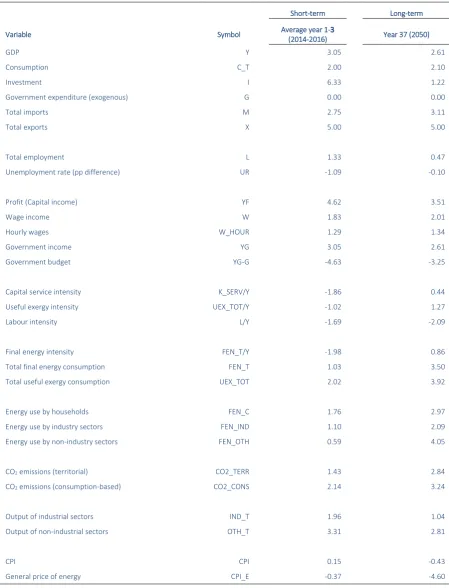
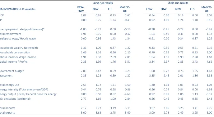
Table 1: Short and long-run effects of a 5% increase in international exports in UK-ENVI. % changes from base year. ... 35 Table 2: Short- and long-term effects of a 5% increase in international exports for some key variables in the MARCO-UK model. Results are presented as % deviation from the baseline scenario, with the exception of the unemployment rate which is presented as percentage point difference in the rate between the export scenario and baseline scenario. ... 40 Table 3: UK-ENVI and MARCO-UK simulation results compared. Short and Long-run effects of a 5% increase in international exports. (Results reported as % changes from base year/ baseline scenario.) ... 46

List of Figures

Figure 1: The structure of consumption in UK-ENVI ... 19 Figure 2: The structure of production in UK-ENVI ... 19 Figure 3: Long-run effects on output, employment, and energy use by individual sectors of a 5% increase in international exports, BRW closure. % changes from base year. ... 38 Figure 4: Long-run effects on household quintiles of a 5% increase in international exports, BRW closure. % changes from base year. ... 38 Figure 5: Aggregate transition path for GDP, employment, and total energy use of a 5% increase in international exports. % changes from base year. ... 39 Figure 6: Change in aggregate demand components in MARCO-UK in response to a 5%

increase in exports applied from 2014. Absolute deviation from baseline scenario in million £. ... 41 Figure 7: Change in aggregate demand components in MARCO-UK in response to a 5%

6

Abstract

Achieving the targets for reducing greenhouse gas emissions set out in the UK Climate Change Act will require a significant transformation in the UK's energy system. At the same time, the government is pursuing a new UK Industrial Strategy, which aims to improve labour productivity, create high-quality jobs and boost exports across the UK. The economic and the energy systems in the UK are tightly linked and so policies adopted in one area will produce spillover effects to the other. To achieve the objectives set out in the two strategies it is therefore vital to understand how the policies in the energy system will affect economic development and vice versa. This study seeks to contribute to this by investigating how an increase in exports (a key pillar in the UK Industrial Strategy) could impact energy- and industrial policy. We address this question by systematically comparing the results of two types of energy-economy models of the UK, a computable general equilibrium model and a macroeconometric model. In terms of the implications of a successful export promotion strategy, the models agree that there is likely to be a beneficial impact on the economy, but an adverse impact on CO2 emissions and energy intensity. This reveals the extent of any policy

adjustment that would be required to maintain a given level of emissions and serves to emphasise the need to complement UK industrial policies with appropriate action on energy use and carbon emissions to meet statutory carbon targets set by the Climate Change Act (2008). Our second main conclusion is that there are advantages to having a diverse mix, or portfolio, of energy-economy models with each having comparative advantages depending on: prevailing circumstances (including the state of the economy); the time-period of interest and the nature of the policy question being addressed.

Key words: energy policy, industrial strategy, trade policy, energy-economy modelling, climate policy

7

1

Introduction

Achieving the targets for reducing greenhouse gas (GHG) emissions set out in the UK Climate Change Act will require a significant transformation in UK energy system. The UK

achieving its climate change targets is set out in the Clean Growth Strategy (HM Government, 2017a). As part of the 2032 pathway set out in the strategy, the UK government aims to reduce the GHG emissions intensity of the UK economy by 5% each year until 2032 and improve the energy productivity of business by 20% by 2030. Overall, the government expects that the 2032 pathway will reduce final energy consumption by 13% compared to baseline projections, which would amount to an approximate reduction of 11% compared to 2016.

At the same time, the government is pursuing an Industrial Strategy with the aim of improving labour productivity, creating well-paid and high quality jobs and increasing economic growth across all regions of the UK (HM Government, 2017b).

The economic and the energy systems in the UK are tightly linked and so the policies adopted in one area will produce spillover effects to the other (see e.g. Ross et al. 2018a; Royston et al., 2018). This interaction could produce potential synergies, but also possibly hinder efforts in each policy area. To achieve the objectives set out in the two strategies, it is therefore vital to understand how the suggested policies in the climate and energy field will impact

economic development and vice versa.

This study seeks to contribute to this understanding by investigating how an increase in exports could impact emissions, and other socio-economic variables in the UK. A central interest in the present paper is therefore on the incremental change in emissions that is likely to arise from export policy actions alone. This identifies the potential additional challenge

G

policy. As in Ross et al. (2018a), we focus on an increase in exports, because

G Industrial Strategy, as part of the ambition to be

G B (HM Government, 2017b). A

be a key goal, precise policies or quantifiable measures are not explicitly stated1_{. Accordingly,}

for now we proxy the impact of a successful trade-enhancing policy by an exogenous (and costless) 5% increase, above the baseline, in international export demands across all sectors of the economy. This augments the analysis in Ross et al (2018a) by providing a systematic comparison with an ME model to highlight the differences and similarities between the approaches.

Secondly, to add further insight, we address this question by comparing and discussing the results of two very different types of energy-economy models. Currently, two dominant approaches to the system-wide analyses that seek to capture the interdependence of the economic and energy sub-systems are computable general equilibrium (CGE) and

macroeconometric (ME) models. Both types of models are widely employed by governments, international agencies and research organisations, academics and private sector

consultancies for the analysis of economic and/or energy policies and other disturbance to

1 _{A UK E “ HM G}

8

the economic and/or energy sub-systems (see e.g. European Comission, 2016; HMRC, 2013; and Scottish Government 2016 for CGE models, and e.g. Dagoumas & Barker 2010; European Commission 2015 and OBR 2015 for applications of ME model).

The applications of these models span a wide range of energy and economic policies. For example, Allan et al., (2007) analyse the impacts of increased efficiency in the industrial use of energy. Figus et al. (2017) identify the impacts of energy efficiency programmes on households. Lecca et al. (2014a) identify total energy rebound effects of improvements in household energy efficiency. The European Commission (2015) analyses policies directed at the promotion of energy efficiency in production or consumption. Ekins et al. (2012) consider the imposition of environmental and other taxes, and Ross et al. (2018a,c,e) consider the impact of other fiscal and industrial policy initiatives.

Given that the interdependence of the energy and economic sub-systems is central to these models, they are well suited to focus on the spillover effects both from economic policies to the energy system and vice versa. This interdependence is often crucial to an in-depth understanding of any given disturbance. For example, the likely impact of energy efficiency policies are transmitted, in part, through induced relative price changes and wider economic

(Hanley et al. 2009).

Assessing the impact of an increase in exports on energy use, for example, is strongly

dependent on the economic assumptions and type of model that is used. The formulation of policy can therefore benefit from taking into account the results of both ME and CGE models, exploiting their complementary strengths. For example, this is routinely done in the provision of evidence to the European Commission (e.g. European Commission 2015). Despite the benefits that the comparison of CGE and ME models can bring, it has rarely been applied to policy making in the UK.

The comparison of the two model types in this study therefore serves two important

functions. First, it allows us to provide more robust evidence as it takes into account some of the uncertainty that is associated with the structure of any single model. Second, it also allows us to discuss the comparative strengths and weaknesses of the two modelling

approaches. As a result, we hope that this study will be a useful resource to the research and policy community by enhancing the understanding of both modelling approaches and how they can be used together.

While there is a very wide range of both CGE and ME energy-economy models, we focus here on the two models that have been used for analysis within the UK Energy Research Centre (UKERC) research programme; namely UK-ENVI, a computable general equilibrium economy-energy- environment model of the UK, and the UK MAcroeconometric and Resource

COnsumption (MARCO-UK) model, a ME energy-economy model of the UK (Sakai et al. 2019). We set up the UK-ENVI and MARCO-UK models in an analogous way that allows for a

systematic comparison of the system-wide impacts of a demand-side disturbance, an exogenous increase in exports, across the two models. However, when making model comparisons we emphasise where their characteristics are representative of the wider class of ME and CGE models (and also where they are not), so that our analysis has relevance beyond the narrow comparison of these two specific models.

9

some instances in the underlying visions of the UK macro-economy that are embodied in both models, since these inform to a degree the simulation properties of the models in a way that is perhaps not always obvious to non-modellers. We outline differences between the model types in terms of model: theoretical basis; specification; parameterisation; solution and simulation. In Section 3 we set out our modelling strategy, which seeks to ensure that the impact of a successful UK export promotion strategy is simulated in a similar way in both models to facilitate comparison. Section 4 outlines the structure of both models and explains how they are parameterised (and the data required to facilitate this process). In Section 5 we summarise the simulation results from each model initially separately, then compare them in some detail, drawing attention to similarities and differences in Section 6. Section 7 provides brief conclusions.

2

Comparing CGE and

Energy-Economy Models

There is considerable variability even among CGE and ME models, but each approach has some fairly general distinguishing characteristics. In this section, we set out a brief

comparison of the versions of ME and CGE models that have been used within the UKERC consortium to explore energy-economy issues.

2.1

Theoretical basis

2.1.1

Brief overview of two approaches to macroeconomic theory

It is important to begin with an appreciation of the underlying vision of the UK macro-economy embodied within MEs and CGEs. UK-ENVI is a CGE model drawing on neoclassical economic theory. Archetypal CGE models are developed from well-specified, micro-economic theory in which behavioural relationships are derived from optimising agents and in which

H

these assumptions are often relaxed in the current generation of CGE models (including UK-ENVI) to allow for labour market imperfections and involuntary unemployment, which implies

Partridge & Rickman, 2010). CGEs have typically been regarded as reflecting an ultra-neoclassical view of the world in which demand may not matter much (if at all) and supply influences are expected to dominate in terms of affecting the aggregate real economy. However, in UK-ENVI, both demand and supply typically matter for the determination of output and employment.

CGE models rely strongly on theoretical assumptions with regard to the behavioural functions and also assume that the economy as a whole is in equilibrium in the base year. On the one hand, these assumptions allow the construction of detailed models without large amounts of historical time-series data, as many parameters in the model can be derived from the

calibration to a single base year (although it should be noted that some parameters in CGE models are also estimated econometrically). In addition, the stronger alignment with

economic theory can provide CGEs with an advantage in terms of interpreting model results.

O CGE

UK-10

ENVI

curtail elements of endogeneity to allow tracking the source of results that initially appear surprising; incremental model augmentation, and sensitivity analysis (with respect to behavioural functions as well as parameter values). Traditionally, most CGE models were static in nature, but increasingly they incorporate dynamics. UK-ENVI is a dynamic model that generates multiperiod simulations, which track the adjustment paths of all endogenous variables in the model. Accordingly, it can be used directly to compare entire adjustment paths, as well as, of course, impact and long-run effects, with dynamic ME models

MARCO-UK is a ME model based (as is common) on post-Keynesian economic theory, where agent behaviour is not based on optimisation but is instead determined from econometric equations based on historical data. The economy is conceptualised as a non-equilibrium system in the sense that markets are often not efficient and that prices and quantities do not adjust to optimal, market-clearing levels (Barker et al. 2012; Lavoie 2014a). Instead, post-Keynesians consider that prices are set by firms using some form of mark-up pricing, although it is acknowledged that the interplay of supply and demand can impact prices in some

markets (Lavoie 2014b). It is assumed that in most circumstances not all resources are optimally used and that spare capacity exists in the economy, which allows economic growth to be demand led both in the short and long run (Fontana & Sawyer 2016). In the short run, production adjusts to increased demand through the increase in the utilisation of capacity, while in the long run the total capacity of the economy adjusts to demand through increased levels of investment (Taylor et al. 2016). As a result, economic production is not constrained by supply-side factors in the MARCO-UK model. Post-Keynesian theory recognises that supply-side factors, especially insufficient labour supply, can constrain production in unusual circumstances. Such constraints are not explicitly built into the MARCO-UK model, but we take them into account by rejecting any scenarios in which employment outstrips the available labour force2_.

It should also be noted, that the theoretical assumptions underlying CGE and ME models are often contested; for example, there exist conflicting theories of transactor behaviour

depending on circumstances. The modeller

model behaviour (one motivation for the use of a range of UK-ENVI configurations). So, for example, behavioural economists have found evidence of significant and systematic

deviations from rationality that w

behavioural functions. The post-Keynesian theory underlying ME models generally rejects neoclassical microeconomic assumptions describing, rational, utility or profit-maximising agents and also suggest that macroeconomic dynamics cannot be derived solely from definitions of microeconomic behaviour (Lavoie 2014, p.17). Instead ME models rely on behavioural equations that are statistically estimated from historic time-series data. The specification such equations is not only based on economic theory but is also influenced by considerations of statistical significance and data availability, a practice that is sometimes being criticised as being ad hoc. In addition, the use of statistics and historical time series implies the significant assumption that statistical relationships identified in past data are also relevant in the future. This assumption constitutes an important source of uncertainty for ME

2 _{Employment never exceeded the available labour force in any scenario conducted with the MARCO-UK model for this study}

11

model projections into the future, which increases with distance from the current time. This is a challenge inherent to all empirical modelling.

The underlying macroeconomic vision in any model has a significant impact on its properties and the predicted impact of different policy interventions. Two key areas of divergence are the labour and the capital market, which are discussed below.

2.1.2

Labour market

Under limiting neoclassical assumptions, it is assumed that wages always adjust to ensure full employment and the optimal use of all available labour. One configuration of the labour market treatment in UK-ENVI corresponds rather closely to this neoclassical extreme, namely that with Exogenous Labour Supply (ELS), in which employment is fixed. However, UK-ENVI is atypical of CGEs in general in that it seeks to accommodate a range of alternative visions of the labour market and the macro-economy on the grounds that, in general, the evidence does not provide compelling support for any one vision, although it clearly favours some visions over others.

Three further characterisations of the labour market are captured within UK-ENVI. The default version of the model incorporates a wage curve or bargained real wage function (BRW). The BRW version of UK-ENVI is associated with a less markedly neoclassical

macroeconomic perspective than ELS, because it relaxes the strict labour supply constraint associated with ELS, so that demand plays a greater role in determining economic activity. Furthermore, we allow for fixed nominal (FNW) or real wages (FRW), which some would argue might better characterise the behaviour of the UK economy over the last decade. These variants of UK-ENVI emulate the behaviour of Keynesian models over the long run for demand disturbances, because they impact solely on quantities, with no impact on wages or prices. As will become clear, however, within UK-ENVI even fix-wage models are subject to supply constraints in the short run due to the fixity of capital stocks.

In fact, the very widespread support for the empirical relevance of wage curves has led us typically to adopt the BRW configuration of the labour market as our default. UK wage behaviour over the last decade does, however, suggest the merit of seriously considering the impact of fix-wage models (FNW and FRW). These may ultimately prove to

passed since the onset of the Great Recession, that deviation has been very long lasting. We do not believe that the empirical evidence supports the ELS model, but it serves as a useful benchmark of a continuous full-employment model that characterises many national CGE models.

12

turn determined by demand for labour and unemployment. The determination of wages in the MARCO-UK model is therefore not dissimilar to the bargained real wage function employed in UK-ENVI.

2.1.3

Capital market and crowding out

A second feature that is often discussed as a key difference between CGE and ME models is the treatment of capital markets and the crowding out of investment (Pollitt & Mercure 2018). However, this difference is not relevant for our current study because neither UK-ENVI nor MARCO-UK feature detailed treatments of capital markets.

As is common in CGEs, UK-ENVI has no financial sector, and the interest rate is typically exogenous. While financial sectors can be incorporated into CGEs, this is comparatively unusual. The exogeneity of the interest rate is a simplification that is strictly only valid in circumstances where the Central Bank is committed to maintaining it at that level, or where there is a liquidity trap, with interest rates are so low that market participants expect them to rise (and bond prices to fall) and prefer to hold cash (rather than bonds). This may be a

UK H

A

UK-ENVI as configured here; any crowding out that does occur is attributable solely to supply-side constraints.

Similarly, the treatment of the financial sector in the current version of MARCO-UK is limited. The link between the financial and the real economy is largely implicit and relies on the assumption that investment is not constrained by the financial markets. This assumption is not uncommon in ME models (Pollitt & Mercure 2018). MARCO-UK does feature some representation of the money supply and interest rates that determines the general price level. However, the econometric equations estimated for the model assign those monetary variables only a very limited influence on the real economy.

In the wake of the financial crisis the close link between the financial system and the real economy has received increasing attention and the lack of financial sector representation in both CGE and ME models used for economy-environment analysis has attracted criticism (Pollitt & Mercure 2018; Rezai & Stagl 2016). This lack of adequate financial representation is a limitation of both the models employed in this study and should be kept in mind when interpreting the results.

The development of ME and CGE models can typically be regarded as occurring in four main stages: specification; parameterisation; solution and simulation. We consider each stage in turn and discuss the differences among modelling approaches.

2.2

Model specification

The specification of system-wide models must in part reflect the purposes of the model and also the vision of the economic and here the energy system that underlies it.

13

The choice of model structure can significantly affect results. In the present case, it is essential to choose a structure that allows the capture of energy-economy system

interdependencies; both UK-ENVI and MARCO-UK do that, though in rather different ways. The different structures, of course, constrain the kinds of policy questions that can be addressed in each model.

In the present application, UK-ENVI contains 30 sectors, but the precise number and definition of sectors can be varied depending on the question of interest, with full sectoral disaggregation at 94 sectors following the UK disaggregation of economic accounts. The energy system is represented by energy-producing sectors that produce energy as an input into the production of other sectors.

Energy is treated in UK-ENVI as an intermediate input in the sectoral production hierarchy, which has a KLEM (capital-labour-energy- materials) structure. However, the efficiency of energy (and indeed other inputs) can be varied (typically exogenously). The analysis of such changes in energy efficiency in production (e.g. Allan et al., 2007) and in consumption (e.g. Lecca et al., 2014a; Figus et al., 2017) underlies system-wide analyses of rebound effects (e.g. Turner 2009).3 _{Energy demands within each sector, like the demands for labour and capital,}

are derived demands, and domestic energy prices are typically determined by the interaction of the sectors that demand energy and those that supply it (and exogenous external prices). The current version of MARCO-UK is highly aggregated. The overall dynamics of output, employment and capital stocks are determined at the aggregate level of the whole economy. However, the aggregate output is then broken down into two sectors, an industrial and a non-industrial sector, and final energy consumption is determined at this disaggregated level. The nature of ME models as a system of simultaneous econometric equations makes it a challenging task to increase the number of sectors as the complexity of the model increases quickly, which can make it difficult to achieve stable and coherent model behaviours. However, further disaggregation is planned in future versions of MARCO-UK.

The treatment of energy is a key innovative feature of MARCO-UK. It is the first ME model that explicitly includes useful exergy as a production factor. Useful exergy represents the energy that is actually used in the economy, such as the movement of a car or the light emitted by a light bulb. It is the expression of energy use that is closest to the total use of energy services but can still be measured in energy units (Sousa et al. 2017). It has been shown that useful exergy is more closely related to measures of economic output than other measures of energy use (Ayres & Warr 2005; Santos et al. 2016). Useful exergy use is then linked to the use of final energy carriers via an endogenous efficiency variable, representing the technical transformation efficiency from final energy to useful exergy. Drawing on theory developed by Ayres et al. (2003) this efficiency is an important influence on the evolution of the UK economy in the MARCO-UK model (Sakai et al. 2019).

2.2.2

Treatment of time

CGE models often make a conceptual distinction between two time periods. These time periods include the short run, which denotes an equilibrium with fixed capital stocks, and the long run, which denotes the point in time where capital stocks in each sector are fully

14

adjusted to their desired levels.4 _{UK-ENVI can be used in comparative static mode to}

determine short-run and long-run equilibria, but it is typically run in full dynamic mode, in which the adjustment paths from short- to long-run equilibria are tracked. This traces the consequences of any induced changes in investment expenditure on sectoral capital stocks and productive capacity. A stimulus to demand, for example, tends to increase rental rates (profits) and so stimulate investment expenditures. However, this leads to increases in capital stocks and production, which ultimately lowers profitability to normal levels again, but with capacity permanently increased.

ME models, such as MARCO-UK, do not make such a conceptual distinction. MARCO-UK does not optimise any variable and hence the model does not feature an equilibrium produced by the optimising behaviour of transactors and the adjustment of prices at any point in time (although it is assumed that aggregate supply is equal to aggregate demand in every time period according to definitions given by the System of National Accounts). Instead, every time period (one year) is treated the same and the model is solved for each year based on the econometric equations and current and previous values of the model variables. This means that the model variables are continuously changing, generally producing a growing economy. The growth paths of the economy in the model are, in most circumstances, smooth and stable. However, if shocks are applied to the model, such as the export shock applied in our study, the model often shows a period of less stable, fluctuating dynamics, before it settles again unto a stable growth trajectory. Stable trajectories in ME models are also

confusion with the very different equilibria produced by CGE models. Overall MARCO-UK covers the time period from 1971 to 2050, with 1971-2013 as the time period over which the econometric equations are fitted, and 2014-2050 presenting a forward projection of the model.

2.2.3

Expectations formation

MARCO-UK assumes that expectations are myopic. The version of UK-ENVI used in this study also relies on myopic assumptions to facilitate better comparability of model results. This means that the group of agents in the models make decisions only based on the current values of model variables) without looking forward into the future. This is a common

assumption in post-Keynesian economic theory, but it represents a significant deviation from the ultra-rational neoclassical specification, characterised by intertemporal optimisation of households (determining consumption) and firms (investment) under perfect foresight (or rational expectations in the stochastic case). Although not implemented in this study, UK-ENVI can be run under perfect foresight assumptions, with forward-looking consumption and investment behaviour, as well as under myopic assumptions (Lecca et al, 2013). This typically has an impact on time paths of adjustment, but not on long-run results. This option has the advantage of identifying the consequences of eliminating the systematic errors associated with transactor groups that have myopic expectations and allowing an analysis of alternative expectations formation assumptions.

4 _{The definition of the short run captures the idea that it takes time for investment expenditures to augment the capital}

15

2.3

Model parameterisation

UK-ENVI, like many CGEs, is calibrated to a base year Social Accounting Matrix (SAM)5 _{that is}

constructed around data from UK National Accounts. Given the values of certain key parameters (e.g. substitution and demand elasticities, which may themselves be estimated econometrically), the remaining parameters are determined by reconciling model equations with the SAM database. In effect, the strong theoretical assumptions on agent behaviours and the assumption that the economy is in equilibrium in the base year allows the

construction of a very detailed model, without the need for large amounts of time series data. It also aids the interpretation of the model results. Econometric estimation of full CGEs has not yet proved feasible, given the huge data requirements and technical difficulties estimating such large systems.

MARCO-UK, in line with other ME models, contains two types of equations (identities and econometric equations) with each type accounting for about half the number of equations. While identities are generally derived from accounting relationships, econometric equations are parameterised using econometric methods drawing on time series data. The econometric estimation of the MARCO-UK model equations is built on a data set containing time-series of more than 50 variables covering the years 1971 to 2013. This use of time series data to check on model performance is a major strength of ME models (and also means that they more readily facilitate forecasting). It also allows for the underlying behavioural (and other) assumptions in the model to be tested and adapted in line with empirical results, although this trait is not unique to ME models. However, the data intensity of the ME method also presents constraints on the complexity of the models that can be developed and can make it more difficult to interpret model results.

2.4

Model solution

While the non-linearity of CGEs had at one point appeared to present a major technical hurdle, their solution is now routine. UK-ENVI is coded in GAMS and is solved using CONOPT/MINOS (both general purpose nonlinear programming solvers).

The MARCO-UK model consists of a system of simultaneous, linear equations. It is

dynamically solved for each time period using the Gauss-Seidel iterative method included in the EViews econometric software (Startz, 2015).

2.5

Model simulation

MARCO-UK can be used for both ex-post and ex-ante dynamic simulation. However, in the present exercise, as we explain in the next section of the paper, we use both MARCO-UK and UK-ENVI to isolate the ex-ante impact of a simple stimulus to exports so that we can directly compare model results in as straightforward a manner as possible.

16

Currently, neither MARCO-UK nor UK-ENVI are used for forecasting. In principle, CGEs could be used for this purpose, but in practice rarely are. ME models are more suited to develop short-term forecasts.

3

Simulation strategy

We use a simulation of both models to provide a systematic comparison of the system-wide impacts of a demand side disturbance, an exogenous increase in exports, across the two models (model specifications are given in Section 4).

We limit the current analysis to a demand-side disturbance because we want to focus on the comparison of the two models without adding the further complication of multiple scenarios. However, in the future we seek to provide additional comparisons where we shall also

consider the implications of supply-side disturbances such as labour productivity

improvements and increases in energy efficiency in both production and consumption. This will provide a more complete overview of the two models.

3.1

Implementing the export shock in UK-ENVI and

MARCO-To simulate the impact of an export shock we apply a 5% increase in exports to both models and, for each model, obtain the economic impacts by comparing the results of the scenario

W UK-ENVI and MARCO-UK

models up in a similar way, but the structures of the models mean that the scenario has to be implemented in different ways.

The UK-ENVI model is assumed to be in equilibrium calibrated to the base year, so that the baseline scenario simply recreates the baseline values over time. Given the adoption of myopic expectations here, the stimulus to exports is, of course, unanticipated. A permanent export shock, equivalent to 5% of exports in the base year, is then introduced to the model. In UK-ENVI, the shock is implemented by adding the exogenous shock on top of the

endogenously calculated exports in the model in every single year. The resultant stimulus to demand typically puts upward pressure on prices, and this loss of competitiveness can reduce the endogenous component of exports calculated in the model. This means that, depending on the treatment of the labour market, total exports (including endogenous component and exogenous shock), might not increase by 5%. To observe the adjustment of all the economic variables through time, simulations are run for 50 years, the adjustment period to the long run varies but is typically complete within 7-12 years.

17

3.2

Assumptions about fiscal policy

We make the assumptions about fiscal policy as similar as possible in the two models, although some limits are imposed by the different structure. For fiscal policy in UK-ENVI we simply assume that government expenditure is fixed in real terms. In the case of an

expansionary response to the export stimulus, this implies that additional government revenues are simply being accumulated, for example, to retire debt (which has no further feedback because of our monetary policy assumptions). However, we do indicate the likely consequences of recycling the additional tax revenues into current government spending (which, for simplicity we assume to have no supply-side impacts) within UK-ENVI, to give some idea of the quantitative importance of this difference in model set-up, which we report in Ross et al. (2018a). In MARCO-UK, government expenditure is exogenous and is simply kept the same in the baseline and export shock scenarios. The current version of MARCO-UK does not feature a detailed representation of taxes and other government revenues. Instead, it is simply assumed that government income increases in proportion with GDP. The

differences in the treatment of government income can lead to differences in the wider results as it determines how much of any extra income generated from the export shock is recycled into further spending and economic activity. However, a sensitivity analysis

conducted for the MARCO-UK model suggests that the specification of government income only has a limited influence on the wider results of the model.6

As such, we provide a comparative analysis of the two models, UK-ENVI and MARCO-UK, whilst also outlining policy relevant implications of the likely system-wide impacts of UK trade-enhancing industrial policies. Notably, in the case of the UK-ENVI model, these results are explored and discussed in much fuller detail in Ross et al. (2018a).

The following section outlines the key features of the UK-ENVI and the MARCO-UK model.

4

Model and data

4.1

-ENVI model

The UK-ENVI model was purpose built to capture the interdependence of the energy and non-energy sub-systems of the UK. Versions of this model have been employed, for example, to analyse the impacts of increased efficiency in the industrial use of energy (Allan et al., 2007), identify the impacts of energy efficiency programmes on households (Figus et al., 2017), analyse the impacts of non-energy policies on key elements of the energy system (Ross et al., 2018a), and to identify total energy rebound effects of improvements in household energy efficiency (Lecca et al., 2014a).

H

In the following sections we provide a description of the main characteristics of the model,

6 _{We implemented an alternative export scenario in MARCO-UK in which government expenditure was fixed at baseline}

18

with a particular emphasis on the linkages between the economic and energy sub-sectors. We provide a full mathematical description of the model in Ross et al. (2018a).

4.1.1

Consumption and trade

We model the consumption decision of five representative households h as follows:

(1)

where total consumption C is a function of income YNG, savings SAV, income taxes HTAX, and taxes on consumption CTAX.

Consumption is modelled to reflect the behaviour of a representative household that maximises its discounted intertemporal utility, subject to a lifetime wealth constraint. The solution of the household optimisation problem gives the optimal time path for consumption of the bundle of goods C. To capture information about household energy consumption, consumption is allocated within each period and between energy goods and non-energy and transport goods and services (including fuel use in personal transportation) as indicated in the top level of the consumption structure shown in Figure 1. This choice is made in accordance with the following constant elasticity of substitution (CES) function:

(2)

consumers substitute residential energy consumption, EC, for non-energy and transport

TNEC (0,1) is the share parameter. For simplicity (and in the absence of

-run

elasticity of substitution between energy and non-energy estimated by Lecca et al. (2014a). The consumption of residential energy includes electricity, gas and coal, as shown in Figure 1, although coal represents less than 0.01% of total household energy consumption. Within the energy bundle, given that we do not focus on inter-fuel substitution in the analysis below, we impose a small but positive elasticity of 0.2.

Moreover, we assume that the individual can consume goods produced both domestically and imported, where imports are combined with domestic goods under the Armington assumption of imperfect substitution (Armington, 1969):

(3)

where QH is total household consumption by sectors, QHIR is consumption of locally

produced goods, QHM is consumption of imported goods, and the i subscript represents the sector. With the price of imports being exogenous, substitution between imported and domestically produced goods depends on variations of national prices.

19

imported and domestic goods depending on relative prices and the Armington elasticity. Intermediate purchases in each industry are modelled as the demand for a composite commodity with fixed (Leontief) coefficients (as outlined in the following section in more detail). These are substitutable for imported commodities via an Armington link, which is sensitive to relative prices. Given the importance of the Armington elasticities to trade, Ross et al. (2018a) identify the implications of different values of these elasticities in a sensitivity analysis.

Figure 1: The structure of consumption in UK-ENVI

4.1.2

Production and investment

The production structure of each of the thirty production sectors is characterised by a capital, labour, energy and materials (KLEM) nested CES function. As we show in Figure 2, the

combination of labour and capital forms value added, while energy and materials form intermediate inputs. In turn, the combination of intermediates and value added forms total output in each sector.

Following Hayashi (1982), we derive the optimal time path of investment by maximising the value of firms, , subject to a capital accumulation function , so that:

subject to: (4)

where , is private investment, is the adjustment cost function with and is depreciation rate. The solution of the optimisation problem gives us the law of motion of the shadow price of capital, T investment (Hayashi, 1982).

Figure 2: The structure of production in UK-ENVI

Consumption =0.61

Residential energy

Electricity Gas Coal

Transport and non-energy

Transport Non-energy

Total output =0.3

Value added

Capital Labour

Intermediate

20

4.1.3

The labour market

Our default model specification embodies a wage curve, which is an inverse relation between the rate of unemployment and the real wage. Wages are thereby determined within the UK in an imperfectly competitive context, according to the following bargained real wage (BRW) specification:

ln ln where (5) where wbt/cpit is the real take home wage, is a parameter calibrated to the steady state,

is the elasticity of wage related to the level of unemployment , and is the income tax rate. So here the real consumption (after tax) wage is negatively related to the rate of unemployment (Blanchflower & Oswald, 2005), which is an indicator of w

power.

The working population is assumed to be fixed and exogenous. This model implies the presence of involuntary unemployment (with BRW lying above the competitive supply curve for labour).

While there is compelling international evidence in favour of our default BRW specification, we consider a number of alternative labour market closures, to reflect alternative visions of how the UK labour market operates. We do this for two main reasons. First, there exists genuine uncertainty about the way that the aggregate UK labour market currently operates and there has been considerable controversy surrounding the issue (e.g. Bell & Blanchflower, 2018). Secondly, we wish to check the extent to which spillovers from economic policies to e.g. the energy system, vary with alternative visions of UK labour market behaviour. This allows us, as far as is practical within the UK-ENVI model framework, to check that our conclusions are robust with respect to the choice of any particular model of the UK labour market.

One alternative version that is often made by conventional CGEs of national economies is one where an entirely exogenous labour supply is assumed (with both population and the

participation rate invariant): that is, labour supply exhibits a zero elasticity with respect to the real wage. This exogenous labour supply (ELS) vision of the market implies that employment is fixed.

(6)

This vision of the labour market implies that the UK operates under a very tight supply constraint. Note that, in the short run, capital is fixed in each sector in this case, and so too is value-added. Aggregate GDP can only vary in response to disturbances that alter the

allocation of activity across sectors. Furthermore, employment is effectively fixed even in the longer-term, and is, of course, invariant to any change in demand, although capital stocks can adjust in response to changes in rental rates 7_.

7 _{In the longer-term population and labour supply can, of course, increase through natural population growth. For simplicity}

21

Some take the view that workers in the UK bargain to maintain their real wage - resista - that results in a fixed real wage (FRW) model (at least in the absence of productivity growth). This model implies:

(7)

This case effectively implies an infinitely elastic supply of labour over the relevant range. In stark contrast to the ELS case, here the real wage is fixed, and any demand disturbances will be reflected only in employment changes (over a range).

The ELS and FRW cases represent limiting cases of the responsiveness of the effective supply of labour to the real consumption wage, with elasticities of zero and infinity respectively. The BRW case represents an intermediate case in which the effective (bargaining-determined) level of employment varies positively with the real consumption wage.

While these cases provide a useful range of alternative visions of the UK labour market, recent experience casts some doubt on the current relevance of the BRW or FRW

hypotheses, since real wages have been falling despite a fall in the unemployment rate. There is clearly some evidence of a degree of nominal wage inflexibility. Here we illustrate the likely implications of this by exploring the limiting case of a fixed nominal wage (FNW):

(8)

4.1.4

Government

The Government in UK-ENVI collects taxes and spends the revenue on a range of economic activities which are treated here as public consumption. The Government operates according to the following budget constraint where the government budget is given by government income minus expenditure:

where (9)

where GOVBAL is the government budget which is equal to the difference between government income GY, and government spending GEXP. GY isgiven by the share dg of

capital income KY that is transferred to the Government, Indirect business taxes, IBT,

revenues from labour income LY at the rate  8_{, and foreign remittance FE.}

Ross et al. (2018a) illustrate the consequences of this assumption, and impose a public sector budget constraint as an element of a sensitivity analysis. In that analysis it is assumed that the Government absorbs the budgetary impacts of any change in the economy by adjusting expenditure and keeping household income tax rates fixed9_.

8 _N

22

4.1.5

Dataset and income disaggregation and energy use

To calibrate the model we follow a common procedure for dynamic CGE models assuming that the economy is initially in steady state equilibrium (Adams & Higgs, 1990). We calibrate the model using information from the UK Social Accounting Matrix (SAM) for 2010.10

The UK-ENVI model has 30 separate production sectors, including the main energy supply industries that encompass the supply of coal, refined oil, gas and electricity11_{. We also}

identify the transactions of UK households (by income quintile), the UK Government, imports, exports and transfers to and from the rest of the World (ROW).

The SAM constitutes the core dataset of the UK-ENVI model. However other parameter values are required to inform the model. These often specify technical or behavioural relationships, such as production and consumption function substitution and share parameters. Such parameters are either exogenously imposed, based on econometric estimation where available, or determined through the calibration process. Base year

industrial territorial CO2 emissions are calculated, and linked to the CGE sectoral primary fuel use according to Allan et al., (2018). This essentially converts ONS data on sectoral physical use of energy to CO2 using UK emissions factors. From this, a proportioned emission factor for each of the three primary fuels (coal, oil and gas) is calculated for each sector to obtain sectoral base year emissions. To determine the emissions resulting from changes in the economy, simulations are run using the CGE model, which give the sectoral changes in the use of each of the primary fuels. With these changes, the new emissions are calculated. While substitutability among fuel uses is feasible, substitution in favour of renewables is not accommodated within the version of UK-ENVI used here. However, the focus is on the effects that are entirely attributable to export promotion per se. Of course, in practice these will operate in combination with other policies, including those designed to encourage substitution of renewables in electricity production. We have explored the impact of the introduction of renewable technologies in, for example, Allan et al. (2008) and Lecca et al. (2017).

4.2

MARCO-UK model

The UK MAcroeconometric Resource COnsumption (MARCO-UK) model is a macroeconomic representation of the UK economy with a particular emphasis on the demand for energy and its interactions with wider economic developments. The main objective of the MARCO-UK model is to provide a better understanding of the macroeconomic effects in the UK derived from policy changes aimed at reducing energy use and emissions. It has recently been applied to explore the role of increases in thermodynamic energy efficiency as a driver of economic growth in the UK (Sakai et al. 2019). MARCO-UK is a demand-driven model, following the tradition of other similar post-Keynesian-related models, such as E3ME (Cambridge Econometrics 2014), developed by Cambridge Econometrics, and the

10 _{Emonts-Holley et al. (2014) give a detailed description of the methods employed to construct these data. The SAM is} available for download at: https://doi.org/10.15129/bf6809d0-4849-4fd7-a283-916b5e765950

23

macroeconomic model used by the Office for Budget Responsibility (OBR 2013). The model is useful to conduct ex-post and ex-ante simulations.

The MARCO-UK model is based on a system of simultaneous equations that represent the relationship between aggregate macroeconomic variables and allows the model to project their interdependent values through time, given the inputs of a limited number of exogenous variables. Generally, the MARCO-UK model contains two types of equations, identities and econometric equations. Identities represent definitions of given variables and must be true in all time periods. They are often derived from accounting relationships. Econometric

equations describe relationships that are not defined by accounting rules, but instead depend on the structure of the economy. In simple terms, econometric equations contain parameters that are estimated using rigorous statistical approaches. The econometric equations in the MARCO-UK model are estimated from historical time series of the variables involved. The econometric equations often consist of a long-term and a short-term

specification. While the long-term specification describes the long-term trends in the relationship between the variables, the short-term specification describes any short-term deviations from the long-term trends.

The structure and equations of the MARCO-UK model are provided below. More information on the value of the parameters that were statistically estimated can be found in Appendix C, while the data sources used in the MARCO-UK model are described in Appendix D. Appendix E contains an alphabetical list of all variables in MARCO-UK model.

4.2.1

GDP and aggregate demand

At the core of the MARCO-UK model sits the macroeconomic identity through which aggregate GDP (Y) is derived as the sum of the components of aggregate demand.

Yt =C_Tt + It + Gt + Xt -Mt + STAT1t (10)

Where C_T is aggregate consumption by households, I is aggregate investment, G is government expenditure, X is exports, M is imports and Stat1 is a statistical difference (as reported by the ONS). In forward projections all statistical differences are assumed to be zero.

In addition, GDP (Y) is also defined as the sum of gross value added (GVA), net taxes (NET_TAX) and a statistical difference (STAT3). This equation is solved for GVA, since Y is already defined as an endogenous variable.

GVAt = Yt - NET_TAXt - STAT3t (11)

Aggregate consumption (C_T) is composed of two components, namely consumption of energy goods (C_E) and consumption of non-energy goods (C_NE).

C_Tt = CNEt + CEt (12)

24

logs, incorporating lags of the endogenous and exogenous variables and an error correction term.

CNEt =f(YDt, Wt, UEX_TOTt) (13)

Consumption of energy goods (C_E) is given by the physical amount of final energy used by households (FEN_C) multiplied by its price (P_EN_C).

CEt = ((P_EN_Ct) / (CPIt / 100)) * FEN_Ct (14)

Investment (I) by private firms is expressed as a function of profits made by firms (YF), capital productivity (Y/K_NET), the productivity of useful exergy (Y/UEX_TOT), and labour

productivity (Y/L). A short-term specification is used with variables expressed in differenced logs, incorporating lags of the endogenous and exogenous variables and an error correction term.

It=f(YFt, Yt/K_NETt, Yt/UEX_TOTt, Yt/Lt) (15)

Exports (X) are a function of GDP from the rest of the world (Y_RW), the price of exports (PX) and total useful exergy (UEX_TOT). A short-term specification is used with variables

expressed in differenced logs, incorporating lags of the endogenous and exogenous variables and an error correction term.

Xt = f(Y_RWt, PXt, UEX_TOTt) (16)

Imports (M) are a function of total consumption expenditure (C_T), GDP from the rest of the world (Y_RW), and the real exchange rate (E_INDEX_REAL). A short-term specification is used with variables expressed in differenced logs, incorporating lags of the endogenous and exogenous variables and an error correction term.

Mt = f(C_Tt, Y_RWt, E_INDEX_REALt) (17)

The trade balance (TB) is simply defined as exports (X) minus imports (M).

TBt = Xt - Mt (18)

Government expenditure (G) is assumed to be exogenous in the model. For forward projections the values of G GDP OB‘

central growth projection.

4.2.2

Income of capital, labour and government

The incomes of labour and capital are key drivers of GDP through their influence on the aggregate demand components C_T and I.

Profits (YF) are determined from GDP (Y) and wage income (W) according to a

macroeconomic identity, which expresses Y as a sum of different flows of income and is solved for profits.

25

Where YG represents government income and STAT2 presents a statistical difference as reported by the ONS.

Total wage income (W) is a function of profits received by firms (YF), average hourly wages (W_HOUR), the consumer price index (CPI) and quality adjusted labour (HL). A short-term specification is used with variables expressed in differenced logs, incorporating lags of the endogenous and exogenous variables and an error correction term.

Wt = f(YFt, W_HOURt, CPIt, HLt) (20)

Average hourly wages (W_HOUR), in turn, is a function of its own level in the previous period (t-1), the consumer price index (CPI), labour productivity (Y/L) and the unemployment rate (UR). Importantly, hourly wages are assumed to be sticky and adjust only gradually to changes in the unemployment rate and other variables. This is achieved by including lagged values of W_HOUR in its own specification.

W_HOURt = f(W_HOURt-1, CPIt, Yt/Lt, URt) (21)

Disposable income (YD) is a function of wage income (W) and net wealth (NW). A short-term specification is used with variables expressed in differenced logs, incorporating lags of the endogenous and exogenous variables and an error correction term.

YDt = f(Wt, NWt) (22)

Net wealth (NW) is a function of its value in time t-1, profits made by firms (YF), the unemployment rate (UR) and disposable income (YD).

NWt = f(NWt-1, URt, YDt) (23)

Savings, on the other hand, is defined as a ratio, S_RATIO, given as the percentage of disposable income (YD) that is not destined to total consumption expenditure (C_T).

S_RATIOt = ((YDt C_Tt) / YDt) * 100 (24)

Government income (YG) is set exogenously to its historical values in the fitting period of the model, 1971-2013. In forward projections values for YG are set to grow in line with Y in the model, so that the ratio YG/Y (YG_FRACTION) is held constant at the value of 2013.

YGt = Yt * YG_FRACTION (25)

The government budget follows from the difference between government income and government expenditure (YG-G).

4.2.3

Production inputs: labour, capital and useful exergy

26

Gross capital stock (K_GRS) is defined as the existing stock in time t-1 plus the flow of gross fixed capital formation (I) in period t, minus the amount of obsolete capital that is retired from use (i.e. assets at end of life and loss from scrappage) (K_RETIRE).

K_GRSt = K_GRSt-1 + It - K_RETIREt (26)

Net capital stock (K_NET), in turn, is the gross capital stock (K_GRS) minus the depreciation of fixed (DEP_FIX) and non-fixed assets (DEP_NFIX).

K_NETt = K_GRSt - DEP_FIXt - DEP_NFIXt (27)

Capital services (K_SERV) is calculated by multiplying the net stock (K_NET) by an index (K_serv_index).

K_SERVt = K_NETt * K_serv_indext (28)

Depreciation of fixed assets (DEP_FIX) is equal to the depreciation rate multiplied by the net capital stock.

DEP_FIXt = DEP_RATEt * K_NETt (29)

The amount of useful exergy (UEX_TOT) required for production in each year is estimated using an econometric equation and is a function of its own lagged value, Y and the other production inputs HL and K_GRS.

UEX_TOTt = f(UEX_TOTt-1, HLt-1, K_GRSt-1, Yt,) (30)

Capital and energy services are treated in the model as complements. This means that capital goods cannot be put into work without useful work. This mirrors findings by Santos et al. (2016).

The MARCO-UK model assumes that the requirements of labour inputs (L) (i.e. the employed labour) for any given Y can be described using a Cobb-Douglas production function combining the three factor inputs. It is therefore a function of GDP (Y) and the other two factors of production: capital services (K_SERV) and total useful exergy (UEX_TOT). A short-term specification is used with variables expressed in differenced logs, incorporating lags of the endogenous and exogenous variables and an error correction term.

Lt= f(Yt, K_SERVt, UEX_TOTt) (31)

Quality-corrected labour (HL) is calculated by multiplying labour (L) by two indices: the average annual hours worked by persons engaged (L_HRS_INDEX) and the human capital index, based on years of schooling and returns to education (L_HC_INDEX).

HLt = Lt * L_HRS_INDEXt * L_HC_INDEXt (32)

Labour productivity (YL) is simply the ratio between GDP (Y) and labour (L).

27

The labour force (LF) is defined as the amount of people in the UK economy that are available to work. It is a function of the labour force in time t-1, GDP (Y) and population (POP).

LFt = f(LFt-1, Yt, POPt) (34)

The unemployment rate (UR) is the percentage of people that are out of work, according to the following equation:

URt = ((LFt - Lt) / LFt) * 100 (35)

4.2.4

Sectoral structure

While the key dynamics of GDP, employment and investment are determined at the

aggregate level, the MARCO-UK model also disaggregates GDP into two sectors, an industrial (IND_T) and a non-industrial sector (OTH_T). In the model, it is assumed that all the income is spent. In this sense, from the expenditure side, it can be said that GDP (Y) is equal to total expenditure by industry (IND_T) and total expenditure by other sectors (i.e. agriculture and services) (OTH_T).

Total expenditure by industry (IND_T) is the sum of industry expenditure on non-energy (IND_NE) goods and energy (IND_E).

IND_Tt = IND_NEt + IND_Et (36)

Industry non-energy spend (IND_NE) is a function of investment (I), total useful exergy (UEX_TOT) and the real interest rate (R_REAL). A short-term specification is used with variables expressed in differenced logs, incorporating lags of the endogenous and exogenous variables and an error correction term.

IND_NEt = f(It, UEX_TOTt, R_REALt) (37)

Industry energy spend (IND_E), in turn, is calculated by the physical amount of final energy used by industry (FEN_IND) multiplied by its price (P_EN_IND).

IND_Et = ((P_EN_INDt) / CPIt) * FEN_INDt (38)

Total expenditure by other sectors (OTH_T) can be derived from total expenditure by industry and Y.

OTH_Tt = Yt - IND_Tt - STAT1t (39)

Energy spend in other sectors (OTH_E) is similarly calculated to the industry sectors by the physical amount of final energy used by other sectors (FEN_OTH) multiplied by its price (P_EN_OTH).

OTH_Et = ((P_EN_OTHt) / CPIt) * FEN_OTHt (40)

28

OTH_NEt = OTH_Tt - OTH_Et (41)

4.2.5

Energy use, energy efficiency and CO

emissions

One of the characteristics of the model is its incorporation of energy as an indispensable element in the economic system. Hence the availability of energy and changes in the thermodynamic efficiency along the energy conversion chain (i.e. primary, final and useful energy) are an important factor in shaping the economic trajectory of the UK economy in MARCO-UK.

The relevant equations in MARCO-UK are outlined below and a detailed discussion of how the energy and economic system influence each other in the MARCO-UK model can be found in Sakai et al. (2019).

Total final energy (FEN_T) is given by the sum of final energy used by households (FEN_C), industry (FEN_IND) and remaining sectors (i.e. agriculture and services) (FEN_OTH).

FEN_Tt = FEN_Ct + FEN_INDt + FEN_OTHt (42)

Final energy used by households (FEN_C) is a function of energy prices faced by households (P_EN_C), total useful exergy (UEX_TOT), heating degree days (HDD) and average hourly wages (W_HOUR). A short-term specification is used with variables expressed in differenced logs, incorporating lags of the endogenous and exogenous variables and an error correction term.

FEN_Ct = f(P_EN_Ct, UEX_TOTt, HDDt, W_HOURt) (43)

Final energy used by industry (FEN_IND) is a function of prices faced by industry (P_EN_IND), total useful exergy (UEX_TOT) and the level of imports (M). A short-term specification is used with variables expressed in differenced logs, incorporating lags of the endogenous and

exogenous variables and an error correction term.

FEN_INDt = f(P_EN_INDt, UEX_TOTt, Mt) (44)

Final energy used by other sectors (FEN_OTH) is a function of its own level in time t-1, prices faced by other sectors (P_EN_OTH) and total useful exergy (UEX_TOT).

FEN_OTHt = f(FEN_OTHt-1, P_EN_OTHt, UEX_TOTt) (45)

Primary exergy (PEX) is calculated by dividing total final energy (FEN_T) by the efficiency to transform primary energy into final energy (EXEFF_PF).

PEXt = FEN_Tt / EXEFF_PFt (46)

Primary energy (PEN), in turn, is calculated by dividing primary exergy (PEX) by the ratio between primary exergy and primary energy (PEX_PEN_RATIO).

29

Total energy efficiency (EN_EFF_TOT) is expressed as the combined efficiency of

transforming primary energy to final (EXEFF_PF) and the efficiency to transform final energy to its useful state (EXEFF_FU).

EN_EFF_TOTt = EXEFF_PFt * EXEFF_FUt (48)

The efficiency to transform final energy to useful exergy (EXEFF_FU) is simply a ratio between total useful exergy (UEX_TOT) and total final energy (FEN_T).

EXEFF_FUt = UEX_TOTt / FEN_Tt (49)

The energy intensity of GDP (EY), which is often used as a proxy for energy efficiency, is calculated as the ratio between total final energy (FEN_T) and GDP (Y).

EYt = FEN_Tt / Yt (50)

The energy-GDP ratio (EN_GDP_RATIO) represents the share of energy expenditure in GDP. It is calculated by dividing total final expenditure (i.e. the sum of energy expenditure by households, industry and other sectors) by GDP (Y).

EN_GDP_RATIOt = (CEt + IND_Et + OTH_Et) / Yt (51)

CO2 per capita (CO2_TERR/POP), from the territorial perspective, is expressed in the

reduced form of the Kaya identity, being a function of GDP per capita (Y/POP) and (primary) energy intensity (PEN/Y). A short-term specification is used with variables expressed in differenced logs, incorporating lags of the endogenous and exogenous variables and an error correction term.

CO2_TERRt/POPt = f(Yt/POPt, PENt/Yt) (52)

From a consumption approach, CO2 per capita (CO2_CONS/POP) is a function of its own level

in the previous period (t-1), GDP per capita (Y/POP), (primary) energy intensity (PEN/Y) and imports per capita (M/POP). A short-term specification is used with variables expressed in differenced logs, incorporating lags of the endogenous and exogenous variables and an error correction term.

CO2_CONSt/POPt = f(CO2_CONSt-1/POPt-1), Yt/POPt, PENt/Yt, Mt/POPt) (53)

4.2.6

Prices and money

As the MARCO-UK model is not based on optimisation, prices play a much less important role in the model than they do in general equilibrium models, where they are key to balancing supply and demand in markets. In general the MARCO-UK model is a representation of the real economy, so all quantities in the model are expressed in real terms. Nevertheless prices play some role in the model.

30

variables expressed in differenced logs, incorporating lags of the endogenous and exogenous variables and an error correction term.

CPIt = f(CPI_Et, PMt, Wt/Yt, E_INDEX_REALt) (54)

The general price of energy (CPI_E) is a function of its own levels in the previous period (t-1), and the energy prices for households (P_EN_C), industry (P_EN_IND) and others

(P_EN_OTH).

CPI_Et = f(CPI_Et-1, P_EN_Ct, P_EN_INDt, P_EN_OTHt) (55)

The relative price of energy (CPI_REL_EN) is thus calculated as the ratio between the general price of energy (CPI_E) and the consumer price index (CPI).

CPI_REL_ENt = CPI_Et / CPIt (56)

Energy prices for households (P_EN_C) is expressed as a demand function, given by the amount of final energy consumed by households (FEN_C) and the consumer price index (CPI). A short-term specification is used with variables expressed in differenced logs,

incorporating lags of the endogenous and exogenous variables and an error correction term.

P_EN_Ct = f(P_EN_Ct-1, FEN_Ct, CPIt) (57)

Similarly, energy prices for industry (P_EN_IND) is a function of the amount of final energy consumed by industry (FEN_IND) and the consumer price index (CPI). A short-term specification is used with variables expressed in differenced logs, incorporating lags of the endogenous and exogenous variables and an error correction term.

P_EN_INDt = f(FEN_INDt, CPIt) (58)

Finally, energy prices for other sectors (P_EN_OTH) is a function of the amount of final energy consumed by households (FEN_C) and the consumer price index (CPI). A short-term specification is used with variables expressed in differenced logs, incorporating lags of the endogenous and exogenous variables and an error correction term.

P_EN_OTHt = f(FEN_OTHt, CPIt) (59)