Stimulating proactive fault detection in distributed systems

(1)

Rochester Institute of Technology

RIT Scholar Works

Theses Thesis/Dissertation Collections

2007

Stimulating proactive fault detection in distributed

systems

Namita Naik

Follow this and additional works at:http://scholarworks.rit.edu/theses

This Master's Project is brought to you for free and open access by the Thesis/Dissertation Collections at RIT Scholar Works. It has been accepted for inclusion in Theses by an authorized administrator of RIT Scholar Works. For more information, please [email protected].

Recommended Citation

(2)

Rochester Institute of Technology

Department of Computer Science

Rochester, NY-14623

September 22, 2007

Version 1.1

‘Simulating Proactive Fault Detection in Distributed Systems’

Namita Naik [email protected]

(3)

Acknowledgment

I would like to thank my friends and family for their continuous support and encouragement through my graduate education. I would also like to thank the professors and staff at RIT for providing resources and making learning a smooth, fun filled and memorable experience. I would also like to thank Dr. Bischof, the chair for this project, for his guidance and encouragement for the project and would also to Dr. Raj for giving his time, as my reader, for the project and offering suggestions for improvement.

(6)

Abstract

Fault Tolerance is an important issue considered when developing a reliable Distributed System. Reactive fault recovery is now provided in most commercial, research and academically used computerized systems. These systems are designed to redistribute the current process on to other machines when failure occurs. In contrast to the conventional method of reactive recovery, an emerging concept in the field of fault tolerance is a proactive approach. This approach exploits pre fault symptoms and initiates fault recovery henceforth.

This project is to implement a proactive fault prediction simulator for a distributed system, thus providing a base for development of a real-time proactive fault tolerant distributed system. This will include developing a language for simulation, which allows the user to define a distributed system. The language is further used to develop an environment that utilizes two fault prediction algorithms, Wilcoxon’s Rank-Sum and

DFT (Dispersion Frame Technique). Both these algorithms are presented as alternatives for SMART (Self Monitoring Analysis and Reporting Technology) in this project. The project also includes a comparison for these prediction algorithms in terms of prediction precision and prediction accuracy.

1 – Introduction

With the increasing use of computer systems in everyday life, society is increasingly more dependent on computer systems. In recent years, the use of computers has covered varied fields including business and high-end technical applications such as air traffic control systems, automated engineering solutions, etc. This calls for a need to have highly reliable systems.

1.1 Classification of faults

Faults can be defined as unexpected behavior of the system that may or may not lead to an abnormal termination. Faults, being unpredictable in nature, make it difficult to identify them. Faults can be classified into various classes based on the duration of their prevalence, cause of their occurrence and behavior of the failed device [4].

1.1.1 Based on the duration of their prevalence

(7)

unpredictably, generating problems during the normal execution of the system [4]. Studies show that though permanent faults may seem to be more severe, they are much easier to diagnose and repair [4].

1.1.2 Based on the cause of their occurrence

In this category, faults can be classified into two classes design faults and operational faults [4]. Design faults are caused because of faults in the underlying design of the system. A faulty design of the system will lead to a faulty implementation, causing design faults during the running life of the system. Operational faults are faults occurring during the lifetime of the system due to failure of various physical parts of the system like processor failure or disk crash.

1.1.3 Based on the behavior of the failed component

(8)

1.2 Fault detection mechanisms

There are mainly two types of fault detection mechanisms: [1]- Reactive Fault detection

[2]- Proactive/ Predictive Fault Detection

1.2.1 Reactive fault detection

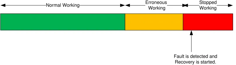
There is widespread use of reactive fault detection mechanisms for fault detections. These systems detect a fault after its occurrence and start the recovery henceforth. Such systems though provide good fault tolerant solution for general computing environment but cannot fulfill the time constrains set by real time computing systems. Real time computing systems like hospital- patient monitoring system, air traffic regulation system, etc. have critical running time constrains, which need to be fulfilled for successful operation.

Normal Working Erroneous

Working

Stopped Working

[image:8.612.117.520.307.418.2]

Fault is detected and Recovery is started.

Fig. 1- Timeline for a Reactive fault detection system

Figure 1 shows the time line for working of a reactive fault tolerant system. Reactive fault tolerant system keeps a continuous check on the performance of various devices in the system. They regularly poll the device for failure status. If a failure is detected during the run of the system, it informs the fault monitoring system and does the related recovery process.

(9)

1.2.2 Predictive fault detection

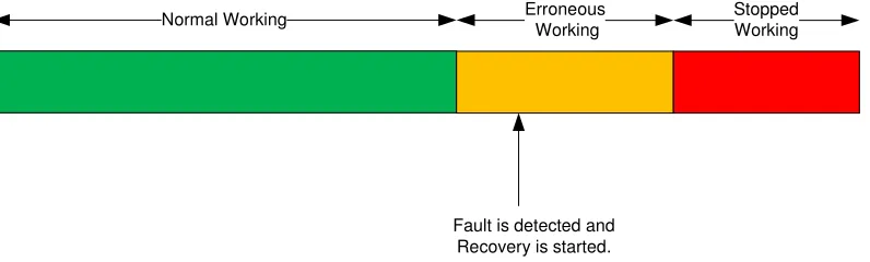
Predictive fault tolerant systems predict a fault before its occurrence, during the execution of the system, and hence are able to fulfill the time constrains set by real time systems.

Normal Working Erroneous

Working

Stopped Working

[image:9.612.113.511.169.289.2]

Fault is detected and Recovery is started.

Fig. 2- Timeline for a Proactive fault tolerant system

Predictive systems assume that faults, which are inherently unpredictable, do show some disruptive effect on the performance of the system [5]. Research studies show that faults do show a pattern of occurrence. Predictive fault tolerant systems exploit these patterns to predict a fault.

(10)

Failure rarity problem is a well-known issue for failure prediction algorithms. The annual hard disk failure rate is approximately 1%. Because of this, about thousand of disk drives need to be tested for more than an year to get data for about 15 failed drives [2]. This increases the false alarm rate, as less knowledge is available about the behavior of fault disks. This project tries to concentrate on reducing the false alarms with an optimum and elegant solution for fault prediction.

Project gives a detailed study and analytical comparison for two variations of SMART fault-prediction systems. SMART is used as a prediction algorithm in hard disks. The SMART algorithm predicts a fault in the system based on a set of predefined threshold values. It predicts a fault, if any of the threshold values are exceeded.

The Wilcoxon’s Rank Sum method, provided as a variation for SMART in [2], is basically tested for hard disk fault prediction. It predicts faults by comparing the behavior of the running device to a reference dataset. It assumes that faults do not have any pattern of occurrence and hence compares it with a reference set, generated from multiple device of the same type. This makes the prediction system very sensitive to erroneous predictions. Even a small temporal error value will generate a fault prediction. Hence this project presents combining DFT (Dispersion Frame Technique) with SMART, as a solution to reduce the false alarms. Rank-Sum is explained further in Section-2.

The DFT (Dispersion Frame Technique) developed at CMU for their MEAD architecture [7], predicts faults based on the error occurrence pattern in a given time frame. It tries to exploit the basic nature of ‘decreasing time frames’ for occurrence of errors. This project applies DFT on the warnings generated by SMART. i.e. Warnings generated by SMART are fed as input to the DFT algorithm, to find a pattern leading to failure predictions. DFT is explained in detail in section-3.

(11)

2 – Wilcoxon’s Rank-Sum Algorithm

The SMART (Self Monitoring and Reporting Technology) uses around some 30 different internal drive measurements. It uses pre-calculated thresholds for the individual attributes and checks the reading for each attribute against it. It then does a ‘OR’ operation on the result of each attribute. This can cause a high false alarm rate [2]. Hence the Wilcoxon’s Rank-Sum algorithm is proposed to replace threshold tests with rank comparisons for failure prediction. Rank Sum tests are recommended for rare failure events such as disk failures, rare disease, etc. where false alarm rates are high. They are particularly useful in cases where statistical distribution of the data is unknown and is suspected to be non-gaussian [2]. This algorithm is mainly tested for hard disk drive fault predictions.

The Rank-Sum algorithm, as the name indicates, sorts a group of reference data points and warning data points and ranks them according to the sorted position. Rank sum does not use the conventional threshold comparisons used for SMART. It calculates the standard deviation for the given set of warning data points. Any warning point found to deviate higher than an acceptable value is detected as a fault behavior. This is done for each attribute in question and their results are then ‘OR’ed. Fig. 4 shows the application of Rank-Sum on a set a data points.

[image:11.612.125.450.389.617.2]

Sorted data 5 5 5 5 5 6 6 9 Ranks 3 3 3 3 3 6 6 8 Reference ranks 3 6 3 3 3 Warning ranks 3 6 8 Reference data 5 6 5 5 5 Warning data 5 6 9

(12)

2.1 Rank-Sum Working

Following is given stepwise working for the Rank-Sum algorithm:

Step 1: The Warning dataset for each drive is taken to be its last five sample reads for each attribute. The Reference dataset for each attribute is taken to be 50 random samples averaged over multiple good drives. The will-fail drives are not included in the reference set values. The optimum dataset size will vary depending on time intervals of attributes being read and certain other factors [2].

Step 2: Sort these combined set of values and rank them accordingly. An average rank is given to the items that have the same value. i.e. If three values in the set are 0 and they have the rank{1,2,3}, all three of them will be given the rank ‘2’. Fig.4 shows a set of reference and warning data sorted and ranked for their values.

Step 3: Check if the ranks for warning data exceed the ranks for the reference data. In fig.4 the warning data value of ‘9’ with rank ‘8’ exceeds the rank limits of reference data [3-6], hence indicating a possible error. Warning data ranks exceeding the reference data ranks will indicate the warning data points to be very low or high in value.

Step 4: If the warning points exceed the reference point ranks, calculate the variance and hence standard deviation for the set of warning data points. For fig.4, variance for warning point ranks {3,6,8} is calculated from the mean rank ‘4.375’. Further, Standard deviation is calculated. If the standard deviation calculated exceeds a pre set limit for tolerable deviation, a warning is generated.

This is done for each attribute and all individual results are then ‘OR’ed to give a final result.

As observed from the working of the Rank-Sum algorithm, it does not assume a particular behavior pattern for the disk drive. It compares the incoming behavior of the disk drive to the pre-calculated behavior pattern stored for reference. This reference data is a collection of good working disks. It thus predicts a warning, if the incoming pattern differs comparably from the reference pattern. [2] gives a more detailed explanation for Rank-Sum.

(13)

3 - Dispersion Frame Technique

Dispersion Frame Technique is a prediction algorithm developed at CMU for their MEAD system. “DFT is implemented in a distributed online monitoring and predictive diagnostic system for their existing campus wide Andrew file system” [7]. Error logs for this predictive system were collected from 13 file servers over a period of 22 months [7]. [7] shows the descriptive study of the error log data analysis using joint probability statistics, statistical Weibull fit and DFT. The comparative results shown in [7] indicate DFT having highest success rate with least false alarms [7].

DFT uses intermittent and transient faults occurring during the run of the system to predict individual device failures. It determines the relationship between the error occurrences by examining the inter arrival time and the domain of their occurrence [7]. Knowledge gained in separating error logs into their constituent error sources and experiences of their hardware technicians were used for generating heuristics for DFT [7].

Time

i - 4 i - 3 i - 2 i - 1 i

Frame (i-3)

Frame (i-2)

Frame (i-1)

3,3 Warning

4 decreasing Warning 2,2 Warning

Index = 3

Index = 2 Index = 2

[image:13.612.105.520.321.484.2]

Index = 1 Index = 1

Fig.3 – Dispersion Frame Technique [7]

(14)

3.1 DFT Working

DFT predicts faults by finding relationships between occurrences of fault events in terms of their vicinity in time and the source of their occurrence. Based on the statistical analysis done [7], a dispersion frame of less than 168 hours was used to activate the DFT algorithm.

The DFT works as follows [7]:

Step 1: A time line of five most recent errors is taken into account for each device. DFT is activated when a frame size of less than 168 hours is encountered. Fig. 3 shows a decreasing time line for error occurrences.

Step 2: Each error occurrence on the time line is centered on by the previous two time frames. Fig. 3 shows frame for event (i-3), the inter arrival time between events (i-4) and (i-3), centered around error events (i-3) and (i-2). Similarly frame (i-2) is centered on (i-2) and (i-1).

Step 3: EDI is calculated as the number of errors from the center of each frame to its right most end. Fig. 3 shows the EDI of 3 for frame (i-3).

Step 4: A failure warning is issued under any of the following conditions:

(a)- 3.3 rule: If successive application of the same frame results in EDI of at least 3. In other words, it represents a scenario of steeply reducing dispersion frame (inter occurrence in time for error) as compared to a previous frame. In Fig. 3, 3.3 rule can be applied on frame (i-3). Frame (i-2) is very small as compared to frame (i-3).

(b)- 2.2 rule: If application of successive frames exhibits an EDI of at least 2. It differs from rule 3.3 as it considers uniformly decreasing time frames. Fig.3 shows that frames (i-3) and (i-2) show an EDI of at least 2 and hence 2.2 rule can be applied there.

(c)- 2 in 1 rule: A failure warning is generated if a dispersion frame is less than 1 hour in length.

(d)- 4 in 1 rule: If four errors occur within a 24 hour.

(15)

Step 5: Multiple iterations of step 2,3 and 4 are usually executed before issuing a failure warning.

As observed from the working of the algorithm, DFT considers the pattern of occurrence for errors during the working of the device. It assumes that more number of errors will occur with less inter arrival time during the life of a faulty device. A good working device on the other hand will not have such an error pattern. This assumption plays a major role in Dispersion Frame Technique for fault prediction. [7] describes in detail the working of DFT and the statistics about the heuristics used.

(16)

4 - Proposed Project

This project is to develop a simulation environment for simulating proactive prediction in a distributed system. This includes developing a language for simulation and writing a parser to generate the simulation environment, during the initial stage of the project. Two fault prediction algorithms – ‘the DFT algorithm’ and ‘Rank-Sum algorithm’ are implemented and integrated to work in the simulation environment. A real time dataset and synthetic dataset are used for testing and result collection purpose. The following sections describe in detail the architecture and high-level implementation of the project. Section 4.3 gives the definition and usage for the language used to define the distributed system in simulation. Section 4.4 and 4.5 gives the algorithm implementation details and dataset preparation details respectively. Section 4.6 shows the GUI snapshots for the simulation.

4.1 Architecture Diagram

Fig.5 illustrates the architecture diagram for this project. It gives an overview of the structure of the simulation system using a tree representation of the generated environment.

A text file containing the definition of the system in the language format described in section 4.3 is given as input to the simulation system. This input is fed to the parser. The parser parses the given environment definition and creates an equivalent environment in simulation. A GUI shown in section 4.6 is also generated for user viewing purpose.

(17)

W a rn in g P ro p a g a ti o n W a rn in g P ro p a g a ti o n W a rn in g P ro p a g a ti o n Simulation Input File Parser Definition for the

Simulation System

Simulation Environment Generates simulation setup

Network 1 Network 2

System 1

RAID 1

Disk 1 DISK 2 DISK 3

Behavior File Get current Reading

Behavior File Behavior File

[image:17.612.100.516.84.567.2]

Get current Reading Get current Reading Algorithm is Applied and Checked for Warning generation W a rn in g P ro p a g a ti o n

Fig.5- Architecture Diagram

(18)

4.2 Flow diagram

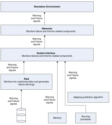
Below is shown a flow diagram, giving a detailed explanation of detection of a warning or error in the lower level devices and flow of that warning in the simulation system. Figure 6 shows process done at each level in the simulation environment.

Simulation Environment

Networks

Monitors failure and Informs related components

System Interface

Monitors failures and Informs related components

Raid

Monitors the underlying disks and generates failure warnings

Memory Running

processes

Applying prediction algorithm Warning

and Failure signals

Warning and Failure

signals

Warning and Failure

signals

Warning and Failure

signals

Warning and Failure

signals

Warning and Failure

[image:18.612.107.498.192.627.2]

signals

(19)

Fig.6 shows the higher-level implementation for this project. The simulation works in the following steps:

1- Each individual component, i.e. disk, memory and process, read their respective behavior from a predefined file.

2- A failure prediction algorithm is invoked if necessary pre-failure conditions appear. Each individual component checks for its failure status at a fixed interval. If a warning or error condition is met, each device will inform its parent/enclosing device/system. E.g. If a RAID exist in the system, the individual disk failures will be reported to the RAID controller. Similarly, if any of the RAID, disk, memory or process qualifies any warning condition, they will report this to the parent interface.

3- A Raid can be configured for failure based on the number of tolerable disk failures. Eg. A Raid of 5 disks can be configured to declare as failed, if 3 of the 5 disks fail. Failure of one disk will not result in a Raid failure.

(20)

4.3 Language for Simulation

This project consists of defining a simulation language, which allows creation of a distributed environment for simulation purpose. The below defined language allows you to define an environment consisting of single or multiple networks. Each network can then be defined to hold single or multiple machines. Every machine can have one or more memory, disk or raid array. Also every machine can have single or multiple processes running on them. A RAID can be configured for the minimum number of disk failures to call it a RAID failure. Each of the lower end components (disk, memory and process) can be configured to use a file to read its running behavior. This language also facilitates to define the dependencies between systems. Given below is the grammar for the proposed language.

Simulation ::= (Definition | RelationDef)+ <EOL>

Definition ::= DEFINE (EnvironmentDef | NetworkDef | SystemDef |

MemDef | DiskDef | ProcDef | RaidDef) END; <EOL>

EnvironmentDef ::= ENVIRONMENT Id: <EOL> NetDeclare+

NetworkDef ::= NETWORK Id : <EOL> (SysDeclare | NetDeclare)+

SystemDef ::= SYSTEM Id : <EOL> (ProcDeclare | DiskDeclare |

MemDeclare | RaidDeclare)+

MemDef ::= MEMId; <EOL> RUNNING FileName ; <EOL>

DiskDef ::= DISKId; <EOL> RUNNING FileName ; <EOL>

ProcDef ::= PROCId; <EOL> RUNNING FileName ; <EOL>

RaidDef ::= RAIDId; <EOL> DiskDeclare+

RelationDef ::= RELATION IdDEPENDS_ONId; <EOL>

NetDeclare ::= NETWORKId; <EOL>

SysDeclare ::= SYSTEMId; <EOL>

DiskDeclare ::= DISKId ; <EOL>

ProcDeclare ::= PROC Id; <EOL>

DiskDeclare ::= DISK Id; <EOL>

RaidDeclare ::= RAID Id Number ; <EOL>

Id ::= [a-zA-Z][ a-zA-Z_0-9]*

Number ::= [0-9]+

FileName ::= Id (.Id)?

<EOL> - defined as the newline (\n_{) character in a UNIX environment or}

(21)

Semantic Rules for the language:

1. Each Element needs to be declared before defining it. Here, each declaration is equivalent to creating an object and each definition is equivalent to configuring the component for its parameters

2. The Container needs to be declared and defined before the contained element. E.g. ‘Environment’ needs to be declared and defined before the ‘Networks’.

3. The first component to be declared has to be an ‘Environment’. Two environments can co-exist. But they cannot be related.

4. Each Component can declare multiple components in its definition. E.g. ‘Environment’ can contain multiple ‘Networks’ and a ‘Network’ can contain multiple ‘Systems’.

5. Each declared component need not be defined.

6. Declaration of a ‘Raid’ takes the number of disks whose failure can be tolerated by the system as ‘DiskDeclare’ parameter.

7. ‘Relation’ defines a dependency relationship between two components. Both the components involved in a ‘Relation’ need to be defined before defining a dependency between them.

8. Id can be any alphanumeric starting with an alphabet. 9. FileName can be any text file with a single ‘.’ extension.

Following is an example that will clarify the grammar usage:

DEFINE ENVIRONMENT env1 NETWORK N1;

END;

Here an environment ‘env1’ is defined. It contains a declaration for a Network ‘N1’. User can declare one or more networks in an environment.

DEFINE NETWORK N1: SYSTEM SYS1;

SYSTEM SYS2; END;

Similarly, the definition of each network can contain multiple systems.

DEFINE SYSTEM SYS1: PROC PROC1;

(22)

Defining a system involves declaring single or multiple components in it. Note that declaration of RAID array is followed by a number indicating the count of disk failures that can be tolerated during the normal run of the system.

DEFINE RAID RAID1: DISK DISK2;

DISK DISK3; DISK DISK4; END;

The definition of a raid array should contain disks more than the declared tolerable number of disks.

DEFINE DISK DISK2:

RUNNING simulation_testing_100002.csv; END;

Each end level component like Memory, Disk and Procedure can be defined to have a file giving their readings for their run. If an end component does not specify a running file, it will be assumed to be running good throughout the simulation lifetime.

RELATION SYS2 DEPENDS_ON SYS1;

Users are allowed to define a relationship between two systems or networks, in terms of their dependence. Here the above declaration allows SYS2 to be defined as a dependent on SYS1. This declaration needs both the systems to be created before defining their relationship. Any fault or failure in SYS1 will result in a respective fault or failure in SYS2.

NOTE:

[1] - This language needs the components to be defined in their order of sub-grouping. i.e. the enclosing components in the architecture should be declared before the enclosed one ( E.g. a machine should be declared and defined before the disk contained in it.)

[2]- This language expects unique names of the components. i.e. no two devices can have the same name. Unique names were not possible in coding as definitions are allowed anywhere irrespective of the parent component, leaving no option to identify similar named components uniquely.

(23)

4.4 Implementing DFT and Rank Sum algorithms

The description and working details for these algorithms are given in section 2 and 3. The DFT uses error thresholds from SMART to identify an incoming error and predicts a fault based on the pattern of these error occurrences. Rank-Sum on the other hand compares incoming values with reference values in order to generate a failure prediction. These algorithms are implemented in Java and integrated to a JavaSwing GUI for visualization of the fault prediction process. Screen shots for the GUI are given in section 4.6.

The project allows choosing one of the prediction techniques using a command line parameter at the start of the simulation run. Multiple instances of this simulation can be run for similar/different simulation environment definitions and algorithms in a JVM.

The data sets used for testing and result collection purpose are the real time working statistics for hard disk. More about the dataset is given in section 4.5.

4.5 Dataset preparation

The dataset used in this project is a real time statistical data for hard disks available at ‘http://cmrr.ucsd.edu/people/hughes/smart/dataset/’. Detailed description for this dataset is given in [3]. This dataset is in ‘.arff’ format and contains data of 64 attributes for 178 good working disks (disks that did not fail during their working lifetime) and 191 bad working disks (disks that ultimately failed during their lifetime of operation).

4.5.1 Dataset analysis

The dataset used here, is a raw dataset containing 64 attributes. Analysis was done on this dataset to remove the unwanted attributes and find valid thresholds for each attribute. WEKA and Microsoft access facilities were used for statistical analysis of the dataset. Data mining using WEKA and MS SQL server were done on this dataset to find some patterns for prediction purpose. Analysis using data mining reveal little about the dataset and hence statistical analysis was used for this purpose.

(24)

Both DFT and Rank-Sum, use this dataset in different ways according to their requirement for fault prediction purpose. The following sections give a detailed understanding of how this dataset is further refined and used by both algorithms.

4.5.2 Dataset modification for Rank-Sum

Rank-Sum algorithm uses reference dataset, made up of good working disk data, as a reference for comparing the considered disk behavior. It compares the incoming disk pattern with the reference pattern for every time interval. Rank-Sum algorithm does not assume a disk working to follow any particular pattern. Hence it compares the incoming behavior with a reference set made of good disk behaviors for a disk of same type. Figure 8 shows the usage of the dataset for the Rank-Sum algorithm.

Raw Dataset

Reference File Reference File

generation

Ranksum Algorithm File containing data for single

disk Single file extration

Input to Ranksum

Compare reference values

[image:24.612.161.528.295.483.2]

Fault Predictions O/P

Fig. 8 Use of dataset for Rank-Sum

(25)

4.5.3 Dataset modification for DFT

DFT algorithm uses threshold values for each attribute in the dataset to detect abnormal behavior in order to predict a possible failure. In order to simulate this behavior, the threshold values for all 24 attributes in the dataset were needed. [7] states that, threshold values for each disk attribute are normally given by the disk manufacturer. For this project, statistical analysis on the good and bad drives is used to get threshold values for each attribute. Figure 7 shows the use of datasets for DFT.

Raw Dataset

Threshold file Statistical

Analysis

DFT Algorithm File containing data for single

disk Single file extration

Input to DFT

Refer threshold values

[image:25.612.163.528.224.416.2]

Fault Predictions O/P

Fig. 7 Use of dataset for DFT

(26)

4.5.4 Synthetic dataset

A synthetic dataset is generated in the project for verifying the prediction accuracy for DFT algorithm, given optimum thresholds. The used raw dataset, do not provide enough information to verify the nature of the algorithms. This is because of the fact that reference set used for Rank-Sum is generated from the dataset itself, making Rank-Sum more accurate. Hence, a synthetic dataset is used to verify fault prediction accuracy for both algorithms.

(27)

4.6 Front-end GUI

[image:27.612.109.552.166.470.2]

This project has a GUI front-end developed in Java Swing for visualizing the fault prediction mechanism on a time line. It allows the user to visualize the behavior of the fault prediction algorithm on the simulated distributed system. Following are the snapshots for the simulation system.

Fig. 9 Snapshot for normal working of the simulation

Fig. 9 gives a snapshot for the normal working of the simulation. It shows various devices like disks, memory, process and raids depicted in different colors. All lower level configurable devices are colored GRAY. The GREEN colored rectangle shows the time line for each device. This rectangle grows with passing of time intervals. The GREEN color indicates normal working of the devices. The system, network and environment are shown as different colored panels.

(28)

[image:28.612.109.553.108.419.2]

Fig. 10 shows the snapshot for the simulation when the fault prediction algorithm predicts a warning.

Fig. 10 Snapshot for generation of a warning in Simulation

Fig. 10 shows the simulation system GUI state when a warning is generated. The rectangular time line shows the warning predictions for a time interval colored as ORANGE. Fig. 10 shows all related components colored ORANGE when a warning is generated. Here Disk3 has an abnormal behavior and hence warning is generated during its working. Disk3 is a part of Raid1 and hence Raid1 also shows a warning. Similarly SYS1, N1 and env1 are also colored ORANGE. Here, SYS2 is dependent on SYS1 and hence it also is colored ORANGE. Disk4, Disk5, Mem1 and Proc1 show a normal behavior.

(29)

Fig. 11 shows a snapshot for the simulation system when a component failure occurs.

Fig. 11 Snapshot for failure of a component in simulation

[image:29.612.103.561.107.421.2]

(30)

5 – Result Collection and Analysis

The main emphasis of this project is to understand the Output/Warning patterns for Rank-Sum and DFT for a given set of disk data. Experiments are conducted for collecting behavior statistics for both algorithms. The dataset to be used is given in [3]. The dataset contains real time statistics for the working of hard drive disks. The dataset has been studied and modified as needed, so as to meet the requirements of the project. The modifications for the dataset are explained in section 4.5. Other measures to be considered for comparing these algorithms are prediction accuracy and prediction precision.

5.1 Behavioral analysis for Rank-Sum

Rank-Sum algorithm, as mentioned in section 2, compares the incoming attribute values to a set of reference values for a given interval of time. If the incoming value exceeds the threshold of reference values, a warning is generated. Figure 12 is a snapshot for the working of the Rank-Sum algorithm.

Fig.12 Snapshot for Rank-Sum

(31)

5.2 Behavior analysis for DFT

This project uses DFT as an error pattern recognizer for the errors generated from SMART. In other words, the errors generated from applying SMART on the incoming values are fed to DFT for error pattern recognition. DFT predicts a warning, if any of the error conditions (section 3.1) are met. Figure 13 is a snapshot for the working of the DFT algorithm. This snapshot is for the same disk data used for Rank-Sum in fig.12.

Fig.13 Snapshot for DFT

Here fig.13 shows that DFT predicts the warning in the 136th hr. DFT tries to find a pattern for error occurrences and hence is less sensitive to sudden abnormal behaviors encountered during the run of the system.

5.3 Prediction Accuracy

Accuracy is a measure of how exact the prediction of the algorithm in question is. In other words, this is the measure of the false alarms generated by the system. Accuracy is an important metric to be considered, as false alarms can incur high cost to vendor/system owner. Accuracy is often considered as a starting point for analyzing the quality of a predictive model [6].

Both Rank-Sum and DFT were tested for a set of 30 good and 26 bad disk drives, for calculating the prediction accuracy. Using the formulas given in [6], prediction accuracy can be calculated as follows:

Rank-Sum Algorithm DFT Algorithm

[image:31.612.319.490.565.657.2]

Table 5.3.1 Table 5.3.2

Prediction Accuracy = 83.9% Prediction Accuracy = 75% Predicted

Negative

Predicted Positive Negative

Cases 26 4 Positive

Cases 5 21

Predicted Negative

Cases 30 0 Positive

(32)

Results show that Rank-Sum gives higher prediction accuracy as compared to DFT.

Detailed analysis reveal that DFT identifies all good drives as good but is not able to generate warnings for all bad disks. This is because of the fact that not all bad-working disks have enough data for error pattern generation. Also, the threshold values for SMART play an important role in error identification. An optimum threshold value can improve its prediction accuracy further.

Rank-Sum, as expected behaves very sensitive to the change in values of the incoming data. As shown in the table 5.3.1, Rank-Sum generates warning for 4 good working disks. On the other hand, it is able to identify more bad working disks as compared to DFT because of its ability to recognize sudden spurts of abnormal behavior.

5.4 Prediction Precision

Precision gives the measure of how precisely in time was the warning generated by the algorithms. This may allow us to distinguish the algorithms by when the warnings are generated in the time frame (early / late warnings). Certain applications may need an early warning whereas the others may need a just in time warning. This factor can help in choosing an algorithm based on the specified tradeoff.

This project involved testing both the algorithms for 26 bad working drives and collect prediction statistics in their time frames. Graph 5.4.1 gives a comparison for Rank-Sum and DFT for their warning predictions.

Precision Graph 0 50 100 150 200 250 300 350 400

0 5 10 15 20 25 30

(33)

In graph 5.4.1, the blue dots represent the prediction in time for DFT algorithm and the pink dots represent the prediction in time for the Rank-Sum algorithm. As observed in the graph, Rank-Sum algorithm generates warnings way ahead in time as compared to DFT. This gives a trade-off between the two algorithms. Rank-Sum can be used for sensitive applications where failure prediction well advance in time are useful and false alarms are not of much concern. Whereas, DFT can be used where false alarms can cost heavily and the system requires just in time failure predictions. Further research can be done on the threshold values used for DFT to improve its failure predictions.

5.5 Prediction Accuracy using Synthetic Dataset

Here, synthetic dataset is used to justify that improving the threshold values can result in improvement of prediction accuracy for DFT. The dataset used has rows with data values exceeding the pre-calculated threshold values. Results are collected for 20 bad working synthetic disks. Modifying table 5.3.1 and 5.3.2 to include results of synthetic data for bad working disks, we get

Rank-Sum Algorithm DFT Algorithm

Table 5.4.1 Table 5.4.2

Prediction Accuracy = 92% Prediction Accuracy = 96%

(Rank-Sum) (DFT)

Above calculations show that, if better defined threshold values are used, DFT can predict much accurately. Also an observation to be noted is that, the device needs to run long enough to at least generate 3 errors (2 dispersion frames), for DFT to identify the error.

As a conclusion of this section, we can conclude that Rank-Sum can predict majority of failures, but may be too early in time. As compared to this, DFT gives just in time prediction, but is restricted by the need to identify a pattern for errors, which may not exist always.

Predicted Negative

Cases 30 0 Positive

Cases 2 18 Predicted

Negative

Cases 26 4 Positive

(34)

6 - Limitations of Proactive prediction systems

A predictive fault tolerant system cannot replace a reactive system. This is due to that not every fault having a pattern of occurrence or show pre-occurrence symptoms, making them impossible to predict.

Also, failure is a rare event. Enough statistics are not available to know the behavior or pattern followed by bad working devices. i.e. More information about good working disk is available. This makes achieving good failure prediction accuracy difficult. In order to overcome this, we may try to keep wider fault prediction ranges, leading to higher false alarm rate and making failure prediction much complicated process.

Proactive predictive systems, though very useful, can cause considerable overhead on the performance of the system. They need the prediction mechanism to be activated every time the heuristics match, which may quite often reduce the system performance.

Because of all these reasons, proactive systems cannot, as yet, replace the reactive fault recovery systems.

7 - Future Enhancements

Future enhancements for this project includes, research on the different datasets for further analysis of the algorithms. As mentioned in section 5, there is a scope for improving these algorithms by improving the reference dataset and threshold values used by Rank-Sum and DFT respectively. Using more datasets and research on the behavior of the disks can help in modifying the algorithms as needed for better prediction accuracy.

Datasets for working of memory and process can also be gathered and used for the same or different algorithm in simulation. The simulation language supports creation and use of memory and processes for prediction monitoring purpose. Hence, this simulation of distributed environment can further be extended to include specific or generalized prediction algorithms for memory and processes.

(35)

Conclusion

This project was to develop a simulation for a distributed system and integrate fault prediction algorithms into it. It included developing a language for automatic generation of the simulation system, given a file containing its definition. It further included developing and integrating the prediction mechanism with the simulation environment. Project also included detailed study, analysis and modification of a real time dataset for hard disks so as to use it for result collection purpose.

(36)

Reference

[1]- F. Pfisterer and L. Lehmann, “Processor System Modeling- A language and simulation system”, Proceedings of the 4th symposium on Simulation of computer systems, 1976.

[2]- G. F. Hughes, J. F. Murray, K. Kreutz-Delgoda and C.Elkan, “Improved Disk Drive Failure Warnings”, IEEE Transaction on reliability, September 2002.

[3] - J. F. Murray, G. F. Hughes, K. Kreutz-Delgado, "Comparison of machine learning

methods for predicting failures in hard drives", Journal of Machine Learning Research, volume 6, 2005.

[4] – Selic Brian, IBM Developer, Fault Tolerant Techniques for Distributed Systems, http://www-128.ibm.com/developerworks/rational/library/114.html, July 2004.

[5] - T. A. Dumitras and P. Narsimhan, ”Fault-Tolerant Middleware and the Magical 1%”, ACM/IFIP/USENIX Conference on Middleware, Grenhole, France, November-December 2005.

[6]- Wikipedia, Accuracy Paradox, http://en.wikipedia.org/wiki/Accuracy_paradox, May 2007.

[7] -Y. Lin and D. P. Siewioek, “Error Log Analysis: Statistical Modeling and Heuristic Trend Analysis”, IEEE Transaction on Reliability, vol. 39, No. 4, 1990 October.