Spectral Reordering of a Range-Dependent
Weighted Random Graph
Desmond J. Higham
∗July 6, 2004
Abstract
Grindrod [Range-dependent random graphs and their application to modeling large small-world proteome datasets, Physical Review E, 66, 2002] posed the problem of reordering a range-dependent random graph and showed that it is relevant to the analysis of datasets from bioinformatics. Reordering under a random graph hypothesis can be regarded as an ex-tension of clustering and fits into the general area of datamining. Here, we consider a generalization of Grindrod’s model and show how an existing spectral reordering algorithm that has arisen in a number of areas may be interpreted from a maximum likelihood range-dependent random graph viewpoint. Looked at this way, the spectral algorithm, which uses eigen-vector information from the graph Laplacian, is found to be automatically tuned to an exponential edge density. The connection is precise for optimal reorderings, but is weaker when approximate reorderings are computed via relaxation. We illustrate the performance of the spectral algorithm in the weighted random graph context, and give experimental evidence that it can be successful for other edge densities. We conclude by applying the algorithm to a dataset from the biological literature that describes cortical connectivity in the cat brain.
keywords: bioinformatics, cortical connectivity, clustering, functional mag-netic resonance imaging of the brain, genome datasets, Laplacian, maximum likelihood, small world networks, sparse matrix, two-sum.
AMS: 65F50, 68R10
∗Department of Mathematics, University of Strathclyde, Glasgow G1 1XH, UK. Supported
1
Background
Grindrod [8, 9] recently defined a new class of range-dependent random graphs
that generalize the Watts/Strogatz small world framework [14, 19] and have great potential as models for interaction networks in bioinformatics. Take nodes la-belled v1, v2, . . . , vN and suppose that an edge connecting vi to vj exists with independent probability pij := g(|i−j|), for some suitable function g. Equiva-lently, the adjacency matrix A ∈ RN×N has aij = 1 with probability g(|i−j|) and aij = 0 otherwise. In this framework there is an underlying ordering of the nodes, and the edge probabilities are functions of the “lengths” of the edges. In typical small world networks, short range connections (|i−j| small) are much more frequent than long range connections (|i−j| large) and hence range depen-dent random graph models where g(k) decays rapidly as k → ∞ are of interest. Grindrod suggested edge probabilities of the formg(k) =αβk−1, forα, β ∈(0,1),
and showed how various characteristics, such as the expected vertex degree, are easily derived. He also gave experimental evidence that these networks capture the connectivity structure seen in proteome interaction data.
In addition to providing a model for interaction data, Grindrod’s work also suggested a fascinating inverse problem for extracting structural information. Given a network, that is, a set of nodes with all connections specified, how do we reorder the nodes so that any bias towards short range connections becomes apparent? In other words, how do we reorder a seemingly arbitrary network into one where the short-range/long-range connectivity patterns are revealed? Extracting this information is akin to, but more general than, clustering. In the bioinformatics context a suitable reordering reveals functional relationships and may drive further data collection. It gives answers to questions like:
• Which other genes/proteins behave like gene/protein X?
• What are the most likely false positives/false negatives in the data?
• Should a weakly observed interaction be classified as true or false?
A useful reordering algorithm must be robust with respect to erroneous data, including outliers—this rules out many methods from deterministic graph theory and sparse matrix computations.
In [10], we examined the potential of three sparse matrix reordering algorithms for unravelling random graphs. Here, we look at the most promising of these, spectral reordering, in the more flexible and general context of weighted edges.
of the problems is lost. Section 3 shows how the theory carries through to the case where edge weights are drawn from discrete distributions, and also to the case of directed graphs. In section 4 we use a simulation approach to test the results on a range of graphs, and in section 5 we apply the reordering algorithm to a dataset arising from a biological application.
2
Continuous Weights
In this work we extend Grindrod’s model to the case of an ordered graph with weighted edges. This allows for interaction data where, instead of “yes” or “no” quantification of similarity, there is a range of possible values, a generalization that is relevant to bioinformaticians, [1, 3, 5], and other bioscientists [11, 15]. For definiteness, we begin with undirected graphs and continuously weighted edges. We take the edge weights to be independent, non-negative, continuous random variables with range-dependent density. We remark that, in general, this leads to non-sparse networks. Our formal definition is as follows.
Definition 2.1 Given a set of edge density functions{f[k](x)}N−1
k=1, withf[k](x) =
0 for x <0, the corresponding continuously weighted undirected range-dependent random graph has nodes ordered 1,2,3, . . . , N with independent edge weights {wij}i<j, such that wij has density f[j−i](x).
Grindrod has advocated the name Renga1 for the range-dependent random
graphs analysed in [8, 9]. Thus, following a referee’s suggestion, we will use
the phrase C-Renga in place of the more cumbersome “continuously weighted
undirected range-dependent random graph” in Definition 2.1.
2.1
Reordering
We may now consider the reordering problem for a C-Renga. If, as would be typical in a bioinformatics application, the underlying range-dependent structure was believed to be present, but the nodes were ordered arbitrarily, can we find a reordering that reveals the structure? One way to formalize this question is to define an objective function that, given a particular ordering, measures how close the data is to C-Renga form. In Definition 2.2 we generalize the maximum likelihood approach of [8]; hereP denotes the set of all permutation vectors, that is, all orderings of the integers 1,2, . . . , N.
1A renga is a collection of haiku-like verses written by a network of poets. The word is both
Definition 2.2 Given an instance of a C-Renga with edge densities{f[k](x)}N−1
k=1,
but with the nodes in arbitrary order, a maximum likelihood reordering p ∈ P
solves
max p∈P
Y
i<j
f[|pi−pj|](w
ij). (1)
We note that the quantity to be maximized in (1) represents, for a given ordering p∈ P, the probability of that C-Renga arising.
Alternatively, given the general aim of having short-range edges with larger weights than long-range edges, we could reorder with respect to a two-sum objec-tive function. This idea, which dates back to [4, 16], has been used as the basis for minimizing fill-in during sparse matrix computations.
Definition 2.3 Given any undirected weighted graph with weights {wij}i<j, a
minimum two-sum reordering p∈ P solves
min p∈P
X
i<j
(pi−pj)2wij. (2)
Both maximum likelihood and two-sum reordering are hard, discrete opti-mization problems. However, as we mention in section 2.2, the two-sum version has a natural relaxation into a tractable eigenvalue computation. Definition 2.2 requires the C-Renga model, that is, the edge density functions{f[k](x)}N−1
k=1 , to
be specified. The two-sum reordering in Definition 2.3, by contrast, makes no reference to a model. However, as Theorem 2.1 shows, it is possible to identify the two-sum problem as a special case of maximum likelihood.
Theorem 2.1 A permutation p ∈ P solves the minimum two-sum reordering problem in Definition 2.3 if and only if it solves the maximum likelihood reordering problem in Definition 2.2 for the C-Renga model where f[k](x) is the density
function for the exponential distribution with parameter k2; that is, f[k](x) =
k2e−k2x
.
Proof. Set f[k](x) = k2e−k2x
in (1). Taking logs and negating converts the problem to
min p∈P
" X
i<j
(pi−pj)2wij −2
X
i<j
log|pi−pj|
#
. (3)
Since the second summation inside the min is the same for allp∈ P, the problem is equivalent to finding a minimum two-sum reordering.
2.2
Relaxed Reordering
For a large system, it is not feasible to examine all permutations p ∈ P in an attempt to optimize in (1) or (2). Grindrod [8] outlined a heuristic iterative algorithm that works directly with permutation vectors. Although the details of the algorithm were not given, impressive results were obtained on synthetic and real-life data.
Generalizing the approach in [10] we may investigate an alternative algorithm based on relaxing the problem to the continuous realm, where Lagrange multi-pliers can be exploited. This relaxation idea has proved successful for a number of applications in clustering, partitioning and datamining, [2, 4, 7, 17]. In order to define the relaxation process, we must also assume that the edge density ex-pressions {f[k](x)}N−1
k=1 continue to make sense when k is a positive real number.
(We note that this is the case for the exponential distribution in Theorem 2.1.) In the following, e denotes the vector in RN with all entries equal to one, and k · k2 denotes the Euclidean norm.
Definition 2.4 Given an instance of a C-Renga with edge densities{f[k](x)}N−1
k=1,
but with the nodes in arbitrary order, a relaxed maximum likelihood reordering
y∈RN solves
max y∈RN,kyk
2=1, yTe=0 Y
i<j
f[|yi−yj|](w
ij). (4)
Definition 2.5 Given any undirected weighted graph with weights {wij}i<j, a
relaxed minimum two-sum reordering y∈RN solves
min y∈RN,kyk
2=1, yTe=0 X
i<j
(yi−yj)2wij. (5)
Comparing Definitions 2.2 and 2.3 with Definitions 2.4 and 2.5, we see that
relaxation involves weakening p ∈ P to y ∈ RN and imposing the constraints
kyk2 = 1 and yTe= 0. We may recover a permutation p∈ P from a
componen-twise ordering ofy:
pi ≤pj ⇔yi ≤yj. (6)
The fact that such a p is invariant to scaling or shifting of y motivates the
normalization kyk2 = 1 and the orthogonality condition yTe= 0.
The relaxed two-sum problem has the advantage of being computationally tractable. It is easily shown that the objective function Pi<j(yi−yj)2wij may be written yT(D
−W)y, where W ∈ RN×N has (W)ij = (W)ji =wij and D = diag(Piwij). The matrixD−W is known as the Laplacian of the graph (although this term is also used for a different, but related, matrix, [6]). By construction,
D−W is positive semi-definite and has a zero eigenvalue corresponding to the
eigenvector e. It follows from the Courant-Fischer Minimax Theorem, see for
example, [12], thatyT(D−W)y, subject tokyk
finding the next smallest eigenvalue ofD−W and lettingybe the corresponding
normalized eigenvector. Computing a relaxed solution y and projecting back to
a permutation p satisfying (6), the key idea of [4], is what we mean by spectral reordering. The vector y is often referred to as the Fiedler vector of W, and we note that special purpose software is available for its computation, [13].
Theorem 2.1 shows that the discrete formulations of maximum likelihood re-ordering (1) and minimum two-sum rere-ordering (2) are equivalent, underf[k](x) =
k2e−k2x
. We now give two simple examples to show that this equivalence is lost under relaxation. The effect arises because the second summation inside the min in (3) becomes significant.
Example 1 Consider the case
W =
0 11 0 1α
α 1 0
, (7)
whereα >0 is a parameter. The eigenvalue/eigenvector pairs of D−W may be written {λi, vi}, where
λ1 = 0, λ2 = 1 + 2α, λ3 = 3
and
v1 =
1 √ 3 1 1 1
, v2 =
1 √ 2 − 1 0 1
, v3 =
1 √ 6 1 −2 1 .
It follows that for 0 < α < 1, λ2 is the second smallest eigenvalue, and the
relaxed minimum two-sum reordering is found by taking y = v2. Applying (6),
this projects to the permutation [1,2,3]T. It is clear that this is a true minimum two-sum reordering (2). Forα >1,λ3is the second smallest eigenvalue ofD−W,
so y = v3 gives the relaxed minimum two-sum reordering. Whichever way ties
are broken in taking the projection (6), this corresponds to movingαin (7) away from the corner, which solves the discrete problem (2). However, becausey =v3
does not have distinct components, it cannot possibly be a relaxed maximum likelihood reordering, (4), under the exponential distribution in Theorem 2.1.
Example 2 To examine a less pathological case in practice, we perturb Ex-ample 1 to
W =
0 1.1 2
1.1 0 1
2 1 0
. (8)
problems (1) and (2).) To compute a relaxed maximum likelihood reordering, we minimized the negative log likelihood
X
i<j
(yi−yj)2wij−2
X
i<j
log|yi−yj| (9)
overy∈R3 of the formy= cosθ v2+sinθ v3, wherev2 andv3 are the eigenvectors
corresponding to the middle and largest eigenvalues of D−W. Note that the
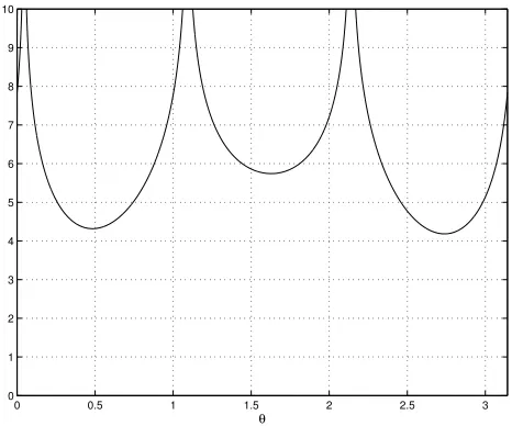
relaxed minimum two-sum reordering occurs atθ = 0. In Figure 1 we show how
(9) varies for θ ∈ [0, π]. The three local minima were found using MATLAB’s
fminbndand the overall solutionθ = 2.74 produced a relaxed maximum likelihood reordering that projects to [3,1,2]T (which does not solve the discrete problems (1) and (2)). This example illustrates that both the relaxed and the projected solutions may differ between two-sum and maximum likelihood formulations.
0 0.5 1 1.5 2 2.5 3 0
1 2 3 4 5 6 7 8 9 10
[image:7.612.175.408.257.451.2]θ
Figure 1: Negative log likelihood (9) for the example (8) using y = cosθ v2 +
sinθ v3.
We also remark that the behaviour of relaxed minimum two-sum reordering in those examples is consistent with [2, Theorem 3.3], which shows that if it is possible to reorder so that entries along any row are non-increasing as we move away from the diagonal, then the Fiedler vector will find this reordering.
Examples 1 and 2 show that we cannot prove a direct analog of Theorem 2.1 for the relaxed problems. However, a weaker version does hold.
Theorem 2.2 A vectory∈RN solves the relaxed minimum two-sum reordering problem in Definition 2.5 if and only if it solves the relaxed maximum likelihood reordering problem in Definition 2.4 for a C-Renga model where
f[k](x) =Ce−k2x
for any constant C (independent of k).
Proof. The result can be proved in a similar manner to Theorem 2.1.
We note that, given the data{wij}, a suitable density function for Theorem 2.2 can be constructed as
f[k](x) =
e−k2x
, 0≤x≤maxi<jwij,
ǫ, maxi<jwij < x≤Dk, 0, Dk < x,
whereǫ and Dk are chosen to make
R∞
0 f[
k](x)dx= 1.
3
Discrete Weights and Directed Edges
An alternative to the C-Renga setting is to allow the range-dependent edge weights to be drawn from a discrete distribution. Below, we spell out how the material in section 2 converts to this case.
Definition 3.1 Given a set of non-negative possible edge weights,{mr}Lr=1, and,
for each range 1 ≤ k ≤ N −1, a set of probabilities {fr[k]}Lr=1 with f [k]
r ≥ 0 and
PL
r=1f [k]
r = 1, the corresponding discretely weighted undirected range-dependent random graph has nodes ordered 1,2,3, . . . , N with independent edge weights {wij}i<j, such that P(wij =mr) = f[
j−i]
r .
Following the remark after Definition 2.1, we will use the phrase D-Renga
as an abbreviation for “discretely weighted undirected range-dependent random graphs” in Definition 3.1.
Definition 3.2 Given an instance of a D-Renga where the possible edge weights {mr}Lr=1 have probabilities {f
[k]
r }Lr=1, but with the nodes in arbitrary order, and writing wij =msij for i < j, a maximum likelihood reordering p∈ P solves
max p∈P
Y
i<j
f[|pi−pj|]
sij .
Theorem 3.1 A permutation p ∈ P solves the minimum two-sum reordering problem in Definition 2.3 if and only if it solves the maximum likelihood reordering problem in Definition 3.2 for the D-Renga model where the edge weights wij are members of the set{mr}Lr=1 with probabilities
fr[k]=
e−k2m
r
PL
j=1e−k 2mj.
Definition 3.3 Given an instance of a D-Renga with possible edge weights{mr}Lr=1
and edge probabilities{fr[k]}Lr=1, but with the nodes in arbitrary order, and letting
wij =skij for i < j, a relaxed maximum likelihood reordering y∈R
N solves
max y∈RN,kyk
2=1, yTe=0 Y
i<j
f[|yi−yj|]
sij .
Theorem 3.2 A vectory∈RN solves the relaxed minimum two-sum reordering problem in Definition 2.5 if and only if it solves the relaxed maximum likelihood reordering problem in Definition 3.3 for a D-Renga model where the edge weights
wij are members of the set {mr}Lr=1 with probabilities
fr[k]=Ce− k2m
r,
where C is a constant (independent of k).
Proof. The result can be proved in a similar manner to Theorem 2.2.
Given data wij from a set of edge values {mr}Lr=1, a suitable model for
The-orem 3.2 can be constructed by setting fr[k] = Ce−k
2m
r for 1 ≤ r ≤ L, where
the constant C is chosen so that PLr=1fr[1] <1, and then adding a dummy edge weight mL+1 and setting fL[k+1] = 1−
PL
j=1f [k]
j .
We also mention that this work extends readily to the case of directed graphs; that is, to unsymmetric W. The weights wij may be taken as i.i.d. with density
f[|j−i|](x) in Definition 2.1 and P(w
ij =mr) =f
[|j−i|]
r in Definition 3.1. The
cor-responding maximum likelihood reordering and minimum two-sum reordering are given by (1) and (2), respectively, withi < j replaced by i6=j. All previous the-orems remain valid. The relaxed problems are modified similarly, and a spectral reordering algorithm based on relaxation then uses the Laplacian of 12(W+WT) instead of the Laplacian ofW.
An unsymmetric W with discretely weighted entries is treated in section 5.
4
Computations on Weighted Random Graphs
When computing with the algorithm and visualizing the results, it is natural to work with inverses of reordering permutations. Letting p−1 ∈ P denote the
inverse of p∈ P, so that p−1
pk =k and pp−k1 =k, we note the identity
X
i,j
(pi−pj)2wij =
X
i,j
(i−j)2w
p−1
i p−j1, for any p∈ P.
It follows that a reorderingpin the sense of (2) may be regarded as replacing the matrix W by a new matrix whosei, jth entry is wp−1
i ,p−
1
j . We also note that the
MATLAB functionsortdirectly computes the inverse, p−1, of apsatisfying (6). For convenience, we use hats to denote permutations that represent inverses of reorderings, so pbcorresponds to p−1.
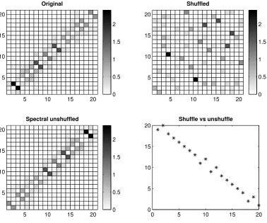
In Figure 2 we illustrate the spectral reordering algorithm on a C-Renga. We setN = 20 and generated weights aij fori < j as samples from a pseudo-random number generator using an exponential distribution with parameter (i−j)2. From
Theorem 2.1, this is the natural range-dependency for the two-sum objective function. The upper left-hand picture shows the 20×20 symmetric weight matrix,
M, using a grey-scale. The upper right-hand picture shows a shuffled version of this matrix. Here, a symmetric row and column permutation was applied—in other words, the nodes in the graph were swapped—using a permutation vector
b
q ∈ P. The resulting W, where wij = aqbi,qbj, is the data matrix to which the
algorithm was applied2. We computed the eigenvector y corresponding to the
second smallest eigenvalue of the Laplacian, and used this to induce the inverse
b
p of a permutation p ∈ P satisfying (6). Applying this permutation to the
shuffled matrix produced the matrix with entries wpbi,bpj shown in the lower
left-hand picture. Comparing the two left-left-hand pictures, we see that the algorithm has successfully moved the large weights towards the diagonal (that is, associated them with short-range edges), although it has not recovered the original matrix precisely. In the lower right-hand picture we compare the arbitrary shuffling that we used to generate the data matrix with the unshuffling computed by the algorithm. To do this we plot the vector{qbpbk}
N
k=1. If the unshuffling were exact
this would give points on a straight line of slope±1. We see that the algorithm has done a reasonable job of reverse engineering the shuffle. Nodes that were neighbors in the original C-Renga are no more than two places apart in the
computed solution. It is interesting to note that while p does a good job of
unshuffling q, the converse is not true. We have
{qbbpk} =
19 20 18 17 16 15 14 13 11 12 9 10 8 7 6 5 4 2 3 1 ,
{bpqbk} =
17 12 6 7 11 3 10 15 19 13 4 2 5 16 8 14 1 20 9 18 .
2Because node reordering represents a similarity transformation of the graph Laplacian,
In our context it is the ordering of bqbpk that matters—the task is to undo the
original shuffle.
5 10 15 20
5 10 15 20 Original 0 0.5 1 1.5 2
5 10 15 20
5 10 15 20 Shuffled 0 0.5 1 1.5 2
5 10 15 20
5 10 15 20 Spectral unshuffled 0 0.5 1 1.5 2
0 5 10 15 20
0 5 10 15 20
[image:11.612.103.481.105.420.2]Shuffle vs unshuffle
Figure 2: Upper left: C-Renga with exponentially distributed weights. Upper right: shuffled C-Renga. Lower left: unshuffled C-Renga from spectral algorithm, Lower right: comparison of shuffling and unshuffling.
Because the grey-scale pixel pictures become harder to interpret for biggerN, and because we want to report on a large batch of tests, we introduce two error measures. The first is
perr := min
max
1≤k≤N(|bqpbk−k|),1≤maxk≤N(|qbpbk −(N −k+ 1)|)
.
This is an indication of the accuracy of the unshuffle. The second is
twosumerr :=
P
i<j(i−j)
2
b
wij −
P
i<j(i−j)
2w
ij
P
i<j(i−j)2wij
,
where Wcij = wbpi,bpj is the computed unshuffled matrix, illustrated by the lower
reducing the two-sum, relative to the two-sum of the original C-Renga. (Note that the two-sum also has a log-likelihood interpretation, as shown by Theorem 2.1.)
In the example of Figure 2 we had perr = 1 and twosumerr =−0.0177. The
negative value for twosumerr indicates that the re-shuffled matrix has a smaller two-sum than the original.
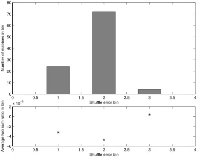
Figure 3 illustrates the performance of the algorithm on 100 instances of a C-Renga of dimensionN = 1000. As for Figure 2 we generated the weight matrices using an exponential distribution forwij with parameter (i−j)2. The histogram in the upper picture shows how many of the 100 matrices were unshuffled with perr = 0,1,2,3, . . .. In the lower picture, for the same binning of matrices, we give the average over that bin of twosumerr. We see that all cases have a shuffle error of 1, 2 or 3. Experiments with other dimensions suggest that the performance generally improves asN is increased.
0 0.5 1 1.5 2 2.5 3 3.5 4
0 10 20 30 40 50 60 70 80
Shuffle error bin
Number of matrices in bin
0 0.5 1 1.5 2 2.5 3 3.5 4
−6 −4 −2 0 2x 10
−5
Average two sum ratio in bin
[image:12.612.99.486.261.571.2]Shuffle error bin
Figure 3: Performance of spectral algorithm on 100 instances of a dimensionN = 1000 C-Renga with exponentially distributed weights. Upper plot: histogram of perr. Lower plot: average of twosumerr within each nonempty bin.
distribution over (0,1/(j −i)). These edge densities no longer match the
ex-ponential densities in Theorem 2.1, and the mean edge weight at a distance k
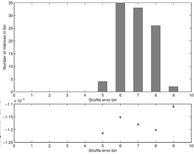
decays as O(1/k) rather than O(1/k2). Figure 4 shows the perr and twosumerr
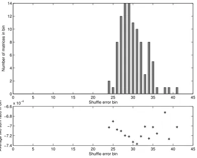
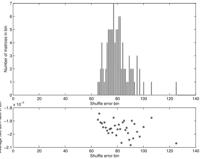
values that arose. We see that the algorithm has continued to perform well. Figures 5 and 6 give the corresponding results for weights uniformly distributed over (0,1/(j−i)α), with α= 0.5 and α= 0.25, respectively. With α reduced to 0.5 the algorithm still does a reasonable job of recovering ordering information.
As α is decreased the performance must, of course, degrade, and we see that
with α = 0.25 the reordered matrices differ significantly from the original data, although, on average, the two-sum is still well controlled.
0 1 2 3 4 5 6 7 8 9 10
0 5 10 15 20 25 30 35
Shuffle error bin
Number of matrices in bin
0 1 2 3 4 5 6 7 8 9 10
−1.25 −1.2 −1.15
−1.1x 10
−4
Average two sum ratio in bin
[image:13.612.100.491.219.530.2]Shuffle error bin
Figure 4: Similar to the computation in Figure 3, but with mij for i < j drawn from a uniform (0,1/(j−i)α) distribution, with α = 1. DimensionN = 1000.
5
Cat Brain Data
0 5 10 15 20 25 30 35 40 45 0
2 4 6 8 10 12 14
Shuffle error bin
Number of matrices in bin
0 5 10 15 20 25 30 35 40 45
−7.4 −7.2 −7 −6.8 −6.6x 10
−4
Average two sum ratio in bin
[image:14.612.100.491.60.373.2]Shuffle error bin
Figure 5: Similar to the computation in Figure 4, but with α= 0.5.
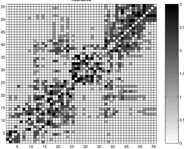
2 or 3 and the matrix is unsymmetric. Here, a portion of the brain has been divided into regions, and the value of entry (i, j) indicates the strength of the connectivity between regions i and j. A key issue here is to pull together well-connected regions (which need not be geographically close); that is, to reorder the matrix so that large entries appear near the diagonal. This allows biologists to identify parts of the brain that are likely to be involved in related activities. The required information may be a clustering of the data [11] or, more generally, a reordering [15]. The authors in [11] defined a suitable objective function and used an evolutionary algorithm to search over the set of permutation vectors, an approach akin to that of Grindrod [8], and reveal clusters. Figure 7 shows their solution. Computation time for the algorithm on a DEC ALPHA 3000-600 UNIX workstation was reported to range “from several hours to a few days”.
0 20 40 60 80 100 120 140 0
1 2 3 4 5 6 7
Shuffle error bin
Number of matrices in bin
0 20 40 60 80 100 120 140
−2.1 −2 −1.9 −1.8x 10
−3
Average two sum ratio in bin
[image:15.612.99.490.60.371.2]Shuffle error bin
Figure 6: Similar to the computation in Figure 4, but with α= 0.25.
3.4th power. Of course, the resulting reordering was applied to the original data. The question of whether there is an optimal way to preprocess a matrix before applying the spectral algorithm is an interesting area for future research.
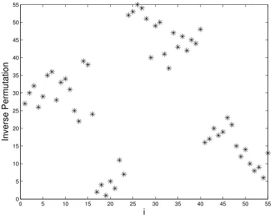
Figure 9 compares the two solutions by plotting the inverse of the permutation that maps Figure 7 into Figure 8. We see that the broad features of the two solutions are similar—both suggest four highly inter-connected blocks consisting of similar components, although the precise orderings are quite distinct. The two-sums for the matrices in Figures 7 and 8 are 3.5×10⁵ and 2.0×10⁵, respectively.
Of course, aside from using quantitative objective functions, such as the two-sum, the issue of “how good is a solution” would best be judged in terms of whether it extracts meaningful information for a biological scientist.
connectivity networks relating to the visual system.
5 10 15 20 25 30 35 40 45 50 55
5 10 15 20 25 30 35 40 45 50 55
Original
[image:16.612.131.508.99.403.2]0 0.5 1 1.5 2 2.5 3
Figure 7: Original, ordered cat brain data from [11].
6
Summary and Conclusions
The two main thrusts of this work were
• to extend Grindrod’s range-dependent random graph model to the
practi-cally relevant cases of weighted and undirected edges, and
• to show via analysis and numerical experiment that a spectral algorithm
gives an effective means to tackle the corresponding reordering problem.
5 10 15 20 25 30 35 40 45 50 55 5
10 15 20 25 30 35 40 45 50 55
Reordered
[image:17.612.132.506.71.373.2]0 0.5 1 1.5 2 2.5 3
Figure 8: Spectrally reordered cat brain data.
Acknowledgements Much of this work was done while I visited the Centre for Advanced Study, Oslo, during the Special Year in Geometric Integration. I am grateful to Heidi Johansen-Berg and Tim Behrens of the Oxford Centre for Functional Magnetic Resonance Imaging of the Brain for pointing me towards the dataset used in section 5.
References
[1] R. B. Altman and S. Raychaudhuri, Whole-genome expression analy-sis: challenges beyond clustering, Current Opinion in Structural Biology, 11 (2001), pp. 340–347.
0 5 10 15 20 25 30 35 40 45 50 55 0
5 10 15 20 25 30 35 40 45 50 55
i
[image:18.612.94.485.63.376.2]Inverse Permutation
Figure 9: Inverse permutation from spectral reordering of cat brain data.
[3] A.-L. Barab´asi and Z. Oltvai,Network biology: Understanding the cell’s functional organization, Nature Reviews Genetics, 5 (2004), pp. 101–114.
[4] S. T. Barnard, A. Pothen, and H. D. Simon, A spectral algorithm for envelope reduction of sparse matrices, Numerical Linear Algebra with Applications, 2 (1995), pp. 317–334.
[5] J. S. Chuang and D. Roth, Gene recognition based on DAG shortest paths, Bioinformatics, 1 (2001), pp. 1–9.
[6] F. Chung, Spectral Graph Theory, American Mathematical Society, Provi-dence, RI, 1997.
[8] P. Grindrod, Range-dependent random graphs and their application to modeling large small-world proteome datasets, Physical Review E, 66 (2002), pp. 066702–1 to 7.
[9] , Modeling proteome networks with range-dependent graphs, American Journal of PharmacoGenomics, 3 (2003), pp. 1–4.
[10] D. J. Higham, Unravelling small world networks, J. Comp. Appl. Maths, 158 (2003), pp. 61–74.
[11] C. C. Hilgetag, G. A. Burns, M. A. O’Neill, J. W. Scannell, and M. P. Young,Anatomical connectivity defines the organization of clusters of cortical areas in the macaque monkey and the cat, Phil. Trans. R. Soc. Lond. B, Biol. Sci., 355 (2000), pp. 91–110.
[12] R. A. Horn and C. R. Johnson,Matrix Analysis, Cambridge University Press, Cambridge, 1985.
[13] Y. Hu and J. A. Scott, HSL_MC73: A fast multilevel Fiedler and pro-file reduction code, RAL-TR-2003-36, Numerical Analysis Group, Computa-tional Science and Engineering Department, Rutherford Appleton Labora-tory, 2003.
[14] H. Jeong, B. Tombor, R. Albert, Z. Oltval, and A.-L. Barab´asi, The large scale organisation of metabolic networks, Nature, 407 (2000), pp. 651–654.
[15] H. Johansen-Berg, T. E. J. Behrens, I. Drobnjak, S. M. Smith,
D. J. Higham, and P. M. Matthews,Connectivity based anatomical par-cellation of cortical grey matter, 10th International Conference for Functional Mapping of the Human Brain, June 2004, Budapest, Hungary. Available on CD-Rom in NeuroImage, (2004).
[16] M. Juvan and B. Mohar, Optimal linear labelings and eigenvalues of graphs, Disc. Appl. Math., 36 (1992), pp. 153–168.
[17] J. Shi and J. Malik, Normalized cuts and image segmentation, IEEE Transactions on Pattern Analysis and Machine Intelligence, 22 (2000), pp. 888–905.
[18] S. H. Strogatz,Exploring complex networks, Nature, 410 (2001), pp. 268– 276.
![Figure 7: Original, ordered cat brain data from [11].](https://thumb-us.123doks.com/thumbv2/123dok_us/1722449.125645/16.612.131.508.99.403/figure-original-ordered-brain-data-from.webp)