Validating High Level Simulation Results against Experimental Data and Low Level Simulation : A Case Study

(1)

Data and Low Level Simulation : A Case Study

.

White Rose Research Online URL for this paper:

http://eprints.whiterose.ac.uk/151879/

Version: Accepted Version

Conference or Workshop Item:

Griffin, David Jack orcid.org/0000-0002-4077-0005, Harbin, James Robert

orcid.org/0000-0002-6479-8600, Burns, Alan orcid.org/0000-0001-5621-8816 et al. (3

more authors) (2019) Validating High Level Simulation Results against Experimental Data

and Low Level Simulation : A Case Study. In: Real-Time Networks and Systems, 06-08

Nov 2019.

[email protected]

https://eprints.whiterose.ac.uk/

Reuse

Items deposited in White Rose Research Online are protected by copyright, with all rights reserved unless

indicated otherwise. They may be downloaded and/or printed for private study, or other acts as permitted by

national copyright laws. The publisher or other rights holders may allow further reproduction and re-use of

the full text version. This is indicated by the licence information on the White Rose Research Online record

for the item.

Takedown

If you consider content in White Rose Research Online to be in breach of UK law, please notify us by

(2)

Data and Low Level Simulation: A Case Study

David Griin

University of York York, United Kingdom [email protected]

James Harbin

Alan Burns

Iain Bate

University of York York, United Kingdom

[email protected]

Robert I. Davis

University of York York, United Kingdom

[email protected]

Leandro Soares Indrusiak

ABSTRACT

Simulation can be considered a necessary evil in the validation of systems, especially when the system under consideration is being prototyped and therefore does not presently exist. This is com-pounded by the use of high level simulators; on the one hand, high level simulation is eicient, in that it abstracts away many details of the system which are deemed to be not important. This allows for a simpler and faster running simulator, which allows the user to obtain results faster and/or perform more experiments. On the other hand, some of the details abstracted away might turn out to be important, introducing inaccuracies.

This paper outlines a framework for the statistical understanding and attribution of the errors produced by a high level simulator when compared against real experiments by means of a low level simulator. This allows the user of a simulator to determine whether or not the inaccuracies are signiicant, and whether or not the high level simulator requires reinements in its accuracy for the results to be valid. These techniques are illustrated via a case study.

ACM Reference Format:

David Griin, James Harbin, Alan Burns, Iain Bate, Robert I. Davis, and Le-andro Soares Indrusiak. 2019. Validating High Level Simulation Results

against Experimental Data and Low Level Simulation: A Case Study. In27th

International Conference on Real-Time Networks and Systems (RTNS 2019), November 6ś8, 2019, Toulouse, France.ACM, New York, NY, USA, 11 pages. https://doi.org/10.1145/3356401.3356414

1 BACKGROUND

Components of a Cyber-Physical System (CPS) typically combine embedded processing, sensors, actuators and communication [2]. This allows the components of the CPS to locally process collected data before determining what should be communicated to other components of the system, for the purposes of either controlling the system or storing data. However, communication between diferent

Permission to make digital or hard copies of all or part of this work for personal or classroom use is granted without fee provided that copies are not made or distributed for proit or commercial advantage and that copies bear this notice and the full citation on the irst page. Copyrights for components of this work owned by others than the author(s) must be honored. Abstracting with credit is permitted. To copy otherwise, or republish, to post on servers or to redistribute to lists, requires prior speciic permission and/or a fee. Request permissions from [email protected].

RTNS 2019, November 6ś8, 2019, Toulouse, France

https://doi.org/10.1145/3356401.3356414

components presents a challenge: physical connections provide high bandwidth and low latency, but can be expensive to install. In some cases, such as on-body monitoring systems [10], a physical connection may not be possible. For these reasons, CPS may choose to use wireless communications.

Ωireless communications typically simplify the physical instal-lation of a CPS, but carry some signiicant trade ofs. Ωireless communications are not as reliable as a physical connection, for example being subject to background radiation [7], which can cause a given communication to fail. In addition, wireless systems have higher latency and lower bandwidth than physical connections [1, 14]. However, the beneits of wireless communications, in the form of lower installation and maintenance costs, in addition to en-abling systems which are inappropriate for wired communications, make wireless communications an attractive feature for CPS.

A recent topic of interest in the real-time community is that of Mixed Critically Systems (MCS) [18]. Mixed Criticality Systems pro-vide a mechanism by which in the unlikely event a high-criticality task is unable to complete given the resources it is given, resources can be diverted from lower-criticality tasks. This allows the system to continue to operate, albeit with reduced functionality. The tech-nique can also be applied to wireless communications, allowing high-criticality communications to have a high conidence of being delivered regardless of interference or limited resources.

In any scientiic discipline, the benchmark for accuracy is to take observations from the system under study - a ªreal experimentº. However, real experiments can be diicult to conduct. Probe efects [6] can disturb measurement. The system may not yet be available, or may be slow or expensive to operate. Analytical approaches [4] can provide important information on a method, such as worst case information, but may not be useful in inding other information on the systems behaviour, such as average case performance. In addition, analytical techniques are not available for all situations, such as the behaviour of low criticality communications during mode changes. For these reasons, simulation of a system can provide useful insights.

(3)

high-level simulation, which is the focus of this work, allows for only a limited set of high-level concepts to remain realistic, allowing complex low-level details to be abstracted away. This means that a high-level simulator is useful in exploring the behaviour of a logical system in a wide variety of situations, but is of limited use in exploring the details of the systems implementation.

For example, a high-level processor simulator would simulate the logical efects of each instruction, enabling it to run programs for the processor in question. A low-level processor simulator would simulate far more details, for example hardware features which give rise to diicult to predict timing behaviours, and hence would give far more insight into the actual behaviour of the target processor at the expense of additional computational complexity.

Ideally, one would be able to ind a middle ground simulator which is capable of modelling a system with suicient realism and accuracy that the results are a fair representation of the real system, and yet is suiciently fast to evaluate. However, in the case that this is not possible, the next best approach is to understand the diferences between a high-level simulation and the real experiment. Depending on the nature of these diferences, it may be possible to implement mitigations which enable the high-level simulation to behave in a more realistic manner, or address any unsoundness of the high-level simulator.

This paper demonstrates how a parmetrisable low-level simula-tor and statistical modelling techniques can be used to characterise the diferences between a high-level simulator and real-world ex-periments. This is accomplished by changing the coniguration of the low-level simulator to toggle the various assumptions made by the high-level simulator and comparing the results using statistical testing. Using these results it is then possible to argue whether or not the high-level simulator makes assumptions which abstract away signiicant phenomena. These techniques are illustrated using a case study based on the AirTight wireless protocol [4].

1.1 Organisation

Section 2 provides an outline of related work. Section 3 explains the experimental setup of the example which motivates this work, and how the existing high-level simulator difers from the real-world experiment. This is followed by Section 4.1 which examines the fundamental assumptions made by the high-level simulator, which suggest areas for investigation. Section 4.2 details the conigurable low-level simulator created for this work, and Section 4.3 describes how the low-level simulator is conigured to match the real-world experiment. Comparisons between the various conigurations of the low-level simulator and the real-world/high-level simulator experiments are made in Section 5, and inally conclusions are given in Section 6.

2 RELATED WORK

Due to the extensive use of simulators in critical systems, simulator validation is a well studied topic. Sargent [15] provides an overview of many methods for determining the validity of simulators. Sargent also provides a number of statistical methods and a procedure for determining the validity of a simulator using hypothesis testing. However, Sargent’s methods have a noticeable omission in that they only seek to determine whether or not a simulator is valid;

they do not seek to characterise the diference between a simulation and the real system.

Lim [9] proposed the Scientiic Protocol Evaluation Technique (SPET) which utilised a statistical approach to determine the efects of varying a protocol in both simulation and real experiments of. Lim’s work is primarily concerned with the comparison of wire-less protocols, whereas our work focuses on how to explain the diferences between a high-level simulator and real experiments.

A number of wireless network simulators presently exist, such as the Cooja Contiki Network Simulator [11] or the TinyOS simulator TOSSIM [8]. Ωhile existing simulators are useful artefacts, both the simulator and any evaluation of its accuracy tends to be tied very heavily to the protocol used. For example, the experiments used to evaluate the accuracy of Cooka are inapplicable to the TOSSIM.

3 EXPERIMENTAL SETUP

In order to illustrate the techniques introduced in this paper, an example based on the AirTight [4] protocol is employed, although any high-level simulator and real-experiment could be used. This section gives an overview of the AirTight protocol and how the high-level AirTight simulator and real-world experiment are conducted. AirTight is a mixed criticality real-time wireless protocol that aims to deliver all traic within their computed deadlines while accommodating the inherent faults of wireless communications. AirTight is implemented by means of a pre-computed slot table which dictates which wireless nodes can transmit at any given time. This model allows nodes which would not interfere with each other (e.g. if nodes are transmitting on diferent frequencies or suiciently far apart) to transmit concurrently. Further, nodes use ixed priority scheduling to determine which packet to transmit in each of their available slots.

AirTight divides a system into a number oflows, which describe the links between nodes which the application wishes to transmit data over. Applications send messages inpacketsover lows, which depending on the size of the packet may be further split into a number offrames. In each slot of the AirTight slot table, a single frame may be transmitted.

Due to it’s nature as a real-time, reliable and analysable pro-tocol, AirTight [4] exclusively uses a unicast methodology, to al-low acknowledgement of all messages. This is accomplished by nodes which are scheduled to receive a transmission transmitting an ACK after successfully receiving a transmission. If the ACK is not received by the sending node, then the node will attempt retransmission at the next available opportunity.

In the case of a high-level of faults, AirTight [4] will switch modes to give more bandwidth to high criticality packets. This gives the high criticality packets the greatest possibility of being successfully transmitted, at the expense of low criticality packets not being sent. The analysis for AirTight [4] can be used with an estimated fault model for the system to determine the probability of any given transmission being delivered.

(4)

high level simulator and real-world experiments, and no attempt to understand why these diferences occurred.

The high level AirTight simulator makes a number of assump-tions, but the design principle is that it is only required to simulate the AirTight protocol, rather than the entire hardware stack. This is a fairly safe assumption, as it allows any hardware or software that implements the AirTight protocol to have comparable results with the high level simulator. However, the main issue with this is that as AirTight is a new protocol, there is no formal method to determine that an actual implementation of the AirTight protocol respects all the requirements of the AirTight protocol.

3.1 Real-World Experiment

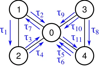
The real-world experiment used a network of ive IRIS wireless sensor nodes [12], set up in an oice environment and utilising the shared 2.4GHz ISM band. The topology of the network is described in Figure 1. A sixth IRIS node, connected to a PC over USB, was used to passively observe the network. The workload comprised eleven lows, which each represent a data transmission between tasks running on nodes, as described in Table 1.

In the real-world experiment no actual data was transmitted other than that required for the AirTight protocol. This results in actual transmissions which occur near instantaneously due to the minimal payload. Further, this means that ACKs contain a similar amount of data as the data frames, and thus take approximately the same amount of time to send as data frames.

The wireless nodes used in this experiment [12] feature an 8-bit micro-controller, limited storage and RAM. Somewhat problem-atically, the nodes also feature two clocks: a high-precision but low-duration timer used by the wireless communications hardware, and a low-precision but high-duration timer used by the operating system to schedule events. The dual timers are due to the fact that wireless communications require accurate timing to coordinate transmissions between nodes, but as these accurate transmissions are high-frequency and the nodes run on limited power, there is a trade-of between power usage and timing accuracy for higher frequency (i.e. < 10ms) events. Unfortunately, the dual clocks can cause issues; clock drift in the low-precision clock can be insignif-icant to the operating system, but may become signiinsignif-icant when measured by the high-precision clock. This represents an unfor-tunate inversion of the codiied methods of dealing with multiple levels of precision described by timebands [5], but is diicult to address without substantial modiication to the operating system. It will be shown that the clock synchronisation provides a signif-icant diference between the high-level simulator and real-world experiment. The techniques described in this paper allow these diferences to be attributed to speciic assumptions made by the high-level simulator.

However, while the issue of time synchronisation would nor-mally cause severe issues, it should be noted that in this experiment the utilisation of the wireless link was extremely low. This is due to the relatively small amounts of data being transmitted when compared to the slot size. Hence even if the wireless nodes transmit at inappropriate times, the chance of a collision is low.

This experiment provided information on approximately 65000 transmissions (sampled over approximately 1 day), which provides

0

1

2

3

4

τ

1

τ

7

τ

2

τ

4

τ

3

τ

11

τ

5

τ

6

[image:4.612.354.523.84.197.2]

τ

8

τ

10

τ

9

Figure 1: The network used in the real-world experiment

Name From To Criticality T D C P R

τ₁ n₁ n₂ _LO ₃₀ ₃₀ ₂ ₂ ₂₅

τ₂ n₁ n₀ _LO ₂₆ ₁₃ ₁ ₁ ₁₃

τ₃ n₂ n₀ _HI ₄₀ ₄₀ ₁ ₂ ₃₁

τ₄ n₂ n₀ _LO ₁₃ ₁₃ ₁ ₁ ₁₃

τ₅ n₀ n₄ _HI ₃₈ ₃₈ ₃ ₃ ₃₇

τ₆ n₀ n₄ _LO ₂₆ ₁₃ ₁ ₁ ₁₃

τ₇ n₀ n₁ _HI ₆₄ ₃₂ ₁ ₂ ₃₁

τ₈ n₃ n₄ _LO ₃₂ ₁₄ ₁ ₁ ₁₃

τ₉ n₃ n₀ _HI ₆₄ ₃₂ ₁ ₂ ₃₁

τ₁₀ n₃ n₀ _LO ₃₂ ₃₂ ₂ ₃ ₃₁

τ₁₁ n₄ n₀ _HI ₄₀ ₄₀ ₂ ₁ ₃₁

T_{: Period,}D_{: Deadline,}C_{: No of frames per packet,}P_{: Priority level,}

R_{: Response time,}τ_i_{: Flow}i

Table 1: Description of the Flows in the real-world experi-ment

adequate data to conduct a statistical investigation of the experi-ment. Further, the experiment also observed approximately 2000 faults, for which detailed information is available on 1100 by means of observing the efect of the faults on multi frame lows1. Hence this data allows us to characterise the behaviour of the faults in the real experiment.

3.2 Comparison of High Level Simulator and

Real-World Experiments

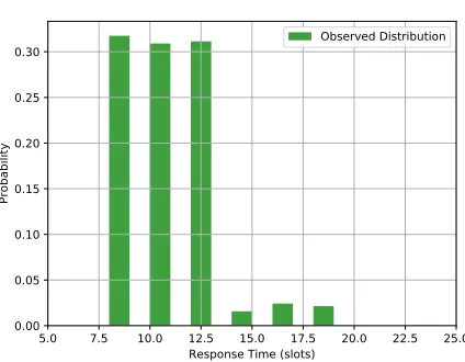
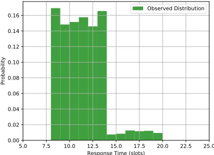
To motivate the issue of diferences between the real world ex-periment and the high level simulator, Figures 2 and 3 show the distribution of message response times for taskτ₉_{. As can be seen,} there are clear diferences between the two, with the most strik-ing diference bestrik-ing that the simulator only produces response times that are divisible by two. Ωhile omitted for space, similar diferences can be seen on the majority of other message lows. Interestingly, the AirTight slot table suggests that the simulated results are in fact valid, and that the phenomena observed in the real-world experiment is not the intended result.

Across all experiments, the following issues can be observed:

1_{The remaining 900 faults are only represented in frame retransmissions of single}

[image:4.612.322.557.235.392.2]

(5)

5.0 7.5 10.0 12.5 15.0 17.5 20.0 22.5 25.0 Response Time (slots)

0.00 0.02 0.04 0.06 0.08 0.10 0.12 0.14 0.16

Probability

[image:5.612.60.277.102.261.2]

Observed Distribution

Figure 2: Response times for real-world experiment for Flow

τ₉

0.00 0.05 0.10 0.15 0.20 0.25 0.30

Probability

Figure 3: Response times for high-level simulator for Flow

τ₉

(1) The High level simulator does not produce certain response times which are observed in the real-world experiment, which may lead to transmissions in the real-world experiment which are not observed in simulation.

(2) The real-world experiment can resend frames which were already successfully received and acknowledged, leading to more re-transmissions that what was observed in simulation.

(3) In the real-world experiment, expected frames (e.g. as part of a multi-frames sequence) can be completely absent, indi-cating the observer node is not recording all data.

Evidently there are diferences between the real experiment and the high-level simulator. However, there is very little compre-hension of why these diferences occur. In turn, this leads to the

possibility that these diferences relect laws in the high-level sim-ulator which lead to invalid results, a highly undesirable outcome. Hence it is prudent to examine why these diference may arise, by examining the assumptions made by the high level simulator.

4 VALIDATING THE HIGH-LEVEL

SIMULATOR RESULTS

In order to validate the high-level simulator results, and determine the reasons for the observered diferences, a low-level simulator will be used to explore the assumptions made by the high-level simulator. The low-level simulator used is parametrisable with respects to the major assumptions of the high-level simulator. This means that when run with all high-level simulator assumptions enabled, the low-level simulator matches the behaviour of the high-level simulator. However, these assumptions can be disabled, to bring the low-level simulator closer to the real-world experiments. Hence, by repeating the experiment in the low-level simulator under varying conigurations, and using statistics to compare the results of these conigurations with the high-level simulator and real-world experiments, a characterisation of the diferences be-tween the high-level simulator and real-world experiments can be obtained. This characterisation - the diference in conigurations of the low-level simulator - can then be used to argue whether or not the high-level simulator is suiciently accurate, and if not, the exact areas where accuracy should be improved.

4.1 Identifying High-level Simulator

Assumptions

In order to accomplish this, the irst step is to identify the assump-tions made by the high-level simulator [4]. In the previous work, only one assumption was tested: when the oline analysis deter-mined that a low assignment was schedulable, the high-level sim-ulator, which works at a protocol level, did not have any packets missing deadlines.

However, there are a number of assumptions that should be checked, as follows:

(1) Simulator is Observably Sound with respect to AirTight Analysis:The Simulator is assumed to be sound with re-spect to the oline analysis presented in [4] i.e. if the oline analysis deems a set of lows to be schedulable within certain deadlines, the simulator will not produce data that violates these deadlines. Independently, this assumption is also made of the real-world experiments.

(2) Slot Based Time:The high level simulator models time at the level of AirTight slots. Provided that clocks between nodes remain synchronised this is acceptable; however, if clock synchronisation starts to fail in an implementation, for example by the use of low precision clocks and interfer-ence impacting clock synchronisation messages, then this assumption may be invalid.

[image:5.612.62.274.327.492.2]

(6)

interference levels varying over time. Further, failures may have signiicant duration.

(4) Reciprocal Communication Ability:Due to the use of ACK it is obviously required that if node A communicates with node B, then node B must also be able to communicate with node A, but it may not be true that they can do so with equal success rates. However, the high level simulator assumes that for any link the failure rate is identical in both directions.

(5) Insigniicant interference of ACKs:The high-level simu-lator does not model ACKs in any meaningful capacity, which results in the high level simulator efectively assuming that all ACKs are successfully delivered. In practice however, an ACK failing to be delivered results in an unnecessary repeat transmission from the source node, a situation that cannot arise in the high level simulator. In the real experiment, due to the empty payload data frames and ACKs are of similar length, and hence could be assumed to have similar success and failure rates.

All of these assumptions are testable. Assumption 1 has been tested substantially in [4]; this work ran a large number of exper-iments in simulation and found no evidence that the simulator produced a result that contradicted the oline analysis. Further this was not observed in the real-world experiments, which suggests that the analysis is sound.

Assumption 2, that slot-based time is adequate for simulation can be made testable by means of a simulator that simulates time at a much more precise level. For this to be possible the state of each simulated node has to be modelled, and any clock drift in the low precision clocks of the nodes has to be part of the simulation.

Next, Assumption 3, that the failure rate of communications does not change over time, can be tested by modelling the failure rate of the real-world experiment. If a statistical distribution can be found that suiciently explains the observed data, then the assumption can be validated. If not, then this can be simulated by allowing the failure rate to vary over time in line with the real-world experiment. Assumption 4, that the failure rate of communications is constant over a link can be investigated by examining the failure rate of lows that travel in the opposite directions on a given physical link, and taking into account any temporal diferences indicated by the investigation into Assumption 3. For example,τ₂_andτ₇_{can be used} for this purpose.

Finally, Assumption 5 can be tested by investigating the rate of transmission and ACK failure in the real-world experiment. If it can be determined that ACK failure is a phenomenon that requires investigation, this can be simulated by allowing ACKs to be subject to interference.

Having identiied the additional simulation requirements, this paper now introduces a conigurable low-level simulator to char-acterise the diference between the high-level simulator and the real-world experiments.

4.2 Conigurable Low-Level Simulation

Ωhile using experimental data to validate the simulator is attractive from the point of view that the real-world experiment represents

a ªtrueº target for validation, using real hardware has many limi-tations. In particular, the nodes used in the experiment [12] have limited memory and storage, which makes obtaining detailed in-formation diicult. Hence a low-level simulator can be used as a validation target. Low-level simulators have a higher idelity view of the system they model2, but are computationally expensive to use and therefore undesirable for large scale or repeated experi-mentation.

This allows the extraction of far more information from the low-level simulator which can be used to determine the nature of any diferences from the high-level simulator. In turn, the low-level simulator can be validated against the real experiment, allowing any diferences between the high-level simulator and real experiment to be characterised accurately.

The conigurable low-level simulator used in this work makes far fewer absolute assumptions about the way wireless commu-nications behave than the high-level simulator. In particular, the low-level simulator allows:

• Non-uniform Time: To enable the modelling of clock

desyn-chronisation between wireless nodes. Used to test Assump-tion 2.

• Multiple Interference Models: To enable wireless

interfer-ence to be accurately calibrated to the real-world experiment. Used to test Assumption 3.

• Non-reciprocal Communications: To enable the modelling

of nodes which are not reliably able to communicate ACKs back to the source of a transmission. Used to test Assumption 4.

• ACK Transmission: To enable the determination of the

efects of ACK failure for retransmissions. Used to test As-sumption 5.

It is also important to note that each of these aspects can be conigured; in particular, this means that the low-level simulator can produce a collection of results allowing the impact of each aspect to be characterised. This allows the experiments to determine if any given aspect has a signiicant efect on the results of simulation, and hence informs if the high-level simulator could be signiicantly improved by modelling aspects of the real-experiment which when not modelled accurately (or at all) lead to substantial errors.

Unlike the high-level simulator, the low-level simulator is im-plemented by modelling each individual component of the system separately. This allows a much more in-depth simulation, at the ex-pense of signiicantly more computational efort than the high-level simulator, which can simply select the next packet to be simulated. The simulated components of the low-level simulator are as follows.

• Applicationswhich generate and receive application level

packets to transmit.

• MACwhich takes application level packets, encapsulates

them into network frames, and sends and receives these frames. The MAC layer also handles the sending and receiv-ing of ACKs, as well as retransmission.

• Physicalwhich takes network frames and models their

broadcast over the wireless network. This layer handles

2_{Note that the low-level simulator model is not identical to the real world system, due}

(7)

25 50 75 100 125 150 175 200 Fault Inter Arrival Time (slots)

0.00 0.01 0.02 0.03 0.04

Probability

[image:7.612.328.540.101.261.2]

Fitted Exponential Distribution Observed Distribution

Figure 4: Fault Inter-arrival times for the real-world experi-ment

whether or not an individual frame successfully transmits, and any potential collisions between frames.

It should be noted that the Application layer is typically not required to be updated as frequently as the MAC or Physical layers. This is simply due to the fact that the MAC and Physical layers pro-cess more data than the Application layer; even for Application data lows that it within a single network frame, an acknowledgement will normally be generated and must be processed.

4.3 Coniguring the Low-level Simulator

Ωhile most of the options for the low-level simulator are simple binary conigurations e.g. the choice to subject ACKs to interference or not, one option that needs more detailed coniguration is the wireless interference model. Hence this section details how this model is constructed using statistical observations from the real-world experiment.

There are two main properties to model for transmission failures: 1) the fault inter-arrival time, i.e. the characteristics of when faults arrive and 2) the fault durations i.e. the characteristics of how long faults persist. Further, these properties may vary for each physical link between nodes.

In the real-world experiment, interference on the wireless trans-missions can occur for a variety of reasons:

•Background noise

•Interference from external sources (e.g. oice equipment) •Transient hardware failure

Ωhile an interference model could be constructed for each packet low, the nature of the experiment where all nodes were positioned in close proximity on a desktop means that there is statistically insigniicant diference between each packet low. This manifests in the distributions of fault durations and fault inter-arrival times being identical for any packet lows, when comparing using the KS-test [16]. Hence it is possible to use a single global model in this case, although this may not be true more generally.

1 2 3 4 5 6 7 8 9

Fault Duration (slots) 0.0

0.2 0.4 0.6 0.8 1.0

Probability

[image:7.612.61.272.102.260.2]

Figure 5: Fault Durations for the real-world experiment

Even though the exact cause for any given fault cannot be known, it is still possible to use statistics to understand the characteristics of faults over time. This can be accomplished by assuming that faults are governed by an unknown random process, and all faults are independent of each other.

Using this assumption, faults can be modelled as being generated by a 1-dimensional Poisson Point Process [17]. However, this does not give the duration of faults, which is governed by a separate process which must be calibrated separately. This leads to the ob-servations that while fault durations are governed by the strength of the event, which can be an arbitrary distribution, the fault inter-arrival times are governed by an Exponential distribution [16]. This can be seen in Figure 4, where the fault inter-arrival times match very closely to the itted Exponential distribution. Further, while not shown this distribution is approximated by suiciently large contiguous subsections of the results, meaning that the fault inter-arrival times are governed by the same process throughout the experiment.

To inform the calibration of fault durations, Figure 5 shows the observations from the real world experiment. The vast majority of observed fault durations are of a single slot length, with the overall distribution being almost a single point. It can further be observed that the two slot faults observed can be explained by two single slot faults arriving in adjacent slots; the probability of faults arriving in two adjacent slots is 4%, which is the same probability as a fault of duration two. The lack of variability in fault durations trivially implies that the duration of a given fault is not temporally dependent.

For faults of length greater than two slots, there exists only a single longer fault of duration eight. As a singular event, it is not possible to understand this phenomena statistically. Outliers such as this may warrant further investigation, but this is beyond the scope of this work which focuses on statistical explanations.

Combining these observations, we can make the following obser-vations about transmission failures in the real-world experiment:

(8)

(2) Faults are instantaneous events which afect a single slot (3) Fault arrivals are governed by a Poisson Point Process (4) The characteristics of faults due to interference are constant

throughout the experiment

This information can then be used to construct a statistical inter-ference model for the low-level simulator which accurately relects the interference characteristics of the real-world experiment. In ad-dition, this also validates Assumption 2 for this experiment as there is no evidence that a temporally dependent process is impacting the faults.

5 EVALUATION

This section presents the results of the experiments carried out to check the assumptions of the simulator and how they difer from the real-world experiment. The experiments carried out were as follows.

(1) Real-world experiment (2) High-level simulator

(3) Low-level simulator with high-level simulator assumptions (4) Low-level simulator with calibrated interference model (5) Low-level simulator with calibrated interference model, ACK

failure and clock-drift

These experiments allow the impact of the various low-level conigurations to be determined with respect to the real-world and high-level simulator experiments. In turn, this allows the signii-cance of these changes to be correctly attributed.

5.1 Observations from Calibration

Firstly, we revisit the observation made during calibration that each physical wireless link has statistically identical fault inter-arival times and fault durations. This demonstrates that Assumption 4 holds for this experiment: There was no observable diference in the failure rate for each wireless link. Therefore it is valid to assume that for this experiment wireless communications are indeed reciprocal. This is likely due to the close physical proximity of the wireless nodes.

This also has a knock-on efect for the remaining experiments: as each physical link is identical, it is possible to use a global char-acterisation of the faults rather than a per-link charchar-acterisation. This simpliies the implementation of the remaining experiments, as well as enabling more data to be used to characterise the global link for greater accuracy. If Assumption 4 was shown not to hold it would be necessary to perform this characterisation of faults on each link, and potentially in each direction.

5.2 Low-level simulator with High-level

simulator assumptions

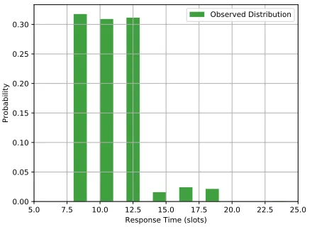
An important step is to verify that when the low-level simulator is conigured with high-level simulator assumptions, the low-level simulator replicates the results from the high-level simulator. This means coniguring the low-level simulator to experience zero trans-mission error, and all nodes have a global notion of time i.e. all clocks are in perfect synchronisation. These results can be seen in Figure 6, which shows the low-level simulator perfectly replicating

0.00 0.05 0.10 0.15 0.20 0.25 0.30

Probability

[image:8.612.324.544.102.262.2]

Figure 6: Response times for low-level simulator with high-level simulator assumptions for Flowτ₉

0.00 0.05 0.10 0.15 0.20 0.25 0.30

Pr

o

b

a

b

il

ity

[image:8.612.325.538.331.485.2]

Figure 7: Response times for low-level simulator with cali-brated interference model for lowτ₉

the results from the high-level simulator (Figure 3). This is true for all lows in this experiment.

This result allows us to attribute the diferences observed in the next experiments to the diferences in coniguration of the simulation. If such a coniguration also produces results which are comparable to real-world experiment, then the diference in coniguration can be used to explain the diference between the high-level simulator and the real-world experiment.

5.3 Impact of Interference Model

(9)

25 50 75 100 125 150 175 200 ACK Fault Inter Arrival Time (slots)

0.000 0.005 0.010 0.015 0.020 0.025 0.030 0.035 0.040

Probability

[image:9.612.58.273.101.260.2]

Figure 8: ACK failure inter-arrival distribution in real-world experiment

it is not suicient to accurately model the interference to explain the phenomena seen in the real-world experiment. It is therefore necessary to enable some of the additional simulation features of the low-level simulator.

5.4 Impact of ACK Failure

In order to investigate Assumption 5, ACK failures in the real-world experiment need to be monitored. Ωhile there is no direct method to observe ACK failures, they can be detected by examining the real-world experiment data for frames which were retransmitted despite being registered as received. This behaviour indicates that the sending node was not able to read the ACK, and hence chose to retransmit the frame. Analysing the results from the real-world experiment gives the inter-arrival distribution of ACK failures seen in Figure 8, which closely mirrors the distribution of transmission failures. As with transmission failure duration, ACK failure duration suggests that faults were instantaneous in nature, afecting only a single ACK. This is further bolstered by the fact that subsequent data transmissions do not have an increased chance of failure, suggesting that the duration of the interference that caused the ACK to fail is bounded by the time it takes to send the ACK.

Using the failure model of the real-world experiment, Figure 9 shows the ACK fault inter-arrival times for the low-level simulator. As can be seen, the low-level simulator is capable of matching the overall behaviour of ACK, with the same characterisation of the ACK fault inter-arrival times. This is in contrast to the high-level simulator, where ACK are assumed to succeed.

The impact of this on the validity of results from the high-level simulator is that the probability of failure used in the high-level sim-ulator does not necessarily relect the probability of a transmission failing in the real experiment. This is due to the fact that a single probability of failure used in the high level simulator has to account for two potential transmission failures i.e. the data transmission and the corresponding acknowledgement. Ωhile the individual

25 50 75 100 125 150 175 200 ACK Fault Inter Arrival Time (slots)

0.000 0.005 0.010 0.015 0.020 0.025 0.030 0.035 0.040

Probability

[image:9.612.323.539.103.260.2]

Figure 9: ACK failure inter-arrival distribution in the low-level simulator experiment with ACK failure

0.00 0.02 0.04 0.06 0.08 0.10 0.12 0.14 0.16

Probability

Figure 10: Results for low-level simulator with clock-drift

frame may still be delivered on time and the subsequent unnec-essary retransmission ignored, the very act of the retransmission has consequences. In multi-frame lows, the retransmission of an early frame may delay later frames. Further, retransmissions for any reason contribute to triggering high-criticality mode.

Therefore, when using the high-level simulator, the probability of failure must represent the combined probability of failure of data transmission and failure of acknowledgement. If naïvely using only the failure of data transmission, then the high-level simulator will not be a sound representation of the system, with multi-frame lows having shorter response times and the high-criticality mode being entered less frequently.

5.5 Impact of Clock Drift

[image:9.612.325.539.331.486.2]

(10)

Comparison of low-level simulator

Flow and real-world experiment

KS Test Metric Normalised Ωasserstein Metric

τ₁ _0.12 _0.03

τ₂ _0.15 _0.04

τ₃ _0.04 _0.07

τ₄ _0.10 _0.05

τ₅ _0.14 _0.04

τ₆ _0.19 _0.01

τ₇ _0.11 _0.01

τ₈ _0.10 _0.04

τ₉ _0.04 _0.01

τ₁₀ _0.18 _0.02

[image:10.612.63.286.83.237.2]

τ₁₁ _0.17 _0.02

Table 2: KS Test Metric and Normalised Wasserstein Met-ric comparing low-level simulator with clock drift and real-world experiment

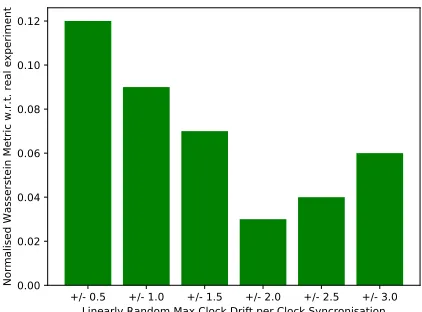
+/- 0.5 +/- 1.0 +/- 1.5 +/- 2.0 +/- 2.5 +/- 3.0 Linearly Random Max Clock Drift per Clock Syncronisation 0.00

0.02 0.04 0.06 0.08 0.10 0.12

Normalised Wasserstein Metric w.r.t. real experiment

Figure 11: Mean Normalised Wasserstein Metric for Clock Drift search

enabled. For this experiment, the parameters for the rate of clock-drift were searched for, with the mean error shown in Figure 11, and the best parameters found were to model clock-drift were a linear clock drift of between−2 and+2 slots per synchronisation. As can be seen, Figure 10 shows the characteristics of the real-world experiment, as seen in Figure 2. In particular, this includes

(1) Rare observations of response times faster than should be possible by analysis.

(2) Common observations of response times which should not occur according to analysis (for Figure 10, this includes all odd response times).

Comparing the results of the clock-drift low-level simulator and real-world experiment by means of the Kolmogorov-Smirnov (KS) test [16] provides evidence that the distributions are similar. This is corroborated with the normalised Ωasserstein Metric [13] which indicates the distributions are similar. These results for all lows are given in Table 2. A KS-test metric less than 0.19 indicates an accep-tance of the null hypothesis that the distributions are identical. The

Experiment Duration Duration (seconds)

Real hardware ≈1 Day ≈86400

Low-level simulator ≈1 Hour ≈3600

[image:10.612.324.550.83.127.2]

High-level simulator ≈2 Seconds ≈2

Table 3: Durations of the various experiments (simulations run on a Core i7-4500U laptop)

Ωasserstein Metric is a metric that indicates the diference between two empirical distributions; for ease of comparison this metric has been normalised with respect to the number and range of samples, where 0 indicates that distributions are identical and 1 indicates that the distributions are as diferent as possible. Hence these results suggest that clock-drift between nodes is a plausible explanation for the diferences between the real-world and high-level simulator. This conclusion can be made as the low-level simulator provides an exact match for the high-level simulator when running under the assumptions of the high-level simulator. However, when cali-brated for the interference model of the real-world experiment, the low-level simulator requires clock-drift in order to produce results that are comparable to the real-world experiment.

Fortunately, the amount of clock-drift is bounded due to the periodic resynchronisation of clocks provided by AirTight [4]. In the current experiment the relative sparseness of communications means the probability of simultaneous transmission is low, and so countermeasures are not necessary. In the event that wireless communications were more heavily used, it may be necessary to resynchronise the clocks of the wireless nodes more often, or use nodes that have higher precision time sources.

5.6 Analysis of Results

One of the main conclusions of these experiments is that while it is perfectly acceptable to design a protocol using a high-level simu-lation of that protocol, there can be unexpected behaviour when implementing the protocol on real hardware. The method used in this paper was able to identify multiple areas where assumptions of the high-level simulator caused diferences when compared to a real-world implementation, and was able to determine the major behavioural diferences were due to poor clock-synchronisation in the real-world experiment.

Even though the AirTight protocol provides periodic clock syn-chronisation [4], there is compelling evidence to suggest that the IRIS nodes used in the test implementation sufer from a signii-cant amount of clock drift. This can point to issues with either the hardware, or more likely, the use of the hardware by the implemen-tation of AirTight. However, none of the issues identiied fatally compromises the use of the high-level simulator. Instead, each issue can be mitigated; additional measurements can be taken to reine the probability of transmission failure to address the issues of ACK failure in the simulator, and higher degrees of clock synchronisa-tion can be used in the real hardware. Hence using the high-level simulator for protocol design remains a valid approach, provided that results are interpreted correctly.

[image:10.612.60.271.289.445.2]

(11)

in Table 3, the low-level simulator is an order of magnitude slower than the high-level simulator, which means it is inappropriate for any application where quick results are needed (e.g. search based methods for slot table selection). Further, the complexity of the low-level simulator scales linearly with the number of objects simulated, as opposed to the high-level simulator which simply selects the next step of the simulation based on the simulation description. This means that the low-level simulator is not useful for simulating more complex scenarios, such as the 25-node scenario demonstrated in [4].

Further, without calibration the low-level simulator produces results identical to the high-level simulator. If the real world en-vironment were to change, the low-level simulator would require recalibration for the results to be valid. Hence until the deployment environment of the system is known, it is arguable whether the results of the low-level simulator are any more accurate than those of the high-level simulator.

One can conclude that while the low-level simulator can indeed model the unusual behaviours of real-hardware more accurately than the high-level simulator, the high-level simulator is still appro-priate for exploring the behaviours of the AirTight protocol itself. However, translating results from simulation to a real implementa-tion can reveal unexpected behaviours which require explanaimplementa-tion that can easily be derived from the use of a low-level simulator.

Revisiting the assumptions of the high-level simulator, we can conclude the following:

(1) Simulator is Observably Sound with respect to AirTight Analysis:The experiments with the low-level simulator re-veal no evidence that the high-level simulator is unsound with respect to AirTight Analysis.

(2) Slot Based Time:Evidence was found that supports the idea that the nodes in the real-world experiment exhibited some amount of clock drift which explains why the real-world experiment observes response times which are not possible according to the transmission schedule. However, the abso-lute amount of clock drift appears to be small, causes low amounts of interference in the experiment, and is bounded. In the case that clock drift is signiicant, there are methods available that reduce the amount of clock drift.

(3) Temporally Uniform Interference:In the experiment anal-ysed, no evidence for temporally changing interference was uncovered. Further, by comparing multiple segments of an experiment it is possible to determine if this assumption is valid for any set of data.

(4) Reciprocal Communication Ability: By comparing all transmissions between nodes, no evidence to invalidate this assumption was found. Again, a method for determining if this assumption holds was outlined. If both this assumption and the previous assumption hold, it is suicient to only consider the global interference characteristics.

(5) Insigniicant interference of ACKs:Evidence was found that ACKs could fail; in so doing a small amount of additional work will be carried out by the transmitting node, which can potentially cause the real experiment to enter high-criticality mode before the high-level simulator would. This can be

addressed by setting the probability of transmission failure in the high-level simulator to account for both the failure of the data frame and its associated ACK.

6 SUMMARY AND CONCLUSIONS

This work has outlined and demonstrated a method for explain-ing the diferences between a high-level simulation and real world experiments by means of a conigurable low-level simulator and statistical understanding. Statistical methods allow the low-level simulator to mimic the behaviours observed in the real-world ex-periment, allowing phenomena that have been observed in the real-world experiment to be explored thoroughly. This coniguration of the low-level simulator can then be compared to a coniguration that replicates the results of the high-level simulator in order to attribute the diferences of the high-level simulation and real-world experiments to speciic coniguration changes.

Attributation of diferences in the high-level simulator and real-world experiments allows a user to understand why a simulation difers from reality. In turn, this allows for either targeted improve-ments to be made to the high-level simulator or a simple explanation of why the diference does not warrant concern.

The statistical method used in this paper has limitations with respect to anomalous events, because by their nature anomalous events do not provide suicient data to be statistically characterised. However, anomalous events are detectable by the methods used, as they are unexplained by the statistical models selected. The detection of anomalous events informs the user of the method and allows them to decide if the anomalous events should be discarded (on the grounds that they are suiciently rare as to not impact a deployment of the system) or if further experimentation and attempts to reproduce the anomalous events should be conducted. These techniques have been illistrated by investigating the dif-ference between the high-level simulator described in [4] and the real world experiments, and how these diferences can be mitigated. This has also illustrated that even though more accurate results can be found with the conigurable low-level simulator deined in this paper, the fact that the high-level simulator requires much lower computational efort (by a factor of over 1000) means that it is more useful for developing the AirTight protocol. However it is possible that some features, for example automatic calculation of transmission interference probability given the probability of a frame transmission failure and ACK transmission failure could be added to the high-level simulator to increase its accuracy.

(12)

ACKNOWLEDGEMENTS

The research described in this paper is funded, in part, by the EPSRC grant MCCps (EP/P003664/1). No new primary data were created during this study.

REFERENCES

[1] IEEE standard for information technologyś local and metropolitan area networksś speciic requirementsś part 3: CSMA/CD access method and physical layer speciications amendment 4: Media access control parameters, physical lay-ers, and management parameters for 40 gb/s and 100 gb/s operation. IEEE Std 802.3ba-2010 (Amendment to IEEE Standard 802.3-2008), pages 1ś457, June 2010.doi:10.1109/IEEESTD.2010.5501740.

[2] R. Baheti and H. Gill. Cyber-physical systems.The impact of control technology, 12(1):161ś166, 2011.

[3] S. Bullock and E. Silverman. Levins and the legitimacy of artiicial worlds. In N. David, editor,Third Workshop on Epistemological Perspectives on Simulation, 2008. URL: http://eprints.ecs.soton.ac.uk/16778/.

[4] A. Burns, J. R. Harbin, L. S. Indrusiak, I. Bate, R. I. Davis, and D. Griin. Airtight: A resilient wireless communication protocol for mixed-criticality systems. In

IEEE Embedded and Real-Time Computing Systems and Applications, 6 2018. [5] A. Burns and I. J. Hayes. A timeband framework for modelling real-time systems.

Real-Time Systems, 45(1-2):106ś142, 2010.

[6] N. Hillary and K. Madsen. You can’t control what you can’t measure, or why it’s close to impossible to guarantee real-time software performance on a CPU with on-chip cache. In2nd International Workshop On Worst-Case Execution Time Analysis, pages 45ś48, Technical University of Vienna, Austria, June 2002.

[7] K. Jain, J. Padhye, V. N. Padmanabhan, and L. Qiu. Impact of interference on multi-hop wireless network performance.Wireless networks, 11(4):471ś487, 2005. [8] P. Levis, N. Lee, M. Ωelsh, and D. Culler. Tossim: Accurate and scalable simulation of entire tinyos applications. InProceedings of the 1st international conference on Embedded networked sensor systems, pages 126ś137. ACM, 2003.

[9] T. H. Lim.Dependable Network Protocols in Wireless Sensor Networks. PhD thesis, University of York, 2013.

[10] A. Maskooki, C. B. Soh, E. Gunawan, and K. S. Low. Adaptive routing for dynamic on-body wireless sensor networks.IEEE Journal of Biomedical and Health Informatics, 19(2):549ś558, March 2015.doi:10.1109/JBHI.2014.2313343. [11] T. Mehmood. COOJA network simulator: Exploring the ininite possible ways to

compute the performance metrics of IOT based smart devices to understand the working of IOT based compression and routing protocols, 2017.arXiv:arXiv: 1712.08303.

[12] Memsic. IRIS wireless measurement system. http://www.memsic.com/useriles/ iles/Datasheets/ΩSN/IRIS_Datasheet.pdf.

[13] Y. Rubner.International Journal of Computer Vision, 40(2):99ś121, 2000. URL: https://doi.org/10.1023/a:1026543900054,doi:10.1023/a:1026543900054. [14] S. Safaric and K. Malaric. Zigbee wireless standard. InProceedings ELMAR 2006,

pages 259ś262, June 2006.doi:10.1109/ELMAR.2006.329562.

[15] R. G. Sargent. Veriication and validation of simulation models. InSimulation Conference (WSC), Proceedings of the 2009 Winter, pages 162ś176. IEEE, 2009. [16] L. J. Stephens.Schaum’s Outlines: Beginning Statistics. McGraw-Hill, 2nd edition,

2006.

[17] D. Stirzaker. Advice to hedgehogs, or, constants can vary.The Mathematical Gazette, 84(500):197ś210, 2000. URL: http://www.jstor.org/stable/3621649. [18] S. Vestal. Preemptive scheduling of multi-criticality systems with varying degrees