Distributed parallel cooperative coevolutionary multi-objective large-scale immune algorithm for deployment of wireless sensor networks

(1)

This is a repository copy of

Distributed parallel cooperative coevolutionary multi-objective

large-scale immune algorithm for deployment of wireless sensor networks

.

White Rose Research Online URL for this paper:

http://eprints.whiterose.ac.uk/150774/

Version: Accepted Version

Article:

Cao, B., Zhao, J., Yang, P. orcid.org/0000-0002-8553-7127 et al. (6 more authors) (2018)

Distributed parallel cooperative coevolutionary multi-objective large-scale immune

algorithm for deployment of wireless sensor networks. Future Generation Computer

Systems, 82. pp. 256-267. ISSN 0167-739X

https://doi.org/10.1016/j.future.2017.10.015

Article available under the terms of the CC-BY-NC-ND licence

(https://creativecommons.org/licenses/by-nc-nd/4.0/).

[email protected] https://eprints.whiterose.ac.uk/

Reuse

This article is distributed under the terms of the Creative Commons Attribution-NonCommercial-NoDerivs (CC BY-NC-ND) licence. This licence only allows you to download this work and share it with others as long as you credit the authors, but you can’t change the article in any way or use it commercially. More

information and the full terms of the licence here: https://creativecommons.org/licenses/

Takedown

If you consider content in White Rose Research Online to be in breach of UK law, please notify us by

(2)

Distributed Parallel Cooperative Coevolutionary Multi-Objective Large-Scale Immune

Algorithm for Deployment of Wireless Sensor Networks

Bin Caoa,b,c,∗

, Jianwei Zhaoa,b,c_{, Po Yang}d,∗

, Zhihan Lve_{, Xin Liu}f_{, Xinyuan Kang}a,b,c_{, Shan Yang}a,b,c_{, Kai Kang}f_{, Amjad}

Anvari-Moghaddamg

a_{School of Computer Science and Engineering, Hebei University of Technology, 300401 Tianjin, China} b_{Key Laboratory of Machine Intelligence and Advanced Computing, Ministry of Education, 510006 Guangzhou, China}

c_{Hebei Provincial Key Laboratory of Big Data Calculation, 300401 Tianjin, China} d_{Department of Computer Science, Liverpool John Moores University, Liverpool, UK}

e_{School of Data Science and Software Engineering, Qingdao University, 266071 Qingdao, China.} f_{Hebei University of Technology, 300401 Tianjin, China.}

g_{Department of Energy Technology, Power Electronic Systems, 9220 Aalborg, Denmark.}

Abstract

The use of immune algorithms is generally a time-intensive process—especially for problems with numerous variables. In the present paper, we put forward a distributed parallel cooperative coevolutionary multi-objective large-scale immune algorithm that is implemented using the message passing interface (MPI). The proposed algorithm comprises three layers: objective, group and individual layers. First, to address each objective in a multi-objective problem, a subpopulation is used for optimization, and an archive population is used to optimize all the objectives. Second, the numerous variables are divided into several groups. Finally, individual evaluations are allocated across many core processing units, and calculations are performed in parallel. Consequently, the computation time is greatly reduced. The proposed algorithm integrates the idea of immune algorithms, which explore sparse areas in the objective space, and uses simulated binary crossover for mutation. The proposed algorithm is employed to optimize the 3D terrain deployment of a wireless sensor network, which is a self-organization network. In our experiments, through compar-isons with several state-of-the-art multi-objective evolutionary algorithms—the cooperative coevolutionary generalized differential evolution 3, the cooperative multi-objective differential evolution, the multi-objective evolutionary algorithm based on decision vari-able analyses and the nondominated sorting genetic algorithm III—the proposed algorithm addresses the deployment optimization problem efficiently and effectively.

Keywords: decision variable analysis (DVA), cooperative coevolution (CC), large-scale optimization, message passing interface (MPI), wireless sensor networks (WSNs), 3D terrain deployment

1. Introduction

In the wireless sensor network (WSN) deployment optimiza-tion procedure [1], wireless sensor nodes can be optimized via self-organization [2] to maximize the Coverage, optimize the

Connectivity Uniformity and minimize the Deployment Cost.

With the rapid development of sensor and wireless communi-cation technologies, WSNs have been applied to various fields. The work of [3] presented an air temperature monitoring appli-cation for WSNs. Shen et al. [4] described the wireless sensor nodes for a medical service. Zhang et al. [5] illustrated the WSN k-barrier coverage problem. Zhou et al. [6] researched the energy issue, regarding which clustering and data compres-sion were studied. Zhang et al. [7] utilized mobile sinks to alleviate the communication burden.

In addition, the response of the human immune system to antigens can be viewed as a process of self-organization.

∗_{Corresponding authors.}

E-mail addresses: [email protected] (Po Yang), [email protected] (Bin Cao)

Based on this concept, the clonal selection algorithm (CLON-ALG) [8], which can be used for global optimization problems (GOPs) and multi-objective optimization problems (MOPs) [9], was proposed. Other nature-inspired algorithms also follow the self-organizing procedure. For example, Xue et al. [10] de-scribed the self-adaptive artificial bee colony algorithm, which is different from the immune algorithm.

In the real world, many problems require several (usu-ally conflicting) objectives to be considered simultaneously. Multi-objective evolutionary algorithms (MOEAs) [11, 12, 13] are capable of producing a plurality of solutions during one run, which is convenient for approximating the Pareto front (PF). For NP-hard problems, evolutionary algorithms (EAs) [14, 15, 16, 17] can usually converge to near-optimal solutions using limited computational resources [18] within a reasonable time compared to brute force and deterministic methods.

(3)

se-lects a small quantity of nondominated individuals in a sparse area for cloning, recombination and mutation. In [21], sim-ulated binary crossover (SBX) and differential evolution (DE) were combined and applied to cloned individuals in a hybrid evolutionary framework for MOIAs called HEIA, which per-formed well for both unimodal and multimodal problems.

EAs are based on an iterative evolution of the population (the solutions), which is time-consuming—especially for ex-pensive problems. Distributed evolutionary algorithms (dEAs) [22, 23] allocate the tedious computational burden across nu-merous computational nodes, greatly reducing the required time. Cloudde [24] used DEs with various parameters to op-timize multiple populations in a distributed parallel manner, yielding a promising performance from both the effect and effi -ciency aspects. [25] provided a comprehensive study concern-ing parallel/distributed MOEAs. Utilizing the multi-objective optimization algorithm based on decomposition (MOEA/D) [13], parallel MOEA/Ds (pMOEA/Ds) [26] [27] were pro-posed.

With the arrival of “big data”, many complex problems have emerged; solving such problems is both time-consuming and storage-consuming [28, 29]. Similarly, many MOPs now have numerous variables (e.g., more than 100 variables [30]). Some examples include classification [31], clustering [32], and rec-ommendation systems [33]. However, the goal of traditional MOEAs is to solve multi-objective small-scale optimization problems (MOSSOPs). Consequently, the traditional algo-rithms may be incapable of tackling multi-objective large-scale optimization problems (MOLSOPs) because of the “curse of di-mensionality”. To optimize numerous variables, some promis-ing approaches first separate the variables into groups and then optimize them in a cooperative coevolutionary (CC) [34] man-ner. For large-scale global optimization problems (LSGOPs), many grouping mechanisms have been applied, including fixed grouping [34], random grouping [35], the Delta method [36], dynamic grouping [37], differential grouping (DG) [38], global differential grouping (GDG) [39] and graph-based differential grouping (gDG) [40]. Antonio et al. proposed the cooperative coevolutionary generalized differential evolution 3 (CCGDE3) method [41], which used fixed grouping.

MOLSOPs differ from LSGOPs in that no single solution optimizes all the conflicting objectives; instead, a solution set should be generated to approximate the PF. In MOLSOPs, vari-ables have different properties [42], which can be classified as follows:

1. position variables, which affect only the diversity of the solution set;

2. distance variables, which affect only the convergence of the solution set; and

3. mixed variables, which affect both the diversity and the convergence of the solution set.

Therefore, position variables should be permuted to approxi-mate the PF as comprehensively as possible. However, distance variables should be optimized so that they can closely approach the PF.

To identify these variable types, the multi-objective evo-lutionary algorithm based on decision variable analyses (MOEA/DVA) [30] utilizes a mechanism called decision vari-able analyses (DVA). The position as well as mixed varivari-ables are categorized as diversity-related variables, while distance variables, as related variables. The convergence-related variables are allocated to multiple groups that are then optimized under the CC framework.

The use of multiple populations can impact the optimization performance. In cooperative multi-objective differential evolu-tion (CMODE) [43], each objective is optimized by a subpop-ulation, and an archive is used to maintain good solutions and optimize all objectives. This approach has yielded good exper-imental results.

Compared to MOSSOPs, designing parallel/distributed MOEAs for MOLSOPs will be more beneficial. In this pa-per, we propose the distributed parallel cooperative coevolu-tionary multi-objective large-scale immune algorithm (DPCC-MOLSIA), which is aimed at solving MOLSOPs effectively and efficiently.

The contributions of this paper can be summarized as fol-lows:

1. Each objective is optimized by a subpopulation. Thus, the exploration with respect to each objective is enhanced, and all objectives are comprehensively optimized by an archive. Variables are grouped according to their prop-erties and interactions, contributing to effective optimiza-tion.

2. The idea of the IA is introduced, more computational re-sources are used to explore sparse areas in the objective space, andSBXis utilized for evolution.

3. We construct a three-layer parallel structure. The evalu-ations of individuals in different groups of multiple pop-ulations can then be performed in parallel, which greatly reduces the computation time.

The remainder of this paper is organized as follows: Sec-tion 2 provides some preliminary informaSec-tion required for this paper. The details of the DPCCMOLSIA are discussed in Sec-tion 3. Then, in SecSec-tion 4, we describe the experimental study and present the corresponding analyses. Finally, Section 5 con-cludes this paper.

2. Preliminaries

2.1. MOP and Variable Properties

An MOP involves several objectives that usually conflict with each other. Therefore, addressing an MOP comprises obtaining a solution set that approximates the PF. For the minimization problem, we have the following formula:

MinimizeF(X)={f1(X),f2(X), ...,fM(X)}, (1)

whereX=(X1,X2, ...,XD) is a point in the solution spaceℜD.

Here,Ddenotes the variable quantity, fi,i=1,2, ...,M,

repre-sents the objectives, andF(X) denotes the point in the objective spaceℜM

(4)

f₁(x)

1 1.5 2 2.5 3

f2

(x)

-0.5 0 0.5 1 1.5 2 2.5

Only altering x₁ Only altering x₂ Only altering x

3

[image:4.595.303.560.87.493.2]

Only altering x₄ Only altering x₅

Figure 1: Image of solution sets for the MOP formulated in Eq. 2, sampled by altering one variable while holding the others constant at 0.5.

Due to the conflicts among objectives, the types of different variables involved can be numerous; correspondingly, variables can be classified as position, distance, and mixed variables. For instance, consider the following MOP:

(

f1=0+x1+sin (4πx2)+ex3(x4−0.05)+x25

f2=1−x1−cos (4πx2)+x23+x 3

4+x

2 5

s.t.xi∈[0,1], i=1,2,3,4,5,

(2)

where f1and f2are two objectives andx1,x2,x3,x4andx5are

decision variables.

Fig. 1 illustrates the solution sets sampled by altering each variable individually while holding the others constant at 0.5. From the image, we can determine the properties of the vari-ables: x1is a position variable, as it influences only the

diver-sity; x2 is a mixed variable, as it influences both the diversity

and the convergence; x3 andx4are distance variables, though

their relative positions change only slightly with variation of the values; and x5 is a distance variable, as it influences only

the convergence.

2.2. CC

CC [34] divides a great quantity of variables into several sub-components that are optimized separately. For fitness evalua-tion, the target subcomponent is recombined with representa-tives from the other components to constitute a complete solu-tion.

2.3. Immune Algorithm

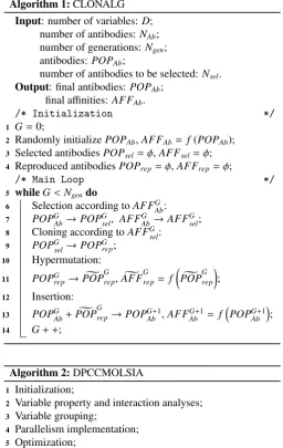
The CLONALG was proposed in [8]; its process is detailed in Algorithm 1. In the CLONALG, anantibodydenotes a

can-Algorithm 1:CLONALG

Input: number of variables:D; number of antibodies: NAb;

number of generations:Ngen;

antibodies:POPAb;

number of antibodies to be selected: Nsel.

Output: final antibodies:POPAb;

final affinities:AFFAb.

/* Initialization */

1 G=0;

2 Randomly initializePOPAb,AFFAb= f(POPAb);

3 Selected antibodiesPOPsel=φ,AFFsel=φ;

4 Reproduced antibodiesPOPrep=φ,AFFrep=φ;

/* Main Loop */

5 whileG<Ngendo

6 Selection according toAFFG

Ab:

7 POPG

Ab→POP G sel, AFF

G

Ab→AFF G sel;

8 Cloning according toAFFG_sel: 9 POPG_sel→POPG_rep;

10 Hypermutation: 11 POPG_rep→POPg

G rep,AFFg

G rep= f

g

POPG_rep

;

12 Insertion: 13 POPG_Ab+POPg

G

rep→POP G+1

Ab ,AFF G+1

Ab = f

POPG_Ab+1;

14 G+ +;

Algorithm 2:DPCCMOLSIA

1 Initialization;

2 Variable property and interaction analyses; 3 Variable grouping;

4 Parallelism implementation; 5 Optimization;

didate solution, the optimal solution is seen as theantigen, and theaffinityrepresents the fitness.

3. The Proposed Algorithm: DPCCMOLSIA

Algorithm 2 lists the main steps in the framework of the DPCCMOLSIA. The main procedure is detailed in the follow-ing subsections.

3.1. Variable Property and Interaction Analyses

Variables are classified as position variables, distance vari-ables and mixed varivari-ables according to their influences on di-versity and convergence. At the end of this process, the posi-tion variables and mixed variables are categorized as diversity-related variables, and the distance variables are categorized as convergence-related variables. For the MOP formulated in Eq. 2, x1 andx2 are classified as diversity-related variables, while

[image:4.595.48.268.93.317.2]

(5)

3.2. Variable Grouping

Because more than one objective exists, the interactions among variables are obtained with respect to each objective by adopting the idea of gDG [40]. The diversity-related variables are separated into a single group. We group the convergence-related variables according to the following idea: if two vari-ables interact with each other for any objective optimized in the present subpopulation/archive, we consider them to be interact-ing. Take the MOP mentioned above in Eq. 2 for example,

x1andx2are diversity-related variables; thus, they are grouped

together. For the convergence-related variables, x3and x4

in-teract in f1and act independently in f2; thus, we allocate them

to a single group in subpopulation 1 (only optimizing f1), to

separate groups in subpopulation 2 (only optimizing f2), and to

the same group in the archive (optimizing both f1and f2).x5is

independent from other variables for both f1and f2; thus, it is

allocated to another separate group.

3.3. Parallelism Implementation

For MOLSOPs, especially expensive ones, parallelism can be beneficial. The DPCCMOLSIA is a distributed parallel al-gorithm implemented using the MPI. In the DPCCMOLSIA, the parallel structure has three layers.

Assuming thatNCPU _{CPU resources are available, the}

vari-ables are divided into N_iGgroups. Here, i = 1,2, ...,M+1— the subpopulations are represented by i = 1,2, ...,M, and the archive is represented by i = M+1. NPindividuals exist in each subpopulation and in the archive population. Then, we have the following equation:

NCPU

i =

NG i

PM+1

j=1 NGj

×NCPU

s.t.i=1,2, ...,M+1,

(3)

whereN_iCPUdenotes the quantity of CPUs allocated to the sub-populationior the archive.

NCPU

i,j =

NCPU

i

NG i

s.t. j=1,2, ...,NG i ,

(4)

whereNCPU_i_,_j is the quantity of CPUs in the charge of group jin subpopulationior the archive.

The evaluations of the individuals are allocated across the multiple CPUs in each group.

N_iCPU_,_j_,_k = NP

NCPU

i,j

s.t.k=1,2, ...,N_iCPU_,_j ,

(5)

whereNCPU

i,j,k is the number of individuals that are assigned to

CPUkof group jin subpopulationior the archive.

Therefore, based on the three-layer parallel structure, the evaluations of the individuals in each group of allM+1 pop-ulations are conducted in parallel, which substantially reduces the computation time.

To guarantee the optimization performance, information must be shared among the groups. Hence, the communication

Algorithm 3:Evolution

Input: generation number:Ngen.

Output: final population: POPf inal.

1 forG=1→Ngendo

2 Evolve all variable groups in the subpopulations

(Algorithm 4) and the archive (Algorithm 5) in parallel;

3 Exchange information among the groups;

4 Gather all the individuals from all groups to generate the

final populationPOPf inal;

strategy should be properly designed [44, 45]; we adopt the von Neumann topology.

3.4. Evolution Combined with the Idea of the IA

The overall evolution process is provided by Algorithm 3. The evolution of each group in the subpopulations (Algorithm 4) or in the archive (Algorithm 5) is described in the following subsections.

3.4.1. Subpopulations

In Line 2 of Algorithm 4, in the evolution, tour selection is employed to choose 2 individuals from the full population. Then, in Lines 3 and 4, we useSBXto evolve variables in the target group and integrate them with other variables to form a complete individual.

e

Xi,j=

(

S BX Xi,Xr1,Xr2,j

if j∈index

Xr3,j otherwise, (6)

whereXei denotes the generated new solution, Xi is the target

parent individual, Xr1 andXr2 are the 2 reference individuals,

Algorithm 4:Evolution of One Variable Group in Subpop-ulations

Input: number of individuals:NP; population: POP1.

Output: new population:POPnew1.

/* Evolution */

1 fori=1→NPdo

2 Select 2 reference individuals; 3 UseSBXto generate offspringi;

4 Combine the generated offspring with other variables

to construct a complete solution;

5 Performpolynomial mutation;

/* Evaluation */

6 Allocate the generated solutions to the CPU resources in

the group and perform the evaluations in the CPUs in parallel;

7 Collect the fitness values from the CPUs;

/* Refinement */

8 Combine the generated solutions with the old population; 9 ObtainNPindividuals with respect to their fitness values

(6)

index contains the variables to be optimized by the present group, andXr3is integrated with the optimized variables to form

a complete solution, which has the following form:

r3 =

    

i ifr< G

Ngen

r4 else ifr′<0.5

r5 otherwise,

(7)

whereGdenotes the present generation number and Ngen

de-notes the maximum generation number. Here,randr′are ran-dom numbers generated uniformly within [0.0,1.0], andr4and

r5are two individuals selected via tour selection. Then, in Line

5,polynomial mutationis performed.

In Lines 6 and 7, to evaluate the newly generated solutions, we use parallelism to alleviate the computational burden. This is the third layer of the parallel structure of the DPCCMOLSIA. Finally, in Lines 8 and 9, theNPbest individuals with respect to the considered objective are preserved.

3.4.2. Archive

Traditionally, in each generation, all individuals take part in evolution. However, this paper introduces the idea of the IA, in which, in each generation, we select several good individuals and produceNPoffspring, the entire process of which is illus-trated in Algorithm 5. In detail, the selection of individuals in Line 1 is determined by two criteria: nondominance and crowd-ing distance. If the quantity of nondominated individuals is less thanNsel, all of them are selected for cloning; otherwise, we

se-Algorithm 5:Evolution of One Variable Group in Archive

Input: number of individuals:NP; population:POP2;

maximum number of individuals to be selected:Nsel.

Output: new population:POPnew2.

/* Selection */

1 SelectN_selindividuals according to the Pareto dominance

and crowding distance;

/* Clone */

2 Clone the selected individuals to a total number ofNP;

/* Evolution */

3 fori=1→NPdo

4 Select 2 reference individuals; 5 UseSBXto generate the offspringi;

6 Combine the generated offspring with other variables

to construct a complete solution;

7 Performpolynomial mutation;

/* Evaluation */

8 Allocate the generated solutions to the CPU resources in

the group and perform evaluations on the CPUs in parallel;

9 Collect the fitness values from the CPUs;

/* Nondominated sorting */

10 Combine the generated solutions with the old population; 11 ObtainNPindividuals according to the Pareto dominance

and crowding distance→POPnew2;

lect theNselindividuals that have larger crowding distances. In

the cloning process in Line 2, the quantity of replicates of each selected individual depends on the crowding distance [21].

NC_i =_P_Ndisti

sel

j=1distj

×NP, ₍₈₎

whereNC

i represents the number of replications of selected

in-dividuali anddistiis its crowding distance in the population,

which is calculated as follows:

disti= M

P

m=1

distm

i , (9)

wheredistm

i denotes the crowding distance of thei-th individual

with respect to objectivem, with

distm_i =     

∞ if (i)∗=1

0 if (i)∗=NP

e

fm(i)∗+1−ef

(i)∗₋₁

m

e

fNP m −efm1

otherwise.

(10)

e

fm(i)∗ is the fmi sorted in descending order, and (i)

∗

denotes the new index of thei-th individual in the sorted sequence.

disti=

(

2×distmax

i ifdisti=∞

disti otherwise, (11)

wheredistmax

i is the maximum crowding distance. Because∞

values are assigned to the crowding distances, to calculateNC i ,

we have to convert them.

In Line 4 of the evolution process, we select 2 individuals from among theNselselected individuals ifNsel>2; otherwise,

the selection scope is the whole population. Then, in Lines 5 and 6, we useSBXto generate the target individual. For the in-tegration,r4andr5(Eq. 7) are 2 randomly selected individuals

from theNselbest individuals used for cloning when Nsel >2

or from the whole population whenNsel ≤2. Then, in Line 7,

polynomial mutationis performed.

Finally, in Lines 10 and 11, we combine the new individu-als with the present population to obtain theNPbest individu-als according to the Pareto dominance and crowding distance. When the quantity of nondominated individuals is belowNP, several dominated individuals will be preserved.

4. Experimental Research: Application to 3D Terrain De-ployment of Heterogeneous Directional Sensor Networks

4.1. 3D Deployment Problem and Terrain Data

We use the 3D deployment problem proposed in [1], which includes three objectives: Coverage, Connectivity Uniformity

(7)

(a) Plain Terrain (b) Hilly Terrain (c) Mountainous Terrain

Figure 2: Illustration of 3D terrain data.

4.2. Parameter Setup

We compare the DPCCMOLSIA with the CCGDE3 [41], the CMODE [43], the MOEA/DVA [30] and the nondominated sorting genetic algorithm III (NSGA-III) [46] in terms of ad-dressing the deployment optimization problem.

For all the algorithms, the optimization process is performed 24 times. The fitness evaluations (FEs) are set to 104_×_D_{; here,}

D=2×102_.

To ensure fair comparison, we set the population size, NP, to 120 with respect to all algorithms. Specifically, for the CCGDE3, the population is split into 2 subpopulations, each of which has 60 individuals. For CMODE, because there are 3 ob-jectives that must be optimized, we use 3 subpopulations, each of which has 20 individuals, and set the maximum size of the archive to 120. For the MOEA/DVA and NSGA-III, we simply setNPto 120. For the DPCCMOLSIA, each of the subpopu-lations and the archive population has 120 individuals. Finally, we select 120 individuals from all populations.

DEis used in the CCGDE3, and we setF =0.5 andCR =

1.0.SBXandpolynomial mutationare used in the MOEA/DVA, NSGA-III and DPCCMOLSIA, and the distribution indexes are set toηc =ηm=20. The probabilities of crossover and

muta-tion are set topc=1.0 andpm=1.0/D, respectively.

For MOEA/DVA, the probability of selecting individuals among the neighborhood is 0.9, the neighborhood size is 0.1×

NPand the replace limit is 0.01×NP.

For DVA in MOEA/DVA, the number of control variable analysis isNCA=20 and the number of interdependence anal-ysis isNIA=6. For the variable property and interaction anal-yses in DPCCMOLSIA,NCA=20 andNIA=1.

Additionally, for the DPCCMOLSIA, we setNsel=0.1×NP,

and the number of CPUs used is 72, while other algorithms are serial.

4.3. Performance Indicator

Because the optimal solutions are unknown, we use the hy-pervolume (HV) indicator [47] and visualize all the obtained solution sets. The HV indicator translates the solution set qual-ity into a single evaluation index. The higher the HV indicator value, the better the optimization performance.

4.4. Results and Analyses

1 0.8 0.6

Coverage 0.4 0.2 0 0 0.05 Uniformity

0.1 0.15 0.2 0 0.1 0.2 0.3 0.4 0.5 0.6

0.25

Cost

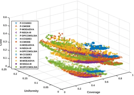
[image:7.595.324.541.471.624.2]

P-CCGDE3 P-CMODE P-MOEA/DVA P-NSGA-III P-DPCCMOLSIA H-CCGDE3 H-CMODE H-MOEA/DVA H-NSGA-III H-DPCCMOLSIA M-CCGDE3 M-CMODE M-MOEA/DVA M-NSGA-III M-DPCCMOLSIA

Figure 3: Visualization of solutions for all terrains. First, we demonstrate all the obtained final nondominated so-lutions after 24 runs of each algorithm on each of the three ter-rains in Fig. 3. Here,P− ∗denotes the results for the plain terrain,H− ∗denotes the results for the hilly terrain, andM− ∗

denotes the results for the mountainous terrain.

(8)

terrain, the algorithms tend to perform well in terms of the De-ployment Costobjective. Finally, for the mountainous terrain, the performances of the algorithms are far inferior to their per-formances for the other two terrains. We can comment on the above phenomena as follows:

1. Because the plain terrain is flatter than the other two ter-rains, it is easier to achieve betterCoverage.

2. The hilly terrain has fluctuations in elevation, and the algo-rithms tend to deploy the sensor nodes in low-lying areas, thus guaranteeing betterDeployment Cost.

3. The mountainous terrain has severe elevation changes, which makes it much more difficult to address compared with the other two terrains. Consequently, the algorithms exhibit poor performances for this terrain.

In the following, we give detailed results of all algorithms with respect to each terrain and provide corresponding perfor-mance analyses.

4.4.1. Plain Terrain

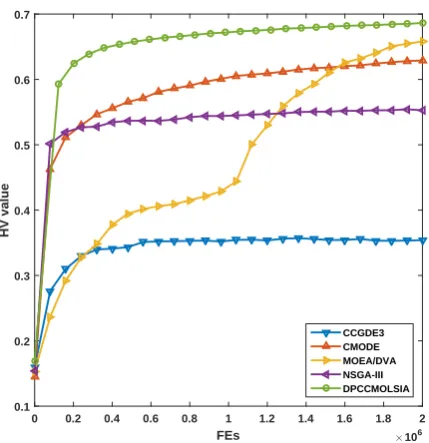
The evolutionary curves of the HV indicator values are illus-trated in Fig. 4.

We can see that the DPCCMOLSIA has the best perfor-mance (0.6864839), followed by the MOEA/DVA (0.6582590), the CMODE (0.6290526), and the NSGA-III (0.5526697); the CCGDE3 has the worst performance (0.3539973). Moreover, the DPCCMOLSIA has the fastest convergence speed, but less improvement occurs in the consequent process, while the MOEA/DVA is quite inferior in the beginning stage but im-proves significantly in the middle stage.

FEs ×106

0 0.2 0.4 0.6 0.8 1 1.2 1.4 1.6 1.8 2

HV value

0.1 0.2 0.3 0.4 0.5 0.6 0.7

[image:8.595.360.500.79.745.2]

CCGDE3 CMODE MOEA/DVA NSGA-III DPCCMOLSIA

Figure 4: Evolutionary curves of HV indicator values (plain terrain).

The visualization is shown in Fig. 5. In accordance with the HV indicator and considering the diversity and convergence of

0

0.05

Uniformity 0.1

0.15

0.2 1 0.8 Coverage

0.6 0.4 0.2 0 0.1 0.2 0.3 0.4 0.5

Cost

(a)

Coverage

0 0.1 0.2 0.3 0.4 0.5 0.6 0.7 0.8 0.9

Uniformity

0 0.02 0.04 0.06 0.08 0.1 0.12 0.14 0.16 0.18

(b)

Cost

0.15 0.2 0.25 0.3 0.35 0.4 0.45 0.5

Coverage

0 0.1 0.2 0.3 0.4 0.5 0.6 0.7 0.8 0.9

(c)

Cost

0.15 0.2 0.25 0.3 0.35 0.4 0.45 0.5

Uniformity

0 0.02 0.04 0.06 0.08 0.1 0.12 0.14 0.16 0.18

(d)

[image:8.595.53.268.464.686.2]

(9)

solutions, the overall performance of the DPCCMOLSIA is the best.

Coverageis an important factor to consider in WSN deploy-ment problems. From the visualization, we can see that the DPCCMOLSIA is able to obtain a very low fitness value (high coverage rate) for theCoverage objective, which validates its performance. Because the plain terrain is quite flat, it is easier to optimize the objectivesConnectivity Uniformityand Deploy-ment Cost.

Overall, the performances of all the algorithms for the plain terrain can be ordered as follows: DPCCMOLSIA > MOEA/DVA>CMODE>NSGA-III>CCGDE3.

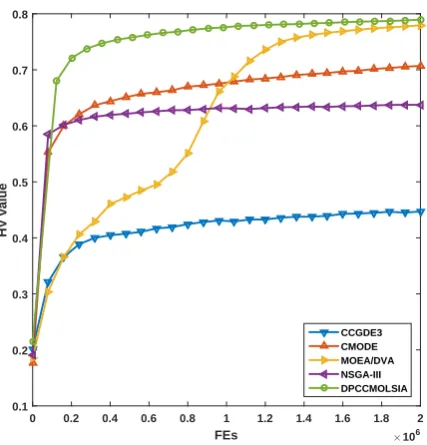
4.4.2. Hilly Terrain

The HV indicator value evolutionary curves for all the algo-rithms for the hilly terrain are illustrated in Fig. 6.

The HV indicator values again reveal that the DPCC-MOLSIA has the best performance (0.7894622), followed by the MOEA/DVA (0.7794569), the CMODE (0.7070007), the NSGA-III (0.6374458), and the CCGDE3 (0.4470647). The characteristics of all the algorithms resemble those described above for the plain terrain.

FEs ×106

0 0.2 0.4 0.6 0.8 1 1.2 1.4 1.6 1.8 2

HV value

0.1 0.2 0.3 0.4 0.5 0.6 0.7 0.8

[image:9.595.362.499.87.763.2]

Figure 6: Evolutionary curves of HV indicator values (hilly ter-rain).

The visualization of the solutions are shown in Fig. 7. Gener-ally, the DPCCMOLSIA more comprehensively approximates the optimal PF and still guarantees good Coverage. As men-tioned above, because the fluctuations in the hilly terrain are relatively smaller and the flat area is larger compared to the mountainous terrain, the algorithms obtain a relatively good

Deployment Cost.

Overall, the performances of the algorithms for the hilly ter-rain can be ordered as follows: DPCCMOLSIA>MOEA/DVA >CMODE>NSGA-III>CCGDE3.

0

0.05

Uniformity 0.1

0.15 0.8 0.6 Coverage

0.4 0.2 0 0.2 0.3 0.4

0 0.1

Cost

(a)

Coverage

0 0.1 0.2 0.3 0.4 0.5 0.6 0.7 0.8

Uniformity

0 0.02 0.04 0.06 0.08 0.1 0.12 0.14

(b)

Cost

0 0.05 0.1 0.15 0.2 0.25 0.3 0.35

Coverage

0 0.1 0.2 0.3 0.4 0.5 0.6 0.7 0.8

(c)

Cost

0 0.05 0.1 0.15 0.2 0.25 0.3 0.35

Uniformity

0 0.02 0.04 0.06 0.08 0.1 0.12 0.14

(d)

[image:9.595.54.268.368.591.2]

(10)

FEs ×106

0 0.2 0.4 0.6 0.8 1 1.2 1.4 1.6 1.8 2

HV value

0.1 0.2 0.3 0.4 0.5 0.6 0.7

[image:10.595.362.499.84.766.2]

Figure 8: Evolutionary curves of HV indicator values (moun-tainous terrain).

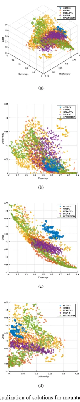
4.4.3. Mountainous Terrain

The HV indicator value evolutionary curves of the DPCC-MOLSIA, the MOEA/DVA, the CMODE, the NSGA-III and the CCGDE3 for the mountainous terrain are illustrated in Fig. 8.

The DPCCMOLSIA again yields the highest HV indicator value (0.6119342), followed by the MOEA/DVA (0.5773018), the CMODE (0.5459146), the NSGA-III (0.4343607), and the CCGDE3 (0.2848895). The characteristics of the different al-gorithms are similar to those for the plain and hilly terrains.

Visualizations of the nondominated solution sets produced by all the algorithms are illustrated in Fig. 9. Overall, the DPC-CMOLSIA performs the best. Because the mountainous terrain has severe altitude variations, it is much more difficult for the algorithms to achieve a good optimization performance.

The performances of all five algorithms for the mountain-ous terrain can be ordered as follows: DPCCMOLSIA > MOEA/DVA>CMODE>NSGA-III>CCGDE3.

Overall, comprehensively considering all the tested terrains, the DPCCMOLSIA is the best in terms of the optimization re-sults; the MOEA/DVA is inferior; the CMODE is the third; the NSGA-III is fourth; and the CCGDE3 is last.

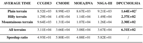
Table 1 summarizes the computation times required by the various algorithms. Compared to the serial algorithms, the computation time of the DPCCMOLSIA is substantially re-duced.

5. Conclusions and Prospects

In the present paper, we put forward a distributed parallel cooperative coevolutionary multi-objective large-scale immune algorithm (DPCCMOLSIA), which uses a three-layer parallel

0 0.05

Uniformity 0.1 0.15 0.2 0.25 1 0.8 Coverage

0.6 0.4 0.2 0 0.6

0.1 0.2 0.3 0.4 0.5

Cost

(a)

Coverage

0.1 0.2 0.3 0.4 0.5 0.6 0.7 0.8 0.9

Uniformity

0 0.05 0.1 0.15 0.2 0.25

(b)

Cost

0.1 0.15 0.2 0.25 0.3 0.35 0.4 0.45 0.5 0.55

Coverage

0.1 0.2 0.3 0.4 0.5 0.6 0.7 0.8 0.9

(c)

Cost

0.1 0.15 0.2 0.25 0.3 0.35 0.4 0.45 0.5 0.55

Uniformity

0 0.05 0.1 0.15 0.2 0.25

(d)

[image:10.595.53.268.92.316.2]

(11)

[image:11.595.40.288.132.208.2]

Table 1: Average Computation Time of the CCGDE3, CMODE, MOEA/DVA, NSGA-III and DPCCMOLSIA, and the Speedup Ratios with Respect to the DPCCMOLSIA

AVERAGE TIME CCGDE3 CMODE MOEA/DVA NSGA-III DPCCMOLSIA

Plain terrain 8.52E+03 8.99E+03 8.67E+03 9.21E+03 1.64E+021 Hilly terrain 1.29E+04 1.45E+04 1.14E+04 1.49E+04 2.37E+02 Mountainous terrain 9.64E+03 1.31E+04 1.07E+04 1.26E+04 2.30E+02

All terrains 3.11E+04 3.66E+04 3.08E+04 3.67E+04 6.31E+02

Speedup ratio 4.93E+01 5.80E+01 4.88E+01 5.82E+01 /

1_{Values in bold denote better performance.}

structure to substantially reduce the computation time. By de-composing the objectives and variables, the original complex MOLSOP is transformed into simpler, small-scale problems that are easier to address. Via tests on real-world terrain data, compared with several other algorithms (CCGDE3, CMODE, MOEA/DVA and NSGA-III), the DPCCMOLSIA can achieve better optimization results in much less time. In the future, we plan to continue improving the DPCCMOLSIA and to test it on additional real-world problems.

Acknowledgments

This work was supported in part by the National Natural Sci-ence Foundation of China (NSFC) under Grant No. 61303001, in part by the Foundation of Key Laboratory of Machine In-telligence and Advanced Computing of the Ministry of Edu-cation under Grant No. MSC-201602A, in part by the Open-ing Project of Guangdong High Performance ComputOpen-ing Soci-ety under Grant No. 2017060101, and in part by the Special Program for Applied Research on Super Computation of the NSFC-Guangdong Joint Fund (the second phase) under Grant No. U1501501. This work was conducted at the National Su-percomputer Center in Guangzhou (NSCC-GZ) and National Supercomputer Center in Tianjin (NSCC-TJ), and the calcula-tions were performed on TianHe-2 and TianHe-1(A). The staff

from the supercomputer centers and the engineers from Beijing Paratera Technology Co., Ltd., provided effective support and made the computation process smooth. Thanks for all the sup-port.

References

[1] B. Cao, J. Zhao, Z. Lv, X. Liu, 3D terrain multiobjective deployment op-timization of heterogeneous directional sensor networks in security mon-itoring, Vol. PP, 2017, pp. 1–1.doi:10.1109/TBDATA.2017.2685581. [2] S. A. Kauffman, Origins of Order in Evolution: Self-Organization and Selection, Springer Netherlands, Dordrecht, 1992, pp. 153–181. doi: 10.1007/978-94-015-8054-0_8.

URLhttp://dx.doi.org/10.1007/978-94-015-8054-0_8

[3] B. Wang, X. Gu, L. Ma, S. Yan, Temperature error correction based on BP neural network in meteorological wireless sensor network, International Journal of Sensor Networks (IJSNET) 23 (4) (2017) 265 – 278. doi: 10.1504/IJSNET.2017.083532.

[4] J. Shen, S. Chang, J. Shen, Q. Liu, X. Sun, A lightweight multi-layer au-thentication protocol for wireless body area networks, Future Generation Computer Systemsdoi:http://dx.doi.org/10.1016/j.future.

2016.11.033.

URL http://www.sciencedirect.com/science/article/pii/

S0167739X16306963

[5] Y. Zhang, X. Sun, B. Wang, Efficient algorithm for k-barrier coverage based on integer linear programming, China Communications 13 (7) (2016) 16–23.doi:10.1109/CC.2016.7559071.

[6] Z. Zhou, Q. J. Wu, F. Huang, X. Sun, Fast and accurate near-duplicate image elimination for visual sensor networks, International Journal of Distributed Sensor Networks 13 (2) (2017) 1550147717694172.arXiv: http://dx.doi.org/10.1177/1550147717694172,doi:10.1177/ 1550147717694172.

URLhttp://dx.doi.org/10.1177/1550147717694172

[7] J. Zhang, J. Tang, T. Wang, F. Chen, Energy-efficient data-gathering ren-dezvous algorithms with mobile sinks for wireless sensor networks, Inter-national Journal of Sensor Networks (IJSNET) 23 (4) (2017) 248 – 257.

doi:10.1504/IJSNET.2017.10004216.

[8] L. N. de Castro, F. J. V. Zuben, Learning and optimization using the clonal selection principle, IEEE Transactions on Evolutionary Compu-tation 6 (3) (2002) 239–251.doi:10.1109/TEVC.2002.1011539. [9] C. A. C. Coello, N. C. Cort´es, An approach to solve multiobjective

opti-mization problems based on an artificial immune system, in: International Conference on Artificial Immune Systems, 2002, pp. 212–221. [10] Y. Xue, J. Jiang, B. Zhao, T. Ma, A self-adaptive artificial bee colony

al-gorithm based on global best for global optimization, Soft Computing (8) (2017) 1–18.doi:10.1007/s00500-017-2547-1.

URLhttps://doi.org/10.1007/s00500-017-2547-1

[11] E. Zitzler, M. Laumanns, L. Thiele, SPEA2: Improving the strength Pareto evolutionary algorithm, Tech. rep., Eidgenössische Technische Hochschule Zürich (ETH), Institut für Technische Informatik und Kom-munikationsnetze (TIK) (2001).doi:10.3929/ethz-a-004284029. [12] K. Deb, A. Pratap, S. Agarwal, T. Meyarivan, A fast and elitist

multiob-jective genetic algorithm: NSGA-II, IEEE Transactions on Evolutionary Computation 6 (2) (2002) 182–197.doi:10.1109/4235.996017. [13] Q. Zhang, H. Li, MOEA/D: A multiobjective evolutionary algorithm

based on decomposition, IEEE Transactions on Evolutionary Computa-tion 11 (6) (2007) 712–731.doi:10.1109/TEVC.2007.892759. [14] T. Zhu, W. Luo, C. Bu, L. Yue, Accelerate population-based stochastic

search algorithms with memory for optima tracking on dynamic power systems, IEEE Transactions on Power Systems 31 (1) (2016) 268–277.

doi:10.1109/TPWRS.2015.2407899.

[15] C. Bu, W. Luo, L. Yue, Continuous dynamic constrained optimization with ensemble of locating and tracking feasible regions strategies, IEEE Transactions on Evolutionary Computation 21 (1) (2017) 14–33. doi: 10.1109/TEVC.2016.2567644.

[16] C. Bu, W. Luo, T. Zhu, L. Yue, Solving online dynamic time-linkage problems under unreliable prediction, Applied Soft Computing 56 (2017) 702 – 716. doi:http://dx.doi.org/10.1016/j.asoc.2016.11. 005.

S1568494616305749

[17] Y. Zhang, W. Luo, Z. Zhang, B. Li, X. Wang, A hard-ware/software partitioning algorithm based on artificial immune principles, Applied Soft Computing 8 (1) (2008) 383 – 391.

doi:http://dx.doi.org/10.1016/j.asoc.2007.03.003.

S1568494607000257

[18] W. Luo, J. Sun, C. Bu, H. Liang, Species-based particle swarm optimizer enhanced by memory for dynamic optimization, Ap-plied Soft Computing 47 (2016) 130 – 140. doi:http: //dx.doi.org/10.1016/j.asoc.2016.05.032.

S1568494616302423

[19] J. Yoo, P. Hajela, Immune network simulations in multicriterion de-sign, Structural optimization 18 (2) (1999) 85–94. doi:10.1007/ BF01195983.

URLhttp://dx.doi.org/10.1007/BF01195983

[20] M. Gong, L. Jiao, H. Du, L. Bo, Multiobjective immune algorithm with nondominated neighbor-based selection, Evolutionary Computation 16 (2) (2008) 225–255.doi:10.1162/evco.2008.16.2.225. [21] Q. Lin, J. Chen, Z. H. Zhan, W. N. Chen, C. A. C. Coello, Y. Yin, C. M.

(12)

multiobjec-tive optimization problems, IEEE Transactions on Evolutionary Compu-tation 20 (5) (2016) 711–729.doi:10.1109/TEVC.2015.2512930. [22] Y.-J. Gong, W.-N. Chen, Z.-H. Zhan, J. Zhang, Y. Li, Q. Zhang, J.-J. Li,

Distributed evolutionary algorithms and their models, Appl. Soft Comput. 34 (C) (2015) 286–300.doi:10.1016/j.asoc.2015.04.061.

URLhttp://dx.doi.org/10.1016/j.asoc.2015.04.061

[23] B. Cao, J. Zhao, Z. Lv, X. Liu, A distributed parallel cooperative coevo-lutionary multiobjective evocoevo-lutionary algorithm for large-scale optimiza-tion, IEEE Transactions on Industrial Informatics 13 (4) (2017) 2030– 2038.doi:10.1109/TII.2017.2676000.

[24] Z. H. Zhan, X. F. Liu, H. Zhang, Z. Yu, J. Weng, Y. Li, T. Gu, J. Zhang, Cloudde: A heterogeneous differential evolution algorithm and its dis-tributed cloud version, IEEE Transactions on Parallel and Disdis-tributed Sys-tems 28 (3) (2017) 704–716.doi:10.1109/TPDS.2016.2597826. [25] D. A. V. Veldhuizen, J. B. Zydallis, G. B. Lamont, Considerations in

en-gineering parallel multiobjective evolutionary algorithms, IEEE Trans-actions on Evolutionary Computation 7 (2) (2003) 144–173. doi:10. 1109/TEVC.2003.810751.

[26] A. J. Nebro, J. J. Durillo, A Study of the Parallelization of the Multi-Objective Metaheuristic MOEA/D, Springer Berlin Heidelberg, Berlin, Heidelberg, 2010, pp. 303–317.doi:10.1007/978-3-642-13800-3_ 32.

[27] J. J. Durillo, Q. Zhang, A. J. Nebro, E. Alba, Distribution of Compu-tational Effort in Parallel MOEA/D, Springer Berlin Heidelberg, Berlin, Heidelberg, 2011, pp. 488–502.doi:10.1007/978-3-642-25566-3_ 38.

[28] J. Ge, Z. Chen, Y. Wu, Y. E, H-SOFT: a heuristic storage space opti-misation algorithm for flow table of openflow, Concurrency and Com-putation: Practice and Experience 27 (13) (2015) 3497–3509, cPE-13-0288.R1.doi:10.1002/cpe.3206.

URLhttp://dx.doi.org/10.1002/cpe.3206

[29] B. Cao, J. Zhao, Z. Lv, X. Liu, S. Yang, X. Kang, K. Kang, Dis-tributed parallel particle swarm optimization for multi-objective and many-objective large-scale optimization, IEEE Access 5 (2017) 8214– 8221.doi:10.1109/ACCESS.2017.2702561.

[30] X. Ma, F. Liu, Y. Qi, X. Wang, L. Li, L. Jiao, M. Yin, M. Gong, A multiobjective evolutionary algorithm based on decision variable anal-yses for multiobjective optimization problems with large-scale variables, IEEE Transactions on Evolutionary Computation 20 (2) (2016) 275–298.

doi:10.1109/TEVC.2015.2455812.

[31] J. J. Escobar, J. Ortega, J. Gonz´alez, M. Damas, Assessing Parallel Het-erogeneous Computer Architectures for Multiobjective Feature Selection on EEG Classification, Springer International Publishing, Cham, 2016, pp. 277–289.doi:10.1007/978-3-319-31744-1_25.

[32] A. G. D. Nuovo, M. Palesi, V. Catania, Multi-objective evolutionary fuzzy clustering for high-dimensional problems, in: 2007 IEEE Interna-tional Fuzzy Systems Conference, 2007, pp. 1–6.doi:10.1109/FUZZY. 2007.4295660.

[33] Y. Zuo, M. Gong, J. Zeng, L. Ma, L. Jiao, Personalized recommenda-tion based on evolurecommenda-tionary multi-objective optimizarecommenda-tion [research fron-tier], IEEE Computational Intelligence Magazine 10 (1) (2015) 52–62.

doi:10.1109/MCI.2014.2369894.

[34] M. A. Potter, K. A. De Jong, A cooperative coevolutionary approach to function optimization, Springer Berlin Heidelberg, Berlin, Heidelberg, 1994, pp. 249–257.doi:10.1007/3-540-58484-6_269.

URLhttp://dx.doi.org/10.1007/3-540-58484-6_269

[35] F. van den Bergh, A. P. Engelbrecht, A cooperative approach to particle swarm optimization 8 (3) (2004) 225–239.doi:10.1109/TEVC.2004. 826069.

[36] M. N. Omidvar, X. Li, X. Yao, Cooperative co-evolution with delta grouping for large-scale non-separable function optimization, in: Proc. IEEE Congr. Evol. Comput., 2010, pp. 1–8.doi:10.1109/CEC.2010. 5585979.

[37] X. Li, X. Yao, Cooperatively coevolving particle swarms for large-scale optimization, IEEE Trans. Evol. Comput. 16 (2) (2012) 210–224. doi: 10.1109/TEVC.2011.2112662.

[38] M. N. Omidvar, X. Li, Y. Mei, X. Yao, Cooperative co-evolution with dif-ferential grouping for large-scale optimization, IEEE Trans. Evol.

Com-put. 18 (3) (2014) 378–393.doi:10.1109/TEVC.2013.2281543. [39] Y. Mei, M. N. Omidvar, X. Li, X. Yao, A competitive divide-and-conquer

algorithm for unconstrained large-scale black-box optimization, ACM Trans. Math. Softw. 42 (2) (2016) 13:1–13:24.doi:10.1145/2791291.

URLhttp://doi.acm.org/10.1145/2791291

[40] Y. Ling, H. Li, B. Cao, Cooperative co-evolution with graph-based diff er-ential grouping for large scale global optimization, in: 2016 12th Interna-tional Conference on Natural Computation, Fuzzy Systems and Knowl-edge Discovery (ICNC-FSKD), 2016, pp. 95–102.doi:10.1109/FSKD. 2016.7603157.

[41] L. M. Antonio, C. A. C. Coello, Use of cooperative coevolution for solv-ing large scale multiobjective optimization problems, in: 2013 IEEE Congress on Evolutionary Computation, 2013, pp. 2758–2765. doi: 10.1109/CEC.2013.6557903.

[42] S. Huband, P. Hingston, L. Barone, L. While, A review of multiobjec-tive test problems and a scalable test problem toolkit, IEEE Trans. Evol. Comput. 10 (5) (2006) 477–506.doi:10.1109/TEVC.2005.861417. [43] J. Wang, W. Zhang, J. Zhang, Cooperative differential evolution with

multiple populations for multiobjective optimization, IEEE Transactions on Cybernetics 46 (12) (2016) 2848–2861.doi:10.1109/TCYB.2015. 2490669.

[44] Y. Wu, G. Min, K. Li, B. Javadi, Modeling and analysis of communica-tion networks in multicluster systems under spatio-temporal bursty traf-fic, IEEE Transactions on Parallel and Distributed Systems 23 (5) (2012) 902–912.doi:10.1109/TPDS.2011.198.

[45] Y. Wu, G. Min, D. Zhu, L. T. Yang, An analytical model for on-chip inter-connects in multimedia embedded systems, ACM Trans. Embed. Comput. Syst. 13 (1s) (2013) 29:1–29:19.doi:10.1145/2536747.2536751.

URLhttp://doi.acm.org/10.1145/2536747.2536751

[46] K. Deb, H. Jain, An evolutionary many-objective optimization algorithm using reference-point-based nondominated sorting approach, part I: Solv-ing problems with box constraints, IEEE Transactions on Evolution-ary Computation 18 (4) (2014) 577–601. doi:10.1109/TEVC.2013. 2281535.

[47] E. Zitzler, L. Thiele, M. Laumanns, C. M. Fonseca, V. G. da Fonseca, Performance assessment of multiobjective optimizers: An analysis and review, IEEE Transactions on Evolutionary Computation 7 (2) (2003) 117–132.doi:10.1109/TEVC.2003.810758.