Using EMD-FrFT filtering to mitigate high power interference in chirp tracking radars

(1)

IEEE Proof

Web Version

Abstract—This letter presents a new signal processing

sub-system for conventional monopulse tracking radars that offers an improved solution to the problem of dealing with manmade high power interference (jamming). It is based on the hybrid use of empirical mode decomposition (EMD) and fractional Fourier transform (FrFT). EMD-FrFTfiltering is carried out for complex noisy radar chirp signals to decrease the signal’s noisy compo-nents. An improvement in the signal-to-noise ratio (SNR) of up to 18 dB for different target SNRs is achieved using the proposed EMD-FrFT algorithm.

Index Terms—Empirical mode decomposition, fractional Fourier transforms, high power interference suppression.

I. INTRODUCTION

A

high power noise interference introduced to a monopulse tracking radar processor through the radar antenna pro-duces an interference error that affects the radar tracking ability and may cause target mistracking [1]. Various methods [2]–[4] for combating high noise power interference have been pub-lished.

In our previous work [1] the mistracking problem due to in-terference signals was addressed using thefiltering in the Frac-tional Fourier Transform domain. In this letter we propose the use of both empirical mode decomposition (EMD) and frac-tional Fourier transform (FrFT) to implement EMD-FrFTfi l-ters in an attempt to reduce the very high power interference sig-nals introduced from the antenna main lobe or from the antenna side lobes for radar receiving channels. Following a brief in-troduction on EMD and FrFT the letter then describes the struc-ture of the new EMD-FrFTfiltering algorithm based monopulse radar processor. The superior performance of the new algorithm is demonstrated using a set of simulation results.

II. CLASSICAL ANDBIVARIATEEMD

The intrinsic mode functions (IMFs) of an EMD signal de-composition are oscillatory and have no DC component, so the signal in the EMD domain may be represented as [5]

(1)

Manuscript received November 30, 2010; revised January 27, 2011; accepted February 07, 2011. The associate editor coordinating the review of this manu-script and approving it for publication was Prof. Amir Asif.

The authors are with The Centre for Excellence in Signal and Image Processing, Department of Electronic and Electrical Engineering, University of Strathclyde, Glasgow, U.K. (e-mail: [email protected]; [email protected]).

Color versions of one or more of thefigures in this paper are available online at http://ieeexplore.ieee.org.

Digital Object Identifier 10.1109/LSP.2011.2115239

where , are the IMFs and is the

residual. When a signal , comprising a slow oscillation su-perimposed on a highly oscillating signal (in our case additive high power interference noise signal), is applied to an EMD al-gorithm, thefirst few IMFs tend to contain the highly oscillation signal (noise) and the remaining IMFs contain the useful signal (in our case radar chirp signal).

The bivariate EMD [6] may be used for complex valued time series. As with the classical EMD, the bivariate EMD is used to separate the more rapidly rotating components from slower ones. The procedure is to define the slowly rotating compo-nent as the mean of some envelope which is a three-dimensional cylinder that encloses the signal. In our work the bivariate EMD (complex EMD) is used to decompose the complex radar signal into a complete andfinite set of complex IMFs in order to sub-sequently minimise the additive noise interference.

The concept of detrending in high frequency noise environ-ments is to calculate an estimate of the IMF number at which all previous IMFs may be regarded as noise and the subsequent IMFs may be considered to contain the useful signal compo-nents.

The IMF detrending technique assumes that the 1st IMF, , captures mostly noise, the noise level is estimated in by computing [5]

(2)

where is the number of samples. The model for noise only IMF energies can be approximated for white Gaussian noise dependence on the energy of thefirst IMF from [5]

(3)

The threshold level energies are used to distinguish be-tween signal and noise. They are calculated using the approxi-mated IMF energies in (3) from [5]

(4)

Computing the IMFs energies by applying the EMD algo-rithm on (noisy signal) from [5]

(5)

Comparing IMFs energies with the threshold level ener-gies allows us to determine exactly when the signal energy level crosses the threshold level.

Assuming this occurs at , the signal is denoised by reconstruction using only IMFs whose energy exceeds the threshold according to:

(2)

IEEE Proof

Web Version

2 IEEE SIGNAL PROCESSING LETTERS, VOL. 18, NO. 4, APRIL 2011

Fig. 1. Detrending and the thresholding.

(6)

In Fig. 1 the EMD algorithm is applied to a noisy signal re-sulting in 10 IMFs. Using (2) and (3) the 1st IMF is used to estimate the noise only energies for the remaining IMFs. The resulting noise only model outputs are shown in Fig. 1. The ac-tual IMFs energies calculated from (5) are also illustrated on Fig. 1 along with the threshold model for each IMF. It is clear that the actual IMFs energies are close to those estimated for the noise only model up to IMF 6 at which the threshold level is crossed. This means that these IMFs (from 1 to 6) may be re-garded as essentially noise only. Thus, the sum of IMFs from 7 to 10 represents the detrended and thresholded signal.

For the noisy signal, a higher sampling frequency yields a higher number of samples and as a result a greater number of IMFs using the EMD algorithm. Consequently a higher accu-racy of detrending IMFs in the EMD-DT algorithm is expected. This concept of detrending and thresholding is used later in Section V.

III. FRACTIONALFOURIERTRANSFORM

The fractional Fourier transform of order of an arbitrary function , with an angle is defined as [7], [8]

(7)

where is the transformation kernel, is the

transfor-mation of to the order, and with . The

optimum order value, for a chirp signal may be computed as [9]

(8)

where is the sampling frequency, is the chirp duration, is the number of samples in the time received window, and is the chirp bandwidth.

Fig. 2. Basic structure of monopulse radar.

IV. MONOPULSERADARSIGNAL

A block diagram of a typical monopulse radar is shown in Fig. 2. A pulsed chirp signal is produced from the waveform generator. This is up-converted to the radar carrier frequency, amplified and passed through the duplexer to be transmitted:

(9)

where is the time, is the chirp start frequency, and is the chirp stop frequency. This is up-converted to the radar carrier frequency, amplified and passed through the duplexer to be transmitted. The down-converted received signal passes through a band limited Gaussian before passing through the chirp matchedfilter to maximize the target return signal. The target information parameters (azimuth angle, elevation angle, and target range) are then calculated by the monopulse processor from thefiltered signal.

The structure of monopulse radar shown in Fig. 2 is repeated times ( equal to the of array antenna elements). Thus each antenna will have its own complete receiving system and all the output data will be processed using only one monopulse pro-cessor.

The radar received chirp signal may be expressed in the baseband as [1] shown in the equation at bottom of page, where is the received signal amplitude, is a random phase shift,

is the Doppler vector, is antenna phase factor, and is the start time of the returned pulse.

The start time depends on the target range and can be computed from

(11)

where is the speed of light. As indicated in (10) the Doppler shift and delay effect on the target chirp signal is determined

(3)

IEEE Proof

Web Version

by the dot product of the chirp signal by the Doppler vector defined as

(12) where is the target Doppler frequency.

For the phased array receiving antenna, an antenna phase factor is introduced as

(13)

where is a vector represented as ,

is a unitary vector, and is calculated from

(14) where is the separation between the antenna elements, is the target angle from the antenna boresight.

V. FILTERINGBASEDEMD-FRFT ALGORITHM It is proposed to combat the high power noise interference byfiltering the received signal in the optimal fractional Fourier transform (FrFT) domain using the transmitted chirp radar infor-mation. Normally the magnitude of chirp signal in the optimum FrFT domain would be significantly higher than the noise signal in the fractional domain [1]. However in high power jamming scenarios this is not usually true and it becomes difficult to dis-tinguish between the target spike and the noise spikes in the op-timal FrFT domain.

The proposed EMD-FrFT radarfiltering process, which must be applied to the received signal before the band passfilter, is shown in Fig. 3. The radar received noisy complex chirp signal is sampled using the radar sampling frequency to form . The signal recovery is carried out in two stages: i) EMD Filtering Stage and ii) the FrFT Filtering Stage.

EMD Filtering Stage: In stage one the received signal is input to a bivariate EMD to produce the complex IMFs . The complex IMFs are detrended and thresholded to estimate the non-noisy IMFs using (2)–(5) as described in Section II. Only IMFs whose energy exceeds the threshold are retained. The resultant thresholded IMFs are combined to produce the complex denoised signal as in (6).

FrFT Filtering Stage [1]: For the second stage, the com-plex denoised signal in the optimal fractional domain is calcu-lated from the information supplied from the transmitted chirp signal as in (8). Knowing the peak position of the target chirp signal in the optimum FrFT domain, the received data isfiltered by keeping the chirp target data (peak position sample and its adjacent samples) and forces all the remaining samples in the tracking window to zero. The inverse FrFT is used with the known optimal order to transform the signal back to time do-main afterfiltering. The EMD-FrFTfiltered data is supplied to the radar processor to continue data processing to calculate the target information.

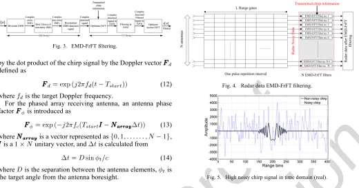
The EMD-FrFTfiltering process illustrated in Fig. 3 is at-tached to receiving channels in which the received signal from each of the antenna elements willfill range gates.

Fig. 4. Radar data EMD-FrFTfiltering.

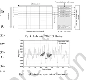
Fig. 5. High noisy chirp signal in time domain (real).

The total radar data size is therefore equal to for each pulse return. The EMD-FrFTfilter block seen in Fig. 4 consists of EMD-FrFTfilters shown in Fig. 3. The overallfiltered data are processed to determine the target information pa-rameters as illustrated in Fig. 2.

VI. SIMULATIONRESULTS

The computer based simulations comprise an array of 14 elements spaced 1/3 m apart. The radar pulse width is 100 microseconds and a pulse repetition interval of 1.6 ms for a 435 MHz carrier was used. The incoming baseband signals are sampled at 1 MHz. Also it is assumed that the radar operating range is 100:200 range bins with a starting window at 865 m and a window duration of 403 m. The target is considered at at angle 32 from the look direction with target signal to noise ratio (SNR) set to 56 dB. A jamming signal with interference noise ratio (INR) set to 75 dB at angle 32 from the look direction (main beam jamming) is introduced.1

A. High Power Interference Scenario

Considering the simulation parameters for one of the 14 re-ceiving channels (first channel), the receiving target chirp signal appears at range bin 150 in case of no jamming while the chirp signal is completely corrupted in the time domain (also in the frequency domain) by the noise due to high power jamming signal as seen in Fig. 5.

The bivariate EMD is applied to the noisy signal to produce the complex IMFs. A sampling frequency is increased to 10 MHz (ten times the radar sampling frequency ) to increase the number of IMFs.

The resultant complex IMFs from applying the bivariate EMD to the noisy chirp 1 4029 produces 14 IMFs each of length 4029. Keeping only IMFs whose energy exceeds the threshold using the EMD-DT algorithm described in Section II the signal is reconstructed summing the non-noisy IMFs from

1_{The simulations parameters are extracted from DARPA/Navy Mountaintop}

[image:3.592.41.561.61.334.2]

(4)

IEEE Proof

Web Version

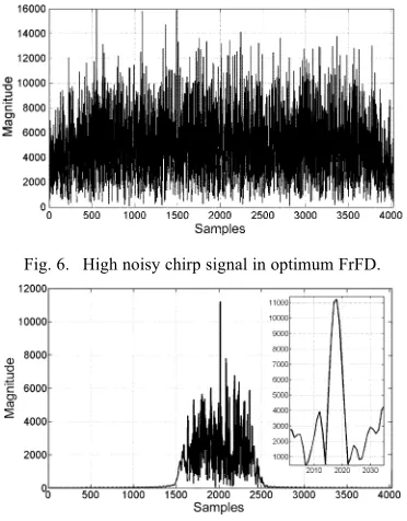
Fig. 6. High noisy chirp signal in optimum FrFD.

Fig. 7. EMD denoised chirp in optimum FrFD.

6 to 14 to obtain the filtered signal after applying EMD-DT algorithm.

Substituting the monopulse radar parameter values given above into (8) with a high sampling frequency of 10 MHz, the order of the optimal FrFT domain is computed as 1.1266. The EMD filtered signal is transferred to the optimal FrFD using the optimal order FrFT domain 1.1266.

Transforming the radar received signal directly to the op-timum FrFD using the calculated , is expected to produce a high magnitude value (spike) due to transferring the chirp signal to the optimum FrFD. However as seen in Fig. 6 due to the high power interference the spike of the target chirp is highly cor-rupted also by noise spikes in the optimum FrFD and cannot be

filtered in this domain.

It is therefore difficult to distinguish between the target spike and the noise spikes in the optimal FrFD. The proposed EMD-FrFTfiltering algorithm is used to address this problem. Fig. 7 shows the EMD denoised chirp in optimum FrFD. It is evident that the noise is significantly reduced especially the high fre-quency components and the chirp target spike is also the highest spike which is shown in the zoomed portion of Fig. 7.

The proposedfiltering algorithm in the optimum FrFD keeps the sample with maximum magnitude (sample no. 2018) and its ten adjacent samples from 2013–2023 while forcing all other samples window to zero. Thefiltered signal is then transformed back to time domain by applying inverse optimum FrFT using— ( 1.1266) by applying (7). The real and imagi-nary parts of the denoised signal (recovered) after applying the proposed EMD-FrFTfiltering algorithm is shown in Fig. 3.

Fig. 8 compares the denoised chirp signal using EMD-FrFT

filter with the non noisy signal. In the simulation example, the considered signal total input SNR is approximately equal 8 dB (after adding the jamming noise) and the output SNR is approx-imately 10 dB. The proposed EMD-FrFTfiltering algorithm of-fers signal enhancement of approximately 18 dB.

[image:4.592.73.259.62.300.2]

B. Signal Improvement at Different SNR

[image:4.592.304.556.63.140.2]

Table I shows the improvement results of applying different target SNR for the same jamming scenario (INR set to 75 dB

Fig. 8. Recovered chirp signal. (a) Real; (b) imaginary.

TABLE I

THEIMPROVEMENTRESULTS INdBFORMONOPULSEPROCESSORS

at angle 32 ) and calculating the total input SNRs to the radar receiving channel. The results in Table I comprise an average over 50 independent noise generations.

Table I indicates an improvement of approximately 18.1 dBs

for input and an improvement of

approxi-mately 4.9 dBs for input . The proposed EMD-FrFT algorithm yields a higher improvement for the lower SNRs rather than the higher SNRs.

VII. CONCLUSION

A system to reduce the distortion problem due to high power interference in chirp radar systems is presented. The proposed EMD-FrFTfiltering algorithm successfully decreases the high power noise interference and improves the received radar SNR. A resulting improvement in the radar received signal is obtained for different SNR and the highest gain is achieved in the case of lower SNR (up to 18 dB in the considered case).

REFERENCES

[1] S. A. Elgamel and J. J. Soraghan, “Enhanced monopulse radar tracking using fractional fourierfiltering in the presence of interference,” in11th Int. Radar Symp. (IRS), 2010 11th International, 2010, pp. 1–4. [2] A. Farina, G. Golino, and L. Timmoneri, “Maximum likelihood

esti-mator approach to determine the target angular co-ordinates in pres-ence of main beam interferpres-ence: Application to live data acquired with a microwave phased array radar,” inIEEE Int. Radar Conf., 2005, pp. 61–66.

[3] Y. Seliktar, E. J. Holder, and D. B. Williams, A Space/Fast-Time Adap-tive Monopulse Technique. New York: Hindawi, 2006, pp. 218–228. [4] J. Zongsheng and S. Xicai, “Analysis on the tracking performance of active radar seeker under the condition of coherent interference,” in

IEEE Int. Conf. Intelligent Computing and Intelligent Systems, 2009, pp. 418–422.

[5] P. Flandrin, P. Goncalves, and G. Rilling, “Detrending and denoising with empirical mode decompositions,” in2004 Eur. Signal Processing Conf. (EUSIPCO-2004), 2004.

[6] G. Rilling, P. Flandrin, P. Gonalves, and J. M. Lilly, “Bivariate em-pirical mode decomposition,”IEEE Signal Process. Lett., vol. 14, pp. 936–939, 2007.

[7] C. Candan, M. A. Kutay, and H. M. Ozaktas, “The discrete frac-tional fourier transform,”IEEE Trans. Signal Process., vol. 48, pp. 1329–1337, 2000.

[8] H. M. Ozaktas, G. Zalevsky, and M. A. Kutay, The Fractional Fourier Transform: With Applications in Optics and Signal Processing. New York: Wiley, Jan. 2001.

(5)

IEEE Proof

Print Version

Abstract—This letter presents a new signal processing

sub-system for conventional monopulse tracking radars that offers an improved solution to the problem of dealing with manmade high power interference (jamming). It is based on the hybrid use of empirical mode decomposition (EMD) and fractional Fourier transform (FrFT). EMD-FrFTfiltering is carried out for complex noisy radar chirp signals to decrease the signal’s noisy compo-nents. An improvement in the signal-to-noise ratio (SNR) of up to 18 dB for different target SNRs is achieved using the proposed EMD-FrFT algorithm.

Index Terms—Empirical mode decomposition, fractional Fourier transforms, high power interference suppression.

I. INTRODUCTION

A

high power noise interference introduced to a monopulse

tracking radar processor through the radar antenna pro-duces an interference error that affects the radar tracking ability and may cause target mistracking [1]. Various methods [2]–[4] for combating high noise power interference have been pub-lished.

In our previous work [1] the mistracking problem due to

in-terference signals was addressed using thefiltering in the

Frac-tional Fourier Transform domain. In this letter we propose the use of both empirical mode decomposition (EMD) and

frac-tional Fourier transform (FrFT) to implement EMD-FrFTfi

l-ters in an attempt to reduce the very high power interference sig-nals introduced from the antenna main lobe or from the antenna

side lobes for radar receiving channels. Following a brief

in-troduction on EMD and FrFT the letter then describes the

struc-ture of the new EMD-FrFTfiltering algorithm based monopulse

radar processor. The superior performance of the new algorithm is demonstrated using a set of simulation results.

II. CLASSICAL ANDBIVARIATEEMD

The intrinsic mode functions (IMFs) of an EMD signal de-composition are oscillatory and have no DC component, so the

signal in the EMD domain may be represented as [5]

(1)

Manuscript received November 30, 2010; revised January 27, 2011; accepted February 07, 2011. The associate editor coordinating the review of this manu-script and approving it for publication was Prof. Amir Asif.

The authors are with The Centre for Excellence in Signal and Image Processing, Department of Electronic and Electrical Engineering, University of Strathclyde, Glasgow, U.K. (e-mail: [email protected]; [email protected]).

Color versions of one or more of thefigures in this paper are available online at http://ieeexplore.ieee.org.

Digital Object Identifier 10.1109/LSP.2011.2115239

where , are the IMFs and is the

residual. When a signal , comprising a slow oscillation

su-perimposed on a highly oscillating signal (in our case additive high power interference noise signal), is applied to an EMD

al-gorithm, thefirst few IMFs tend to contain the highly oscillation

signal (noise) and the remaining IMFs contain the useful signal (in our case radar chirp signal).

The bivariate EMD [6] may be used for complex valued time series. As with the classical EMD, the bivariate EMD is used to separate the more rapidly rotating components from slower

ones. The procedure is to define the slowly rotating

compo-nent as the mean of some envelope which is a three-dimensional cylinder that encloses the signal. In our work the bivariate EMD (complex EMD) is used to decompose the complex radar signal

into a complete andfinite set of complex IMFs in order to

sub-sequently minimise the additive noise interference.

The concept of detrending in high frequency noise environ-ments is to calculate an estimate of the IMF number at which all previous IMFs may be regarded as noise and the subsequent IMFs may be considered to contain the useful signal compo-nents.

The IMF detrending technique assumes that the 1st IMF,

, captures mostly noise, the noise level is estimated

in by computing [5]

(2)

where is the number of samples. The model for noise only

IMF energies can be approximated for white Gaussian noise

dependence on the energy of thefirst IMF from [5]

(3)

The threshold level energies are used to distinguish

be-tween signal and noise. They are calculated using the approxi-mated IMF energies in (3) from [5]

(4)

Computing the IMFs energies by applying the EMD

algo-rithm on (noisy signal) from [5]

(5)

Comparing IMFs energies with the threshold level

ener-gies allows us to determine exactly when the signal energy

level crosses the threshold level.

Assuming this occurs at , the signal is denoised

by reconstruction using only IMFs whose energy exceeds the threshold according to:

(6)

IEEE Proof

Print Version

Fig. 1. Detrending and the thresholding.

(6)

In Fig. 1 the EMD algorithm is applied to a noisy signal re-sulting in 10 IMFs. Using (2) and (3) the 1st IMF is used to estimate the noise only energies for the remaining IMFs. The resulting noise only model outputs are shown in Fig. 1. The ac-tual IMFs energies calculated from (5) are also illustrated on Fig. 1 along with the threshold model for each IMF. It is clear that the actual IMFs energies are close to those estimated for the noise only model up to IMF 6 at which the threshold level is crossed. This means that these IMFs (from 1 to 6) may be re-garded as essentially noise only. Thus, the sum of IMFs from 7 to 10 represents the detrended and thresholded signal.

For the noisy signal, a higher sampling frequency yields a higher number of samples and as a result a greater number of IMFs using the EMD algorithm. Consequently a higher accu-racy of detrending IMFs in the EMD-DT algorithm is expected. This concept of detrending and thresholding is used later in Section V.

III. FRACTIONALFOURIERTRANSFORM

The fractional Fourier transform of order of an arbitrary

function , with an angle is defined as [7], [8]

(7)

where is the transformation kernel, is the

transfor-mation of to the order, and with . The

optimum order value, for a chirp signal may be computed

as [9]

(8)

where is the sampling frequency, is the chirp duration,

is the number of samples in the time received window, and is the chirp bandwidth.

Fig. 2. Basic structure of monopulse radar.

IV. MONOPULSERADARSIGNAL

A block diagram of a typical monopulse radar is shown in

Fig. 2. A pulsed chirp signal is produced from the waveform

generator. This is up-converted to the radar carrier frequency,

amplified and passed through the duplexer to be transmitted:

(9)

where is the time, is the chirp start frequency, and

is the chirp stop frequency. This is up-converted to the radar

carrier frequency, amplified and passed through the duplexer

to be transmitted. The down-converted received signal passes through a band limited Gaussian before passing through the

chirp matchedfilter to maximize the target return signal. The

target information parameters (azimuth angle, elevation angle, and target range) are then calculated by the monopulse processor from thefiltered signal.

The structure of monopulse radar shown in Fig. 2 is repeated

times ( equal to the of array antenna elements). Thus each

antenna will have its own complete receiving system and all the output data will be processed using only one monopulse pro-cessor.

The radar received chirp signal may be expressed in the

baseband as [1] shown in the equation at bottom of page, where

is the received signal amplitude, is a random phase shift,

is the Doppler vector, is antenna phase factor, and

is the start time of the returned pulse.

The start time depends on the target range and can

be computed from

(11)

where is the speed of light. As indicated in (10) the Doppler

shift and delay effect on the target chirp signal is determined

(7)

IEEE Proof

Print Version

by the dot product of the chirp signal by the Doppler vector defined as

(12)

where is the target Doppler frequency.

For the phased array receiving antenna, an antenna phase

factor is introduced as

(13)

where is a vector represented as ,

is a unitary vector, and is calculated from

(14)

where is the separation between the antenna elements, is

the target angle from the antenna boresight.

V. FILTERINGBASEDEMD-FRFT ALGORITHM It is proposed to combat the high power noise interference

byfiltering the received signal in the optimal fractional Fourier

transform (FrFT) domain using the transmitted chirp radar infor-mation. Normally the magnitude of chirp signal in the optimum

FrFT domain would be significantly higher than the noise signal

in the fractional domain [1]. However in high power jamming

scenarios this is not usually true and it becomes difficult to

dis-tinguish between the target spike and the noise spikes in the op-timal FrFT domain.

The proposed EMD-FrFT radarfiltering process, which must

be applied to the received signal before the band passfilter, is

shown in Fig. 3. The radar received noisy complex chirp signal

is sampled using the radar sampling frequency to form .

The signal recovery is carried out in two stages: i) EMD

Filtering Stage and ii) the FrFT Filtering Stage.

EMD Filtering Stage: In stage one the received signal is

input to a bivariate EMD to produce the complex IMFs .

The complex IMFs are detrended and thresholded to estimate the non-noisy IMFs using (2)–(5) as described in Section II. Only IMFs whose energy exceeds the threshold are retained. The resultant thresholded IMFs are combined to produce the complex denoised signal as in (6).

FrFT Filtering Stage [1]: For the second stage, the

com-plex denoised signal in the optimal fractional domain is calcu-lated from the information supplied from the transmitted chirp signal as in (8). Knowing the peak position of the target chirp

signal in the optimum FrFT domain, the received data isfiltered

by keeping the chirp target data (peak position sample and its adjacent samples) and forces all the remaining samples in the tracking window to zero. The inverse FrFT is used with the known optimal order to transform the signal back to time

do-main afterfiltering. The EMD-FrFTfiltered data is supplied to

the radar processor to continue data processing to calculate the target information.

The EMD-FrFT filtering process illustrated in Fig. 3 is

at-tached to receiving channels in which the received signal

from each of the antenna elements willfill range gates.

Fig. 4. Radar data EMD-FrFTfiltering.

Fig. 5. High noisy chirp signal in time domain (real).

The total radar data size is therefore equal to for each

pulse return. The EMD-FrFTfilter block seen in Fig. 4 consists

of EMD-FrFTfilters shown in Fig. 3. The overallfiltered data

are processed to determine the target information pa-rameters as illustrated in Fig. 2.

VI. SIMULATIONRESULTS

The computer based simulations comprise an array of 14 elements spaced 1/3 m apart. The radar pulse width is 100 microseconds and a pulse repetition interval of 1.6 ms for a 435 MHz carrier was used. The incoming baseband signals are sampled at 1 MHz. Also it is assumed that the radar operating range is 100:200 range bins with a starting window at 865 m and a window duration of 403 m. The target is considered at at angle 32 from the look direction with target signal to noise ratio (SNR) set to 56 dB. A jamming signal with interference noise ratio (INR) set to 75 dB at angle 32

from the look direction (main beam jamming) is introduced.1

A. High Power Interference Scenario

Considering the simulation parameters for one of the 14

re-ceiving channels (first channel), the receiving target chirp signal

appears at range bin 150 in case of no jamming while the chirp signal is completely corrupted in the time domain (also in the frequency domain) by the noise due to high power jamming signal as seen in Fig. 5.

The bivariate EMD is applied to the noisy signal to produce the complex IMFs. A sampling frequency is increased to 10

MHz (ten times the radar sampling frequency ) to increase

the number of IMFs.

The resultant complex IMFs from applying the bivariate

EMD to the noisy chirp 1 4029 produces 14 IMFs each of

length 4029. Keeping only IMFs whose energy exceeds the threshold using the EMD-DT algorithm described in Section II the signal is reconstructed summing the non-noisy IMFs from

1_{The simulations parameters are extracted from DARPA/Navy Mountaintop}

[image:7.612.274.575.62.342.2]

(8)

IEEE Proof

Print Version

Fig. 6. High noisy chirp signal in optimum FrFD.

Fig. 7. EMD denoised chirp in optimum FrFD.

6 to 14 to obtain the filtered signal after applying EMD-DT

algorithm.

Substituting the monopulse radar parameter values given above into (8) with a high sampling frequency of 10 MHz, the

order of the optimal FrFT domain is computed as 1.1266.

The EMD filtered signal is transferred to the optimal FrFD

using the optimal order FrFT domain 1.1266.

Transforming the radar received signal directly to the

op-timum FrFD using the calculated , is expected to produce a

high magnitude value (spike) due to transferring the chirp signal to the optimum FrFD. However as seen in Fig. 6 due to the high power interference the spike of the target chirp is highly cor-rupted also by noise spikes in the optimum FrFD and cannot be

filtered in this domain.

It is therefore difficult to distinguish between the target spike and the noise spikes in the optimal FrFD. The proposed

EMD-FrFTfiltering algorithm is used to address this problem. Fig. 7

shows the EMD denoised chirp in optimum FrFD. It is evident

that the noise is significantly reduced especially the high

fre-quency components and the chirp target spike is also the highest spike which is shown in the zoomed portion of Fig. 7.

The proposedfiltering algorithm in the optimum FrFD keeps

the sample with maximum magnitude (sample no. 2018) and its ten adjacent samples from 2013–2023 while forcing all other

samples window to zero. Thefiltered signal is then transformed

back to time domain by applying inverse optimum FrFT

using— ( 1.1266) by applying (7). The real and

imagi-nary parts of the denoised signal (recovered) after applying the

proposed EMD-FrFTfiltering algorithm is shown in Fig. 3.

Fig. 8 compares the denoised chirp signal using EMD-FrFT

filter with the non noisy signal. In the simulation example, the

considered signal total input SNR is approximately equal 8 dB

(after adding the jamming noise) and the output SNR is

approx-imately 10 dB. The proposed EMD-FrFTfiltering algorithm

of-fers signal enhancement of approximately 18 dB.

[image:8.612.74.260.65.308.2]

B. Signal Improvement at Different SNR

[image:8.612.304.555.67.143.2]

Table I shows the improvement results of applying different target SNR for the same jamming scenario (INR set to 75 dB

Fig. 8. Recovered chirp signal. (a) Real; (b) imaginary.

TABLE I

THEIMPROVEMENTRESULTS INdBFORMONOPULSEPROCESSORS

at angle 32 ) and calculating the total input SNRs to the radar receiving channel. The results in Table I comprise an average over 50 independent noise generations.

Table I indicates an improvement of approximately 18.1 dBs

for input and an improvement of

approxi-mately 4.9 dBs for input . The proposed

EMD-FrFT algorithm yields a higher improvement for the lower SNRs rather than the higher SNRs.

VII. CONCLUSION

A system to reduce the distortion problem due to high power interference in chirp radar systems is presented. The proposed

EMD-FrFTfiltering algorithm successfully decreases the high

power noise interference and improves the received radar SNR. A resulting improvement in the radar received signal is obtained for different SNR and the highest gain is achieved in the case of lower SNR (up to 18 dB in the considered case).