Determining the Number of Factors in a Multivariate
Error Correction–Volatility Factor Model
Qiaoling Li† and Jiazhu Pan†‡
†School of Mathematical Sciences, Peking University, Beijing 100871, China Email: [email protected]
‡Department of Statistics and Modelling Science, University of Strathclyde, U.K. Email: [email protected]
Summary In order to describe the comovements in both conditional mean and conditional variance of high dimensional nonstationary time series by dimension reduction, we introduce the conditional heteroscedasticity with factor structure to the error correction model. The new model is called the error correction–volatility factor model. Some specification and estimation approaches are developed. In particular, the determination of the number of factors is discussed. Our setting is general in the sense that we impose neither i.i.d assumption on idiosyncratic components in the factor structure nor independence between factors and idiosyncratic errors. We illustrate the proposed approach with a Monte Carlo simulation and a real data example.
Key words: Dimension reduction, Cointegration, Error correction–volatility factor model,
1
Introduction
The concept of cointegration ( Granger (1981), Granger and Weiss (1983), Engle and Granger (1987)) has been successfully applied to modelling multivariate nonstationary time sereis. The lit-erature on cointegration is extensive. The most frequently used representations for a cointegrated system are the error correction model (ECM) of Engle and Granger (1987), the common trends form of Stock and Watson (1988), and the triangular model of Phillips (1991). The error correc-tion model has been applied in various practical problems, such as determining exchange rates, capturing the relationship between expenditure and income, modelling and forecasting inflation, etc. From the equilibrium point of view, the term “error correction” reflects the correction on the long-run relationship by the short-run dynamics.
However, the error correction model ignores the characteristics of time-varying volatility, which plays an important role in various financial areas such as portfolio selection, option evaluation, and risk management. Kroner and Sultan (1993) argued that neglect of either cointegration or time-varying volatility would affect the hedging performance of existing models in the literature for the futures market. Similar conclusion has been given by Ghost (1993) and Lien (1996) through empirical calculation and theoretical analysis respectively. Therefore the traditional error correction model needs to be generalized to have conditional heteroscedasticity for capturing both cointegration and time-varying volatility.
Univariate volatility models have been extended to multivariate cases. Extensions of the gen-eralized autoregressive heteroscedastic (GARCH) model (Bollerslev (1986)) include, for example, vectorized GARCH (VEC-GARCH) model of Bollerslev et al. (1988), the BEKK model of En-gle and Kroner (1995) 1, a dynamic conditional correlation (DCC) model of Engle (2002) and Engle and Sheppard (2001), a generalized orthogonal GARCH model of van der Weide (2002); see a survey of multivariate GARCH models by Bauwens, Laurent and Rombouts (2006). These models assume that a vector transformation of the covariance matrix can be written as a linear combination of its lagged values and the innovations. Andersen et al. (1999) showed that these models perform well relatively to competing alternatives. But the curse of dimensionality be-comes a major obstacle in application. A useful approach to simplifying the dynamic structure of a multivariate volatility process is to use factor models. As is well known, factor models have been used for performance evaluation and risk measurement in finance. Moreover, it is now widely
1
The early version of this paper was written by Baba, Engle, Kraft and Kroner, which led to the name BEKK
accepted that financial volatilities move together over time across assets and markets (Anderson et al. (2006)). These make it reasonable that we impose a factor structure on the residual term of a multivariate error correction model. In this sense, an error correction–volatility factor (EC-VF) model can capture the features of comovements in both conditional mean (cointegration) and conditional variance (volatility factors) of a high dimensional time series.
The contribution of this paper is to estimate the EC-VF model. The set of parameters is divided into three subsets: structural parameter set including lag order and all autoregressive coefficient vector and matrices, cointegration parameter set including the cointegration vectors and the rank, and factor parameter set including the factor loading matrix and the number of factors. We conduct a two-step procedure to estimate relevant parameters. First, assuming that the structural and cointegration parameters are known, we give the estimation of factor loading matrix in the volatility factor model, and then give a method to determine the number of factors consistently. Our model specification and estimation approaches are general, because we impose neither i.i.d assumption on the idiosyncratic components in the factor structure nor independence between factors and idiosyncratic errors. In contrast to the innovation expansion method in Pan and Yao (2008) and Pan et al. (2007), where they can not prove that their algorithm for the number of factors is consistent, our method in this paper is based on a penalized goodness-of-fit criterion. We prove our estimator of the number of factors is consistent. Secondly, the structural and cointegration parameters will be consistently estimated without knowing the true factor structure. The main distinction between Bai and Ng (2002) and this paper is that their factor model concerned the unconditional mean of economic variables while our factor structure is imposed on the conditional variance to reduce the dimension of volatilities.
2
Model
2.1 Definition
Suppose that{Yt}is ad×1 time series. The error correction–volatility factor (EC-VF) model
is of the form
∆Yt=µ+ Γ1∆Yt−1+ Γ2∆Yt−2+· · ·+ Γk−1∆Yt−k+1+ Γ0Yt−1+Zt
Zt=AFt+et
(2.1)
where ∆Yt =Yt−Yt−1, µ is a d×1 vector, Γi, i= 1, ..., k, are d×dmatrices. The rank of Γ0, denoted by m, is called the cointegration rank. {Zt} is strictly stationary with E(Zt|Ft−1) = 0 andV ar(Zt|Ft−1) = Σz(t), whereFt=σ(Zt, Zt−1,· · ·). Ftis ar×1 time series,r < dis unknown,
A is ad×r unknown constant matrix. Ft andet are assumed to satisfy
E(Ft|Ft−1) = 0, E(et|Ft−1) = 0, E(Fte′t|Ft−1) = 0, E(ete′t|Ft−1) = Σe,
(2.2)
where Σe is a positive definite matrix and independent of t. The components of Ft are called
‘factors’, andris the number of factors. Note thatFtandetare conditionally uncorrelated. There
is no loss of generality in assuming thatE(FtFt′) is ar×rpositive definite matrix (otherwise, the
above model may be expressed equivalently in terms of a smaller number of factors).
Remark 1. The error term{Zt}in an EC-VF model is conditionally heteroscedastic and follows
a factor structure, while the error term in the traditional error correction model developed by Engle and Granger (1987) is covariance stationary with mean 0. Here the factor structure is not the classical one because we assume neither that the idiosyncratic componentset are i.i.d with a
diagonal covariance matrix nor that the factor components Ft is independent of et.
Model (2.1) assumes that the volatility dynamics of ∆Ytis determined by a lower dimensional
volatility dynamics ofFtand the static variation ofet, as
Σy(t) = Σz(t) =AΣf(t)A′+ Σe, (2.3)
where Σy(t) =V ar(∆Yt|Ft−1) and Σf(t) =V ar(Ft|Ft−1). Without loss of generality, we assume rank(A) =r. The lower dimensional volatility dynamics Σf(t) can be fitted by, for example, the
2.2 Practical background
Factor analysis is an effective way for dimension reduction, and then it is an useful statistical tool for modelling multivariate volatility. Because there might exist cointegration relationship among financial asset prices, the framework given by (2.1) applies to many cases of financial analysis.
1. Value-at-Risk
Value-at-Risk defines the maximum expected loss on an investment over a specified horizon at a given confidence level, and is used by many financial institutions as a key measurement of market risk. The Value-at-Risk of a portfolio of multiple assets can be obtained when the prices are described by an EC-VF model. The EC-VF model can be also used to determine an optimal portfolio based on maximizing expected returns subject to a downside risk constraint measured by Value-at-Risk.
2. Hedge ratio
The importance of incorporating the cointegration relationship into statistical modelling of spot and future prices is well documented in the literature for futures market. It has been shown in Lien and Luo (1994) that although GARCH model may characterize the price behavior, the cointegration relationship is the only indispensable component when comparing ex-post perfor-mance of various hedge strategies. A hedger who omits the cointegration relationship will adopt a smaller than optimal futures position, which results in a relatively poor hedge performance; see Lien and Tse (2002) for a survey on hedging and references there.
3. Multi-factor option
3
Estimation of the number of factors
The parameter set of the EC-VF model (2.1) is{Θ; Γ0;A}, in which Θ ={µ,Γ1,· · ·,Γk−1}is called the structural parameter, Γ0 the cointegration parameter andA the factor parameter. In first two subsections, {Θ,Γ0} is assumed known and its determination will be discussed later in subsection 3.3.
3.1 Determining A
Note that the factor loading matrixA and the vector of factorsFt in (2.1) are not separately
identifiable. Our goal is to determine the rank ofA and the space spanned by the columns ofA. Without loss of generality, we may assume A′A=Ir, whereIr denotes ther×r identity matrix.
Let M(A) be the linear subspace ofRd spanned by the columns ofA, which is called the factor loading space. Then we need to estimate M(A) or its orthogonal complement M(B), where B is a d×(d−r) matrix for which (A, B) forms a d×d orthogonal matrix, i.e. B′A = 0 and B′B =I
d−r. Now it follows from (2.1) that
B′Zt=B′et. (3.1)
From (3.1) and the assumption that{et} is a conditional homoscedastic sequence of martingale
differences (see (2.2)), we have
E(B′ZtZt′B|Ft−1) =B′ΣeB =B′ΣzB,
where Σz =E(ZtZt′). This implies that
B′E(ZtZt′−Σe)I(Zt−τ ∈C)B = 0 for anyτ ≥1 andC∈ B, (3.2)
or equivalently
sup
C∈Bk
B′E[(ZtZt′−Σe)I(Zt−τ ∈C)]Bk= 0 for anyτ ≥1 andC∈ B, (3.3)
whereBconsists of some subsets inRd, andkMk= [tr(M′M)]1/2 denotes the norm of matrixM. Hence we may estimate B by minimizing
Φn(B) = sup
1≤τ≤τ0,C∈B
kB′ 1 n−τ0
n
X
t=τ0+1
(ZtZt′−Σˆz)I(Zt−τ ∈C)Bk (3.4)
subject to the condition B′B = I
d−r, where τ0 is a prescribed positive integer and ˆΣz =
1
n−τ0
Pn
t=τ0+1ZtZ
′
t. This is a high-dimensional optimization problem, but it does not
known and introduce some properties of the estimator of B derived by Pan et al. (2007) before we present a consistent estimator ofr.
LetHrbe the set of alld×(d−r) (d≥r) matrixBsatisfyingB′B=I
d−r. We partitionHrinto
equivalent classes such thatB1, B2 ∈ Hr belong to the same class if and only ifM(B1) =M(B2), which is equivalent to
(Id−B1B′1)B2= 0 and (Id−B2B2′)B1= 0. (3.5)
Define
D(B1, B2) =k(Id−B1B1′)B2k.
The equivalent classes can be regarded as the elements of the quotient spaceHr
D =Hr/Ddefined
by D-distance. It can be shown that D is a well-defined metric distance on the space HDr, and thus (Hr
D, D), which is our parametric space, is a metric space; see Pan and Yao (2008).
Our estimator of B is the minimizer of Φn(·) in HrD, i.e.
ˆ
B = arg min
B∈Hr D
Φn(B).
Under the assumptions listed below, the estimator ˆB is consistent with a convergence rate √n.
Assumption A. {Zt} is a strictly stationary d-dimensional time series with EkZtk2p < ∞ for
somep >2. The β-mixing coefficients
β(n) =E{ sup
B∈F∞
n
|P(B)−P(B|F−∞0 )|}
satisfyβn=O(n−b) for someb > p−2p , where Fij is the σ-algebra generated by{Zt, i≤t≤
j}.
Assumption B. Denote Φ(B) = sup1≤τ≤τ0,C∈BkBE[(ZtZ
′
t−Σe)I(Zt−τ ∈ C)]Bk. There exists
a matrixB0 ∈ Hrwhich minimizes Φ(B), and Φ(B) reaches its minimum value at a matrix B ∈ Hr if and only if D(B, B0) = 0.
Assumption C. There exists a positive constant a such that Φ(B)−Φ(B0) ≥ aD(B, B0) for any matrixB ∈ Hr.
Theorem 3.1. If the collection B of subsets in Rd is a VC-class2, and Assumptions A and B hold, then
sup
B∈HD
√
n|Φn(B)−Φ(B)|=Op(1) (3.6)
If, in addition, Assumption C also holds,
√
nD( ˆB, B0) =Op(1). (3.7)
3.2 Determining r
Let r0 be the true number of factors andA0 the true factor loading matrix with rankr0. We discuss how to estimater0 based on the estimated factor loading matrix ˆA(or its counterpart ˆB) derived in the previous subsection. The basic idea is to treat the number of factors as the “order” of model (2.1) and to determine the order in terms of an appropriate information criterion.
In the following, we always assume that Assumptions A-C hold. LetMl denote a matrix with rankd−l. In particular,Br0
0 and ˆBr(0≤r≤d) denote the matricesB0 and ˆB with ranks d−r0 and d−r respectively.
Let
Φn(r,Bˆr) = sup
1≤τ≤τ0,C∈B
kBˆr′Dˆn,τ(C) ˆBrk, (3.8)
Φ(r, Br0) = sup 1≤τ≤τ0,C∈B
kB0r′Dτ(C)B0rk,
where
ˆ
Dn,τ(C) =
1 n−τ0
n
X
t=τ0+1
(ZtZt′−Σˆz)I(Zt−τ ∈C),
Dτ(C) =E[(ZtZt′−Σe)I(Zt−τ ∈C)],
ˆ
Br= arg min
B∈Hr D
Φn(r, B), B0r = arg min
B∈Hr D
Φ(r, B).
Our penalized goodness-of-fit criterion is defined as
P C(r) = Φn(r,Bˆr) +rg(n), (3.9)
whereg(n) is a penalty for “overfitting”. We may estimater0 by minimizingP C(r), i.e.
ˆ
r= arg min
0≤r≤dP C(r).
2
We call (3.9) a penalized goodness-of-fit criterion because of Lemma A.1.
Remark 2. Φn(·) can be regarded as fitting error, because a model with r+ 1 factors can fit no
worse than a model withrfactors, while Lemma A.1 shows that Φn(·) is a non-increasing function
of r. But the efficiency is lost as more factors are estimated. For example, there is neither error nor efficiency in the extreme case when r=d, Φn(d,Bˆd) = 0 with ˆBd= 0.
The following theorem shows that ˆr is a consistent estimator of r0 provided that the penalty function g(n) satisfies some mild conditions. Then, the problem left in Pan and Yao (2007) is solved.
Theorem 3.2. Under assumptions A-C, as n → ∞, ˆr →P r0 provided that g(n) → 0 and √ng(n)
→ ∞.
3.3 Determining {Θ,Γ0}
In this subsection, we give an estimation of the structural and cointegration parameter sets without knowledge of the true factor structure for Zt. By the Grange representation theorem,
if there are exactly m cointegration relations among the components of Yt, and Γ0 admits the decomposition Γ0=γα′, thenαis a d×m matrix with linearly independent columns andα′Ytis
stationary. In this sense, α consists of mcointegration vectors. Since α and γ are not separately identifiable, our goal is to determine the rank of α, i.e. the dimension of the space spanned by the columns ofα. Besides Assumptions A-C on {Zt}, we need an additional assumption on{Yt}
as follows.
Assumption D. The process Yt satisfies the basic assumptions of the Granger representation
theorem given by Engle and Granger (1987), and Ekα′Y
t−1k4<∞.
Our estimation of cointegration vectors is the solution to the following optimization problem
max
α′
S11α=Im
tr(α′S10S01α), (3.10)
where Sij =T−1P T
t=1RitR′jt, R0t= ∆Yt−Θ1Xt,R1t=Yt−1−Θ2Xt, Xt= (1,∆Yt′−1, . . . ,∆Yt′−k+1)′, Θ1 =
PT
t=1∆YtXt′( PT
t=1XtXt′)−
1,Θ 2 =
PT
t=1Yt−1Xt′( PT
t=1XtXt′)−
1. The solution of (3.10) is ˆα ≡ (ˆα1,· · · ,αˆm), where ˆα1,· · ·,αˆm are the mgeneralized eigenvectors of S10S01 with respect toS11 corresponding to them largest generalized eigenvalues.
ˆ
Θ = Θ1−γˆαˆ′Θ2 of the structural parameter are also consistent. These conclusions are obtained by Li, Pan and Yao (2006), who also give a joint estimation for the cointegration rank and the lag order of the error correction model by a penalized goodness-of-fit measure
M(m, k) =R(m, k,α) +ˆ nm,kg1(n), (3.11)
where
R(m, k,α) = tr(Sˆ 00−S01α(ˆˆ α′S11α)ˆ −1αˆ′S10), (3.12)
g1(n) is the penalty for “overfitting” and nm,k is the number of free parameters. Note that
nm,k =d+d2(k−1) + 2dm−m2 for model (2.1). We may estimatem0 by minimizingM(m, k), i.e.
( ˆm,ˆk) = arg min
0≤m≤d,1≤k≤KM(m, k).
whereK is a prescribed positive integer. Letk0 be the true lag order. The theorem below ensures that ( ˆm,k) is a consistent estimator for (m0, k0).ˆ
Theorem 3.3. Under assumptions A-D, as n → ∞, ( ˆm,ˆk) →P (r0, k0) provided that g1(n) → 0 and ng1(n)→ ∞.
In practice, the choice of penalty functiong(·) is flexible, e.g. ln(n)/√n or 2 ln(ln(n))/√n.
4
Monte Carlo simulation
We present a simple Monte Carlo experiment to illustrate the proposed approach in this section. Particularly we check the accuracy of our estimation for the factor loading matrixAand the number of factors r.
Consider a simple EC-VF model with d= 6, m= 1,r= 1,
∆Yt=µ+γα′Yt−1+Zt,
Zt=AFt+et,
Ft|Ft−1 ∼N(0, σt2), et|Ft−1∼N(0, I6),
(4.1)
whereσt2 =β0+β1Ft2−1+β2σ2t−1,etis independent ofFt, and the values of parameters are given as
follows: µ = (0.2028,0.1987,0.6038,0.2722,0.1988,0.0153)′, γ = (0.1,0.2,0.3,0.4,0.5,0.6)′, α = (1,2,−1,−1,−2,3)′,A= (√6
6 , √
6 6 ,
√ 6 6 ,
√ 6 6 ,
√ 6 6 ,
√ 6 6 ,
√ 6
Note that A′A= 1. We conduct 2000 replications, and for each replication, the sample sizes are n = 500 and 1000 respectively. We estimate the transformation matrix B by minimizing Φn(B) defined by (3.4), and measure the estimation error of the factor loading spaceM(A) by
D1(A,A) = ([trˆ {Aˆ′(Id−AA′) ˆA}+ tr( ˆB′AA′B)]/d)ˆ 1/2.
The coefficients βi, i= 0,1,2,are estimated by quasi-MLE based on a Gaussian likelihood. The
resulting estimates are summarized in Table 1.
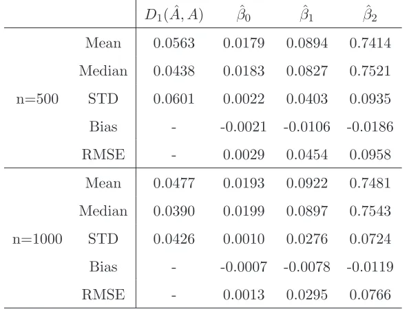
The mean of estimation errors D1(A,A) is less than 0.06 while it decreases over 15% as theˆ sample size increases from 500 to 1000. The negative biases indicate a slight underestimation for the heteroscedastic coefficients. The relative frequencies for ˆr taking different values are listed in Table 2. It shows that when the sample size n increases, the estimation of r becomes more accurate.
5
An application
The Value-at-Risk (VaR) is widely adopted by banks and other financial institutions to mea-sure and manage market risk, as it reflects downside risk of a given portfolio or investment. Specifically, at a given confidence level 1−a, the VaR of a portfolio with weightωt is defined as
the solution to
P(ωt∆Yt< V aRa|Ft−1) =a, (5.1)
where ∆Yt is a vector of log returns of assets in the portfolio. In the case when the conditional
densityf(∆Yt|Ft−1) is normal, (5.1) reduces to the well known formula
V aRa=ωtµy(t) + (ω′tΣy(t)ωt)1/2za, (5.2)
whereza is the a-th quantile of the univariate standard normal distribution.
In this section, we attempt to compare the VaR forecasting results by assuming three different models: AR-DCC, EC-DCC, EC-VF-DCC for the asset price series {Yt}. The DCC refers to
5.1 Data set and estimation of the EC-VF-DCC model
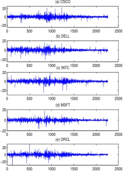
Our data set consists of 2263 daily log prices of CSCO, DELL, INTC, MSFT and ORCL, the five most active stocks in US market, from June 19, 1997 to June 16, 2006. The plots of log returns (in percentage) are presented in Figure 1 which shows significant time-varying volatilities. Descriptive statistics are listed in Table 3. All unconditional distributions of these series exhibit excessive kurtosis and nonzero skewness, indicating significant departure from the normal distribution.
The estimation procedure for the EC-VF-DCC model is given step by step as follows.
Step 1. Fit an error correction model for Yt to determine the structural and cointegration
pa-rameters. Compute the estimate of conditional mean vector ˆµy(t) = ˆΘXt+ ˆγαˆ′Yt−1.
Step 2. Conduct a multivariate portmanteau test for the squared residuals obtained from the previous step to detect conditional heteroscedasticity. If there exists serial dependence, fit a volatility factor model for the residual series{Zt} to determine the factor loading matrix
ˆ
A, otherwise switch to Step 3 with ˆA=Ir and r =d.
DenoteB = (b1, b2,· · · , bd−r), the objective function (3.4) can be modified to
Ψn(B) = τ0
X
τ=1
X
C∈B
w(C)kB′ 1 n−τ0
n
X
t=τ0+1
(ZtZt′−Σˆz)I(Zt−τ ∈C)Bk2
wherew(C)≥0 are weights which ensure that the sum overC ∈ Bconverges. In numerical implementation, we simply takeBas the collection of all the balls centered at the origin in Rd and w(C) ={#(B)}−1.
An algorithm for estimatingB and r is given as follows. Put
Ψ(b) =
τ0
X
τ=1 ˜
Φτ(b), Φ˜τ(b) =
X
C∈B
w(C)[b′ 1 n−τ0
n
X
t=τ0+1
(ZtZt′−Σˆz)I(Zt−τ ∈C)b]2,
Ψl(b) = τ0
X
τ=1
nXl−1
i=1
X
C∈B
w(C)[ˆb′i 1 n−τ0
n
X
t=τ0+1
(ZtZt′−Σˆz)I(Zt−τ ∈C)b]2+ ˜Φτ(b)
o
.
Compute ˆb1by minimizing Ψ(b) subject to the constraintb′b= 1. Forl= 2,· · ·, d, compute ˆbl which minimizes Ψl(b) subject to the constraintb′b= 1,b′ˆbi = 0 fori= 1,2,· · · , l−1. Let ˆr = arg min0≤r≤dP C(r) with ˆBr = (ˆb1,ˆb2,· · · ,ˆbr), where P C(r) is defined by (3.9).
Note that ˆBr′Bˆr=Id−ˆr. Let ˆAconsist of the ˆr(orthogonal) unit eigenvectors, corresponding
to the common eigenvalue 1, of matrixId−BˆrBˆr
Step 3. Fit a dynamic conditional correlation (DCC) volatility model (Engle (2002)) for{Aˆ′Z
t}
and compute its conditional covariance ˜Σz(t) =Dt1/2RtDt1/2.
To this end, we first fit each element ofDt with a univariate GARCH(1,1) model using the
i-th component of ˆA′Zt only, and then model the conditional correlation matrixRt by
Rt=S(1−θ1−θ2) +θ1(εt−1ε′t−1) +θ2Rt−1,
whereεtis a ˆr×1 vector of the standardized residuals obtained from the separate GARCH(1,1)
fittings for the ˆr components of ˆA′Z
t, andS is the sample correlation matrix of ˆA′Zt.
If ˆA=Id, the estimate of conditional covariance matrix ˆΣy(t) of ∆Yt is equal to ˜Σz(t) and
terminate the algorithm. Otherwise proceed to Step 4.
Step 4. The factor structure in (2.1) and the factsB′A= 0, B′e
t=B′Zt, AA′+BB′ =Id lead
to a dynamics for Σy(t)≡Σz(t) as follows
ˆ
Σy(t) = ˆAΣ˜z(t) ˆA′+ ˆAAˆ′ΣˆzBˆBˆ′+ ˆBBˆ′Σˆz, (5.3)
where ˆΣz = n−1τ0
Pn
t=τ0+1ZtZ
′
t.
We determine the cointegration rank by minimizing M(m, k) defined by (3.11). The surface ofM(m, k) is plotted againstmand kin Figure 2. The minimum point of the surface is attained at (m, k) = (1,1), leading to an error correction model for this data set with lag order 1 and cointegration rank 1. Applying the Ljung-Box statistics to the squared residuals, we haveQ5(1) = 63.2724, Q5(5) = 305.7613 and Q5(10) = 633.7103. Based on asymptotic χ2 distributions with degrees of freedom 11, 111 and 236,3 the p-values of these Q statistics are all close to zero. Consequently, the portmanteau test confirms the existence of conditional heteroscedasticity. The algorithm stated in Step 2 leads to an estimator for the number of factors, andP C(r) is plotted against r in Figure 3. Clearly, a two-factor structure (i.e. ˆr = 2 ) is determined for the residual series {Zt}.
5.2 Comparison of Value-at-Risk forecasting results
The VaRs are computed at level 0.05 (denoted by V aR0.05) for the last 1000 trading days of data span. We assume three models: AR-DCC, EC-DCC, EC-VF-DCC for the asset prices
3
The Qd(l) statistic has asymptotically a χ
2
distribution with degree of freedom d2
l−nm,k where nm,k =
d+d2
(k−1) + 2dm−m
2
{Yt}, and four time invariant portfolios with weightsω1 = (1,1,1,1,1)′/5,ω2 = (1,2,3,4,5)′/15,
ω3 = (5,4,3,2,1)′/15, ω4 = (1,3,5,4,2)′/15. To compare the VaR forecasting performances, we calculate failure rates for the different specifications. The failure rate is defined as the proportion of rt =ωt′∆Yt smaller than the VaRs. For a correctly specified model, the empirical failure rate
is supposed to be close to the true level a. Tables 4 display the results for the five percent level. We observe from table 4 that the EC-VF-DCC performs reasonably well, while AR-DCC has a difficulty in providing failure rates close to 0.05. The empirical failure rates for AR-DCC are high, which means that it underestimates the risk. The results for the EC-DCC and EC-VF-DCC model are comparable, but the average computing time for EC-DCC is much longer, see the last column of table 4. This shows that the factor structure imposed on the residual term of an error correction model can improve the computational velocity in high-dimensional problems.
The above results show that the EC-VF model proposed in this paper is a promising tool for risk analysis. First, it incorporate the impact of cointegration which makes the VaR computation more accurate. Secondly, it deduces a high-dimensional optimization problem into a much lower-dimensional problem, thus accelerates the VaR computation to a great extent.
ACKNOWLEDGMENTS
We thank an anonymous referee and the co-editor for their insightful comments and valuable suggestions. Qiaoling Li was partially supported by the National Natural Science Foundation of China. Jiazhu Pan was partially supported by the starter grant from University of Strathclyde, U.K.
References
Andersen, T. G., T. Bollerslev, F. X. Diebold and P. Labys (1999). Realized volatility and correlation. http://www.ssc.upenn.edu/ fdiebold/papers/paper29/temp.pdf
Anderson, H. M., J. V. Issler and F. Vahid (2006). Common features. Journal of Econometrics132, 1-5. Bai, J. S. and N. Serena (2002). Determining the number of factors in approximate factor models.
Econometrica70, 191-211.
Bauwens, L., S. Laurent and J. V. K. Rombouts (2006). Multivariate GARCH models: a survey. Journal of Applied Econometrics21, 79-109
Bollerslev, T. (1986). Generalized autoregressive conditional heteroskedasticity. Journal of Econometrics
31, 307-327.
Duan, J. C. and S. R. Pliska (2004). Option valuation with co-integrated asset prices. Journal of Economic Dynamics & Control28, 727-754
Engle, R. F. (2002). Dynamic conditional correlation - a simple class of multivariate GARCH models. Journal of Business and Economic Statistics20, 339-350.
Engle, R. F. and C. W. J. Granger (1987). Co-integration and error correction: Representation, estimation and testing. Econometrica55, 251-276.
Engle, R. F. and K. F. Kroner (1995). Multivariate simultaneous generalized ARCH.Econometric Theory,
11, 122-150.
Engle, R. F and K. Sheppard (2001). Theoretical and empirical properties of dynamic conditionalcorre-lation multivariate GARCH.A preprint.
Fan, J., M. Wang and Q. Yao (2005). Modelling multivariate volatilities via conditionally uncorrelated components. J. Roy. Statist. Soc. B, accepted.
Ghost, A. (1993). Hedging with stock index futures: estimation and forecasting with error correction model. The Journal of Futures Markets13,743-752
Granger, C. W. J. (1981). Some properties of time series data and their use in econometric model specification. Journal of Econometrics16, 121-130.
Granger, C. W. J. and A. A. Weiss (1983). Time series analysis of error correction models, in Studies in Econometrics, Time Series and Multivariate Statistics, ed. by S. Karlin, T. Amemiya and L.A. Goodman. New York: Academic Press, 255-278.
Kroner, K. and J. Sultan (1993). Time-varying distributions and dynamic hedging with foreign currency futures. Journal of Financial and Quantitative Analysis28, 535-551.
Kupiec, P. (1995). Techniques for verifying the accuracy of risk measurement models. Journal of Deriva-tives2, 173-84.
Li, Q., J. Pan and Q. Yao (2006). On determination of cointegration rank. A preprint.
Lien, D. and X. Luo (1994). Multiperiod hedging in the presence of conditional heteroscedasticity. The Journal of Futures Markets14, 927-955.
Lien, D. and Y. K. Tse (2002). Some recent developments in futures hedging. Journal of Economic Surveys16, 357-396.
Lien, D. (1996). The effect of the cointegration relationship on futures hedging: a note. The Journal of Futures Markets16, 773-780.
Pan, J. and Q. Yao (2007). Modelling multiple time series via common factors. Biometrika,95, 365-379. Pan, J., D. Pe˜na, W. Polonik and Q. Yao (2007). Modelling multivariate volatilities by common factors.
Preprint
Phillips, P. C. B. (1991). Optimal inference in cointegrated systems. Econometrica59, 283-306.
van der Weide, R. (2002). Go-GRACH: a multivariate generalized orthogonal GRACH model. Journal of Applied Econometrics17, 549-564.
van der Vaart, A. W. and J. A. Wellner (1996). Weak Convergence and Empirical Processes. Springer, New York.
Appendix Proofs
The first lemma shows the Φn(r,Bˆr) defined in subsection 3.2 is a non-increasing function of the
number of factors r.
Lemma A.1 If 0≤r1 < r2 ≤d, then Φn(r1,Bˆr1)≥Φn(r2,Bˆr2).
Proof. For 0 ≤ r1 < r2 ≤ d, ˆBr1 can be written as ( ˜Br2,B˜d−(r2−r1)) where ˜Br2 consists of the first d−r2 columns of the matrix ˆBr1. We have
Φn(r1,Bˆr1) = sup 1≤τ≤τ0,C∈B
k( ˜Br2
,B˜d−(r2−r1)
)′Dˆn,τ(C)( ˜Br2,B˜d−(r2−r1))k
= sup 1≤τ≤τ0,C∈B
° ° ° ° ° ˜ Br′
2Dˆ
n,τ(C) ˜Br2 B˜r
′
2Dˆ
n,τ(C) ˜Bd−(r2−r1)
˜
Bd−(r2−r1)′Dˆ
n,τ(C) ˜Br2 B˜d−(r2−r1)
′ ˆ
Dn,τ(C) ˜Bd−(r2−r1)
° ° ° ° ° ≥ sup
1≤τ≤τ0,C∈B
kB˜r′2Dˆ
n,τ(C) ˜Br2k= Φn(r2,B˜r2) ≥ Φn(r2,Bˆr2).
The last inequality holds because ˆBr is the minimizer of Φn(B) in the metric space (HDr, D).
The proof of Theorem 3.2 needs the following two lemmas.
Lemma A.2 For any fixedr withr0 ≤r≤d, there exists aB ∈ HDr such that Φ(r, B) = 0.
For 0≤r < r0, Φ(r, B)>0 holds for all B∈ HrD.
Proof. It is clear that B′A0 = 0 implies Φ(r, B) = 0 from the relation between Φ(r, B) and the factor model with true loading matrixA0.
For r = r0, there must be a matrix in Hr0
D, denoted by Br0, such that Br
′
0A0 = 0, thus
Φ(r0, Br0) = 0 and it reaches the minimum value. We haveBr0 =B0r0 inHr
0
D by Assumption B.
For r0 < r ≤d, let B = Br0
0 H, whereH is an arbitrary (d−r0)×(d−r) matrix such that H′H =I
For any B∈ Hr
D withr < r0,B′A06= 0. If Φ(r, B) = 0, which means that for any 1≤τ ≤τ0 and any C ∈ B, B′D
τ(C)B = 0, by choosing C = Rd, we have B′A0E(FtFt′)A′0B = 0. This is impossible becauseE(FtFt′) is a positive definite matrix.
Lemma A.3 For any 0≤r < r0, there exists aκr>0 such that
p lim
n→∞[Φn(r, ˆ
Br)−Φn(r0,Bˆr0)]≥κr,
where p lim denotes the limit in probability. For anyr0 ≤r < d, it holds that
Φn(r,Bˆr)−Φn(r0,Bˆr0) =Op(
1 √
n).
Proof. It follows from the definition of ˆB that
Φn(r,Bˆr)−Φn(r0,Bˆr0)≥Φn(r,Bˆr)−Φn(r0, B0r0).
Recall that Φ(r0, B0r0) = 0 by Lemma A.2. Hence,
Φn(r,Bˆr)−Φn(r0, Br00)
= [Φn(r,Bˆr)−Φ(r,Bˆr)]−[Φn(r0, B0r0)−Φ(r0, B0r0)] + Φ(r,Bˆr) = Op(
1 √
n) + Φ(r,Bˆ
r)≥O p(
1 √
n) + Φ(r, B
r
0). (A.1)
The second equality holds by the similar way to (3.6) with a slight modification that ˆBris related ton. The last inequality is from the definition ofB0. These imply that, for any 0≤r < r0,
p lim
n→∞[Φn(r, ˆ
Br)−Φn(r0,Bˆr0)]≥κr := Φ(r, B0r),
and from Lemma A.2,κr >0.
For the second part, since
|Φn(r,Bˆr)−Φn(r0,Bˆr0)| ≤ |Φn(r,Bˆr)−Φn(r0, B0r0)|+|Φn(r0, B0r0)−Φn(r0,Bˆr0)|
≤2 max
r0≤r≤d|
Φn(r,Bˆr)−Φn(r0, B0r0)|,
it is sufficient to prove that for anyr0 ≤r ≤d,
Φn(r,Bˆr)−Φn(r0, B0r0) =Op(
1 √
n).
Notice that, from (A.1), Φn(r,Bˆr)−Φn(r0, B0r0) = Op(√1n) + Φ(r,Bˆr). Thus we need to prove
Φ(r,Bˆr) =O
p(√1n) for any r0≤r≤d, where Φ(r,Bˆr) = sup
1≤τ≤τ0,C∈B
For an arbitrary (d−r0)×(d−r) matrixH such thatH′H =Id−r, we have
kBˆr′Dτ(C) ˆBrk
=k( ˆBr−Br0
0 HH′B
r′
0
0 Bˆr+Br
0
0 HH′B
r′
0
0 Bˆr)′Dτ(C)( ˆBr−Br
0
0 HH′B
r′
0
0 Bˆr+Br
0
0 HH′B
r′
0
0 Bˆr)k =k[(Id−B0r0HH′B
r′
0
0 ) ˆBr]′Dτ(C) ˆBr+ (Br
0
0 HH′B
r′
0
0 Bˆr)′Dτ(C)(Id−B0r0HH′B
r′
0
0 ) ˆBrk
where the last equality holds because the relation Br ′
0
0 A0 = 0 implies thatBr ′
0
0 Dτ(C)B0r0 = 0 for any τ ≥1 andC ∈ B. Hence,
kBˆr′Dτ(C) ˆBrk ≤ k(Id−B0r0HH′B
r′
0
0 ) ˆBrkkDτ(C)k(kBˆrk+kB0r0HH′B
r′
0
0 Bˆrk) =D( ˆBr, Br0
0 H)kDτ(C)k(
√
d−r+kBr0
0 HH′B
r′
0
0 Bˆrk) ≤D( ˆBr, Br0
0 H)kDτ(C)k(
√
d−r(1 +d−r)).
Note that Φ(r, Br0
0 H) = 0 by Lemma A.2, that is D(Br
0
0 H, Br0) = 0. Thus D( ˆBr, Br
0
0 H) = Op(√1n). It is easy to see that sup1≤τ≤τ0,C∈BkDτ(C)k =Op(1). Therefore, Φ(r,Bˆ
r) =O p(√1n).
This completes the proof.
Proof of Theorem 3.2. The objective is to verify that limn→∞P(P C(r)−P C(r0)<0) = 0 for all 0≤r≤dand r 6=r0, where
P C(r)−P C(r0) = Φn(r,Bˆr)−Φn(r0,Bˆr0)−(r0−r)g(n).
For r < r0, ifg(n)→0 as n→ ∞,
P(P C(r)−P C(r0)<0) =P(Φn(r,Bˆr)−Φn(r0,Bˆr0)<(r0−r)g(n))→0
because, by Lemma A.3, Φn(r,Bˆr)−Φn(r0,Bˆr0) has a positive limit in probability.
Forr > r0, Lemma A.3 implies that Φn(r,Bˆr)−Φn(r0,Bˆr0) =Op(√1n). Thus, if√ng(n)→ ∞
asn→ ∞, we have
P(P C(r)−P C(r0)<0) =P(Φn(r0,Bˆr0)−Φn(r,Bˆr)>(r−r0)g(n))
=P(√n[Φn(r0,Bˆr0)−Φn(r,Bˆr)]>(r−r0)√ng(n))→0.
Table 1: Simulation results: summary statistics of estimation errors
D1( ˆA, A) βˆ0 βˆ1 βˆ2
Mean 0.0563 0.0179 0.0894 0.7414
Median 0.0438 0.0183 0.0827 0.7521
n=500 STD 0.0601 0.0022 0.0403 0.0935
Bias - -0.0021 -0.0106 -0.0186
RMSE - 0.0029 0.0454 0.0958
Mean 0.0477 0.0193 0.0922 0.7481
Median 0.0390 0.0199 0.0897 0.7543
n=1000 STD 0.0426 0.0010 0.0276 0.0724
Bias - -0.0007 -0.0078 -0.0119
[image:19.595.166.441.436.498.2]RMSE - 0.0013 0.0295 0.0766
Table 2: Relative frequencies for ˆr taking different values, whenr = 1.
ˆ
r 0 1 2 3 4 5 6
n=500 .0120 .8425 .1310 .0105 .0040 0 0
n=1000 .0090 .9765 .0100 .0045 0 0 0
Table 3: Summary statistics of the log-returns
n=2263 CSCO DELL INTC MSFT ORCL
Mean 0.000423 0.000523 1.95×10⁻⁵ 0.0002 0.000418
Stdev 0.031847 0.03027 0.030313 0.023074 0.0364
Min -0.145 -0.20984 -0.24868 -0.16976 -0.34615
Max 0.218239 0.163532 0.183319 0.178983 0.270416
Skewness 0.149215 -0.11826 -0.39156 -0.17347 -0.22637
[image:19.595.138.468.577.723.2]Table 4: Comparison of V aR0.05
ω1 ω2 ω3 ω4 t (Min)
AR-DCC 0.067 (0.001) 0.071 (0.000) 0.065 (0.005) 0.062 (0.032) 287.3
EC-DCC 0.052 (0.659) 0.059 (0.061) 0.051 (0.713) 0.053 (0.268) 294.7
EC-VF-DCC 0.049 (0.713) 0.056 (0.308) 0.053 (0.268) 0.055 (0.312) 41.5
Figures in parentheses are p-values for the Kupiec likelihood ratio test used to compare the
empirical failure rate with its theoretical value, see Kupiec (1995). The average computing time
[image:20.595.179.433.359.717.2]in minute for each model is recorded in the last column.
Figure 1: Plots of daily log-returns (%) of (a)CSCO, (b)DELL, (c)INTC, (d)MSFT and (e)ORCL.
Time span is from June 19, 1997 to June 16, 2006 with 2263 observations.
0 500 1000 1500 2000 2500
−20 0 20
(a) CSCO
0 500 1000 1500 2000 2500
−20 0 20
(b) DELL
0 500 1000 1500 2000 2500
−20 0 20
(c) INTC
0 500 1000 1500 2000 2500
−20 0 20
(d) MSFT
0 500 1000 1500 2000 2500
−20 0 20
Figure 2: Plot ofM(m, k) against the cointegration rankm and the lag orderk
0
1
2
3
4
1 2
3 4
0.5 1 1.5 2
cointegration rank m lag order k
M
(m
,k
)
Figure 3: Plot ofP C(r) against the number of factors r
0 1 2 3 4 5
0.4 0.405 0.41 0.415 0.42 0.425 0.43 0.435 0.44 0.445
the number of factors r
PC
va
lu
[image:21.595.114.473.492.699.2]