Semi-Analytical Solution for the Optimal Low-Thrust
Deflection of Near Earth Objects
Camilla Colombo*, Massimiliano Vasile† and Gianmarco Radice‡ University of Glasgow, Glasgow, G12 8QQ, United Kingdom
This paper presents a semi-analytical solution of the asteroid deviation problem when a low-thrust action, inversely proportional to the square of the distance from the Sun, is applied to the asteroid. The displacement of the asteroid at the minimum orbit interception distance from the Earth’s orbit is computed through proximal motion equations as a function of the variation of the orbital elements. A set of semi-analytical formulae is then derived to compute the variation of the elements: Gauss planetary equations are averaged over one orbital revolution to give the secular variation of the elements, and their periodic components are approximated through a trigonometric expansion. Two formulations of the semi-analytical formulae, latitude and time formulation, are presented along with their accuracy against a full numerical integration of Gauss equations. It is shown that the semi-analytical approach provides a significant saving in computational time while maintaining a good accuracy. Finally, some examples of deviation missions are presented, as an application of the proposed semi-analytical theory. In particular, the semi-analytical formulae are used, in conjunction with a multi-objective optimization algorithm to find the set of Pareto optimal mission options that minimizes the asteroid warning time and the spacecraft mass while maximizing the orbital deviation.
Nomenclature
MOID
A = matrix form of proximal motion equations a = acceleration vector, km/s2
a = semi-major axis, km b = semi-minor axis, km
m
d = diameter of the mirror, m
E = incomplete elliptic integral of the second kind e = eccentricity
r
e = relative error
F = incomplete elliptic integral of the first kind
t
G = matrix form of the Gauss’ equations h = angular momentum, km2/s
i = inclination, deg
sp
I = specific impulse of the spacecraft engine, s j = integer number
k = proportionality constant of the acceleration, km3/s2 M = mean anomaly, deg
d
m = dry mass, kg
* Ph.D. Candidate, Department of Aerospace Engineering, James Watt (South Building), [email protected], Student Member AIAA.
† Senior Lecturer Ph.D., Department of Aerospace Engineering, James Watt (South Building), [email protected], Member AIAA.
0
m = mass into space, kg n = angular velocity, s1
p = semilatus rectum, km r = orbital radius, km
T = transition matrix
NEO
T = asteroid nominal orbital period, s or days t = time, s or MJD since 2000
d
t = departure time from the Earth, s or MJD since 2000
e
t = time when the low-thrust arc ends, s or MJD since 2000
i
t = interception time, s or MJD since 2000
MOID
t = time at the minimum orbit interception distance point, s or MJD since 2000
w
t = warning time, s or MJD since 2000 v = velocity vector, km/s
v = orbital velocity, km/s
α = vector of the orbital parameters
r = vector distance of the asteroid from Earth at the minimum orbit interception distance, km
r = deviation vector in the Hill coordinate frame, km s
= component of the deviation vector, km
v = impulsive maneuver vector, km/s
α = orbital element difference between the perturbed and the nominal orbit
= true anomaly, deg
*
= argument of the latitude, deg
= Sun gravitational constant, km3/s2 = argument of the ascending node, deg
= argument of the perigee, deg Subscripts
h = direction of the angular momentum
n = normal direction in the orbital plane
h = tangential direction in the orbital plane
I.
Introduction
EAR Earth Object (NEO) interception and hazard mitigation has been recognized as a key issue for the safety of life on Earth. The threat posed by asteroid Apophis, with the uncertainties on its orbit after the close encounter with Earth in 2029, has highlighted the importance of space missions aiming at studying NEOs. In particular, tracking the position and velocity of the asteroid and characterizing its shape and composition have become of primary importance in view of any future deviation strategy. Furthermore testing the technology required to deflect an asteroid is now the primary objective of missions such as Don Quijote 1.
The effect of a number of deviation strategies proposed in the past can be modeled as an impulsive variation of the velocity of the asteroid (e.g. kinetic impactor, nuclear explosion). Other strategies, instead, would result into a low thrust applied to the asteroid with a continuous momentum change (e.g. solar collector, pulsed laser, mass driver, gravity tractor, enhanced Yarkovsky effect) 2.
The consequent variation of the orbit of the asteroid can be computed through a numerical procedure and the result has to be validated through orbit tracking and astronomical observations. Carusi et al. 3 studied the δv requirement for deflecting a hazardous near Earth object at different epochs. The orbital course of the asteroid following a deflection impulse along its velocity is computed through the numerical propagation of the full n-body dynamics. They show that, when an encounter occurs before the impact epoch, the required deflection maneuver is noticeably lower than after the encounter itself. Kahle et al. 4 extended this study by removing the assumption of a maneuver along-track; they showed that using a different direction for the deflection maneuver in the vicinity of a planetary encounter increases significantly the performance. The issue with numerical approaches is the
computational time, which becomes a limit when the trajectory has to be integrated over a long period, without losing accuracy. Of course, in the case of a real event, the CPU time would not be an issue; nonetheless, a number of authors have developed analytical formulations, in order to make extensive investigations and gather useful lessons from the computation of a wide range of solutions. In this case the simplification of the two-body problem is often adopted.
Ahrens and Harris 5 gave an estimation of the δv required for deflecting an asteroid from an Earth-crossing orbit and Scheeres and Schweickart 6 derived an analytical expression of the shift in the position of the asteroid, under the assumption of a circular orbit and a constant acceleration aligned with the velocity of the NEO. This strategy, that yields a change in the mean motion of the asteroid, is proposed for long lead time until the impact. Subsequently Izzo 7 proposed a similar solution but extended to non circular orbits. However, this formulation introduces an integral term, which was solved analytically only in the case of an impulsive deflection maneuver. Furthermore, the effect of the deviation strategy is translated in a change of mean motion and hence in a phase shift; other changes in the orbital geometry are not included. A more general approach was used by Conway 8 to determine the near-optimal direction in which an impulsive maneuver should be given. The modified orbital course was propagated analytically forward in time by means of Lagrange coefficients expressed through universal formulae. An analysis on the minimum δv and the optimal impulse angle was performed also by Park and Ross 9, who used Lagrange coefficients to propagate the deviated orbit of the asteroid rather than only its displacement with respect to the nominal course. They also included the effects of the Earth gravity 10,11. Song et al. 12 investigated the deflection of asteroids and comets using a power-limited laser beam. They used the same technique proposed by Park and Ross 9 to solve the heliocentric two-body motion after the laser is shut off, whereas when the laser is on, the trajectory of the Earth crossing object is numerically integrated. They found that the optimal operating angle, between the asteroid velocity and the thrust acceleration vector remains in the range [150 180] degrees for warning times longer than one asteroid period, regardless of the orbital elements of the asteroid.
In this paper, the attention is focused on deviation techniques that make use of a continuous low thrust action. In particular, we perform an extensive search for all mission opportunities, over a wide range of launch dates that are Pareto optimal with respect to three criteria: the achievable displacement of the asteroid at the point of Minimum Orbit Interception Distance (MOID), the time between the launch and the hypothetical impact and the propellant mass for the transfer trajectory. Reconstructing the set of all Pareto optimal solutions requires the evaluation of several tens of thousands of trajectories, thus the numerical computation of the transfer trajectory of the spacecraft and of the deflected trajectory of the asteroid would be impractical.
Since 1950 13-15 several authors have proposed analytical solutions to some particular cases of the low-thrust problem. Tsien14 and Benney15 developed a solution for escape trajectories, respectively subject to radial and tangential continuous thrust acceleration. Following a similar formulation, Boltz 16,17 proposed a solution in the case the ratio between the thrust and the gravity acceleration is kept constant. In both cases, the orbit is assumed to be circular or nearly circular.
Kechichian 18 used an averaging technique to compute analytical solutions for orbits raising with constant tangential acceleration in the presence of Earth shadow. Kechichian’s equations, which contain some terms expanded in power of the eccentricity, are accurate for small to moderate values of the eccentricity, up to 0.2. The effects of the Earth oblateness are also considered. Gao and Kluever 19 adopted an averaging technique with respect to the eccentric anomaly, for continuous tangential thrust trajectories, also accounting for the Earth oblateness and the Earth shadow. The value of the elliptic integrals in the solution of Gao and Kluever is approximated and the accuracy of the solution depends on the eccentricity.
Other analytical solutions for low-thrust trajectories were studied by Petropoulos 20 who presented a general overview of the approximated solutions derived so far. In his work, Petropoulos developed some analytical integrals to describe the secular evolution of the orbit of a spacecraft, subject to different thrust control laws. The rate of change of the orbital energy and the eccentricity are time-averaged and reformulated introducing some elliptic integrals, which are valid for all initial eccentricity from slightly above zero.
The assumption for the analytical developments in this paper is that the deflection strategy uses the Sun as a power source and therefore the thrust acceleration is inversely proportional to the square of the distance from the Sun. Furthermore, we focus our attention on the case in which the thrust is aligned with the tangent to the osculating orbit of the asteroid.
In order to obtain an analytical solution for the variation of the orbital elements, Gauss’ equations are averaged over one orbital revolution. However, the required accuracy for the computation of the miss distance is higher than for the design of a generic low-thrust trajectory, hence, unlike other works 18-20, also the periodic variation of the orbital elements is taken into account. In addition, the analytic integrals are updated with a one-period step to further improve the accuracy. The general applicability of the proposed formulation and their accuracy is demonstrated through a number of test cases. Furthermore, some analyses are presented on the sensitivity of the deviation to the in-plane orbital elements of the nominal orbit of the asteroid. Finally, families of Pareto optimal solutions, for different asteroids will be presented.
II.
Asteroid Deviation Problem
Given the time of interception ti of a generic NEO, the objective is to maximize the minimum orbit interception
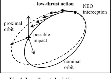
distance from the Earth, by applying a low-thrust deviation action, which consists in a continuous push on the asteroids centre of mass over a certain interval of time. In general, any deviation strategy generates a perturbation of the nominal orbit of the asteroid. The new orbit can be considered proximal to the unperturbed one (see Fig. 1).
Fig. 1 Low thrust deviation maneuver.
If is the true anomaly of the NEO at the MOID along the unperturbed orbit and * the corresponding
latitude, we can write the variation of the position of the NEO, after deviation, with respect to its unperturbed position by using the proximal motion equations 22:
2
3 2
* *
sin
cos sin
1 cos 2 cos cos
sin cos sin
r
h
r ae
s a M a e
a
r r
s e M r e e r i
s r i i
(1)
where sr, s and sh are the displacements in the radial, transversal and perpendicular to the orbit plane
directions respectively, so that the deviation is r
sr s sh
T, and 1e2 . In a matrix form:
tMOID
MOIDr A α (2)
Ta e i M
α is the vector of the orbit element difference at the MOID between the perturbed and the nominal orbit, where M is the mean anomaly. When a low thrust deviation action is applied over
nominal orbit proximal
orbit
possible impact
[image:4.595.201.394.331.468.2]the interval
ti te
, being tetMOID the time when the maneuver is ended, the total variation of the orbitalparameters can be computed by integrating Gauss’ planetary equations 24:
2
*
*
*
2
2
1
2 cos sin
cos
sin sin
1 sin cos
2sin 2 cos
sin
2 1 sin cos
t
t n
h
h
t n h
t n
da a v
a dt
de r
e a a
dt v a
di r a
dt h
d r
a
dt h i
d r r i
a e a a
dt ev a h i
dM b e r r
n a a
dt eav p a
(3)
The low thrust strategy provides an acceleration a
t
at an ah
T, here expressed in a tangential-normal-binormal reference frame, such that at and an are the components of the acceleration in the plane of the osculationorbit respectively, along the velocity vector and perpendicular to it, and ah is the component perpendicular to the orbital plane. Note that the derivative of M, in the 6th equation of system (3), takes into account the instantaneous change of the orbit geometry at each instant of time t
ti te
and the variation of the mean motion due to the change in the semi-major axis along the thrust arc.Letting α
t
a e i M
T to be the vector of the orbital parameters, we define:
Te i
t t a e i M
α α α
the finite variation of the orbital elements with respect to the nominal orbit, in the interval
ti te
, obtained from the numerical integration of Eqs. (3). It is important to point out that M in Eqs. (1) must include the phase shift between the Earth and the asteroid. Therefore, since the mean anomalies at the MOID on the perturbed MMOID andon the nominal orbits MMOID are computed as:
MOID e e MOID e i e MOID e i i p e MOID e
MOID i MOID p
M M t n t t M t M n t t n t t M n t t
M n t t
where tp is the passage at the pericenter, then the total variation in the mean anomaly between the proximal and the unperturbed orbit is:
MOID MOID e i MOID i i e e
M M M n n t n t n t M
(4)
where ni is the nominal angular velocity and
3e
n
a a
The variation of the other orbital parameters in Eqs. (1), instead, is simply a a, e e, i i,
, .
If r
sr s sh
T is the vector distance of the asteroid from the Earth at the MOID and
Tr h
s s s
r is the variation given by Eqs. (1) at tMOID, then the objective function for the maximum deviation problem is:
2
2
2r r h h
s s s s s s
r r (5)
The proximal motion equations provide a very simple and general means to compute the variation of the MOID with good accuracy, without the need for further analytical developments. Compared with methods that are analytically propagating the perturbed trajectory using Lagrange coefficients 9-12, the proposed approach does not require any solution of the time equation for every variation of the orbit of the asteroid and is therefore less computationally expensive. On the other hand, it is conceptually and computationally equivalent to those approaches 8 that are analytically propagating only the variation of position and velocity of the asteroid by using the fundamental perturbation matrix 24. Conversely, the benefit of using proximal motion equations expressed in orbital elements is the explicit relationship between the components of the perturbation action and the geometric characteristics of the orbit of the asteroid.
Gauss’ equations (3), together with Eq. (4), provide a way to compute the variation of the orbital elements between the nominal and the deviated orbit. The equations account both for the geometrical variation of the orbit and the secular change in the mean motion. In order to compute the effect of any low thrust deflection strategy, Gauss’ equations would have to be numerically integrated. However, in section III of this paper we will restrict our attention to the case of a tangential push with modulus inversely proportional to the square of the distance from the Sun. Note that, if we integrated only the first term of the last of Eqs. (3) , neglecting the variations of e, i, ω and Ω, and we inserted it into Eq. (4) we would get:
ei t
e i MOID i i e e t
M n n t n t n t n dt
(6)which is the secular change in the mean motion, already considered by other authors 6,7. The equivalence of Eq. (6) to what already in the literature can be demonstrated as follows. Let us start by re-writing Eq. (6) as:
e ei i
t t
MOID t t
M n t t n dt
and integrating by part:
e
i t
MOID t
dn
M t t dt
dt
(7)Now, the differential dn can be written as a function of da, and through the first of Gauss’ equations (3) as a function of the time shift dt:
5 2
2
3 2 2
t
dn a da
a v
da a dt
Hence, Eq. (7) becomes:
3 e i t
MOID t
t
v
M t t a dt
a
If now we use the superscript ˆ to denote the time coordinates measured from the interception time ti and we take the mean value of the semi-major axis out of the integral, we get:
ˆ
0
3 ˆ ˆ ˆ ˆ
,
e t
MOID
M t t t dt
a
v a which then can be translated M to the variation of the time to encounter induced by the strategy deflection action a, projected onto the velocity of the asteroid 7:
ˆ
0
3 ˆ ˆ ˆ ˆ
,
e t
MOID
a
t t t dt
v a A. Analysis of the Optimal Thrust Direction
An estimation of the optimal direction 23 of the push can be obtained by maximizing the deviation r at the MOID, given the time-to-impact t
tMOIDti
. The deviation vector can be computed as:
tMOID
MOID t
t
tr A G v T v
where T is the transition matrix that links the impulsive v at time t to the consequent deviation at tMOID. AMOID is the matrix in (2) and Gt is the matrix associated to the Gauss’ equations written for finite differences, i.e. the control acceleration being replaced by an instantaneous change in the asteroid velocity vector:
t t
αG v
Following Conway’s 8 approach, r can be maximized by choosing an impulse vector
opt
v parallel to the eigenvector of Τ conjugate to the maximum eigenvalue. As a result of this analysis, we can derive that for a ∆t larger than a specific tNEO1TNEO the optimal impulse presents a dominant component along the tangent direction, being this one associated to the shifting in time between the position of the asteroid and the Earth, rather than to a geometrical variation of the MOID. This conclusion is in agreement with the preliminary analysis on the v direction performed by Ahrens and Harris 5 the numerical verification by Park and Ross 9 and the mathematical demonstration provided by Conway 8. In the case of a low-thrust maneuver, as a first approximation, this results can be generalized by choosing the control vector at time t instantaneously tangent to the optimal impulsive v t . Hence in this work, we focus on low-thrust acceleration in the tangent direction. This is a valid assumption when we consider hazardous cases with a warning time longer than approximately 0.75TNEO. For a better estimation of the
optimal direction of thrust in the case of low-thrust propulsion, one can refer to the analysis by Song et al. 12. Note that, in general, the direction that maximizes r is not optimal for the maximization of r r defined in Eq. (5). However, in this paper we use the maximization of r as an approximation to the general case, since it is valid for an actual impact, i.e. MOID equal to zero.
III.
Semi-Analytical Formulae for Low-thrust Deviation Actions
In this section, a set of semi-analytical formulae will be derived to calculate the total variation of the orbital parameters due to a low-thrust action. It is considered that a continuous acceleration at is applied along the orbit
track, with modulus given by:
2 t
k a
r
where r is the distance from the Sun and k is a time-invariant proportionality constant that has to be fixed according to the specification of the power system. The selection of this acceleration law does not represent a severe restriction to the mission design, in fact Eq. (8) describes any strategy that exploits the Sun as a power source, e.g. a solar electric propulsion spacecraft that rendezvous with the NEO, anchors to its surfaces and pushes, or a solar mirror which collects the energy from the Sun and focuses it onto the asteroid surface to ablate it. Moreover, if the formulae presented in the following are adopted to design a low-thrust trajectory, Eq. (8) represent the control acceleration due to a power-limited spacecraft.
Gauss’ equations are written as a function of the true latitude *:
* *
d d dt
dt d d
α α
where, in case of zero acceleration out-of-plane ah,
*
2
d h
dt r
(9)
where h is the orbital angular momentum. Under the hypothesis of planar tangential maneuver, Eqs. (3) become:
2 2
*
2
*
*
*
2
*
2 2
*
2
1
2 cos
0
0 1
2sin
2 1 sin
t
t
t
t
da a v r a h d
de r
e a
v h
d di d d d
d r
a
ev h
d
dM b e r r
n a
eav p h
d
(10)
Eqs. (10) are averaged over one period of the true anomaly 24, yielding the average rate of change of the orbital parameters:
,2 2
* *
0
1 2
d d
d
d d
α α
The total variation α of the orbital elements over one orbital period of * can be approximated as: ,2
2
* 0
d d d
α
αif a zero variation in the anomaly of the pericenter is assumed, i.e. d*d. This assumption holds true in the case
the deviation is calculated over one integer number of orbital revolutions, because the periodic variation of is zero and the secular one is of order 1011 rad for the level of acceleration used in this paper. Thus the variation of
0 0 0 0 0 0 2 2 22 2 2
2 2 2 2 2 2 2 2 1 cos 2
1 2 cos
1
2 1 2 cos
1 0
0
sin 1 1
2
1 2 cos
1 2 1 1
sin
1 cos 1 2 cos
e
e k d
h e e
a e
k a e e
a d
h a e
i
a e
k d
eh e e
n a e bk a e
M
h e eah e e
0 0 2 2 22 sin 1 1
1 cos 1 2 cos
ebk a e
d
ah e e e
By considering a and e constant within one revolution, the following analytical formulae can be derived after some algebraic manipulations:
0 0 0 0 0 0 0 0 0 0 2 2 2 2 , 2 2 , 2 , 2 , 12 4 4
1 E , 1 F ,
2 1 2 1
4 2 E ,
2 1 2
0 0
1 2 cos
2 1 2arctan 1 e e e e e e e
k e e
e e e
h ev e e
e v e a k a h i e e k eh ev e M e 0 0 0 0 2 2 , 2 2 2 , 1 sin tan
2 1 cos
2arctan 1 2 cos
2 1 2 cos
1 e e e e e e v a e e
bk e e
e
eah ve v e
(11)
where:
2
2
1 2 cos
1 e e v a e
2
2
1 2 cos
1
e e
e
Eqs. (11) contain two elliptic integrals to be evaluated only once every orbital period:
2
20
4
F , where F ,
2 1 1 sin
e d
e
(12)
is the incomplete elliptic integral of the first kind and:
2 2
0
4
E , where E , 1 sin
2 1 e
d e
(13)
the incomplete elliptic integral of the second kind 24,25. Note that the integral kernels (11), to be evaluated in
0 2
and 0, are function only of the semi-major axis and the eccentricity.
The variation of the mean anomaly M strongly influences the consequent deviation, calculated through Eqs. (1). Hence, when the primitive function is evaluated in the upper limit 02, the value of the eccentricity is set equal
to e e, in order to have a better approximation of M in Eqs. (11). This allows taking into account the secular variation e over one orbital revolution. Finally, the total variation of the orbital parameters over the thrust-arc is determined by integrating Eqs. (11) with the Euler method with a step size of one orbital period.
A. Accuracy Analysis
The accuracy of Eqs. (11) was assessed by computing the relative error on the achieved deviation r between the numerical propagation of Gauss’ equations and the analytical formulae:
propagated analytical r
propagated
e
r r
r .
The deviation r is calculated considering a push of the asteroid over the angular interval * *
0 0 j2
,
with j an integer number and by calculating the resulting displacement right at the end of the thrust arc. The vector
analytical
r is the deviation obtained by means of the analytical formulae (11), while rpropagated was computed through
the numerical integration of Gauss’s equations (10):
* 0 * 0
2
* * j
d d d
α
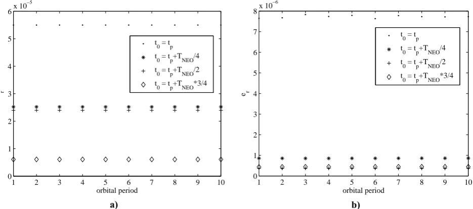
αFig. 2a represents the relative error on the computation of the deviation of Apophis, when pushing over an increasing number of orbital revolutions and starting the deviation maneuver at different angular positions. In fact the variation of the orbital parameters over one orbital revolution depends on where, along the orbit, the maneuver starts. In the legend tp is the time at the pericenter, t0 the time when the deviation action commences and TNEO is
the asteroid nominal orbital period. Fig. 2b shows the relative error for an asteroid with higher eccentricity and inclination (e0.73, i25). An adaptive step-size Runge-Kutta Fehlberg integrator was used for the numerical integration and the absolute and the relative tolerance were set to 1 10 16 and 2.3 10 14 respectively in order to
1 2 3 4 5 6 7 8 9 10 0
1 2 3 4 5
6x 10
−5
orbital period
e r
t
0 = tp
t
0 = tp+TNEO/4
t
0 = tp+TNEO/2
t
0 = tp+TNEO*3/4
a)
1 2 3 4 5 6 7 8 9 10
0 1 2 3 4 5 6 7
8x 10
−6
orbital period
e r
t
0 = tp
t
0 = tp+TNEO/4
t
0 = tp+TNEO/2
t
0 = tp+TNEO*3/4
b)
Fig. 2 Relative error on the deviation. a) Asteroid Apophis. b) Asteroid 1979XB.
Other than the accuracy, an advantage of the analytical formulation is a significant reduction in the computational cost with respect to a numerical integration through a Runge-Kutta method. In fact, the CPU time§ required for the numerical propagation of Gauss’ equations is one order of magnitude higher than the one required for the computation of the analytical formulae, as reported in Table 1.
Table 1 Computational time of the analytical and numerical approach.
orbital periods time analytical [s] time numerical [s] percentage of saving in computational time (analytical/numerical)
1 4.3e-003 5.6e-002 92.3
2 6.1e-003 7.2e-002 91.5
3 6.8e-003 9.9e-002 93.1
4 9.3e-003 1.2e-001 92.2
5 1.2e-002 1.4e-001 91.7
6 1.3e-002 1.7e-001 92.0
7 1.6e-002 1.9e-001 91.7
8 1.9e-002 2.1e-001 91.1
9 2.0e-002 2.3e-001 91.2
10 2.2e-002 2.5e-001 91.2
IV.
Periodic Variation of the Orbital Parameters
The analytical formulation in Eqs. (11) describes the mean variation of the keplerian elements, hence it gives a sufficiently accurate estimate of their variation over one full revolution of the true latitude. For smaller angular intervals, the periodic component of the perturbation must be included because its variation is not zero. To this aim an expression was derived to estimate the periodic component of semi-major axis, eccentricity and argument of the perigee. The trend of a, e, function of * can be approximated by the Eqs (14):
[image:11.595.77.545.121.328.2] [image:11.595.93.502.430.572.2]
* * * * * * *
0 0 0
* * * * * * *
0 0 0
* * * * * * *
0 0 0
sin sin 2 sin sin 2 cos cos 2
a p a p
e p e p
p p
a
a a C C
e
e e C C
C C
(14)
In Eqs. (14) the first two terms are the initial condition for the secular evolution at point 0 (i.e. the point when the deviation action commences), the third term indicates the secular variation obtained form Eqs. (11) and the forth one is the periodic variation. The coefficients Ca, Ce and C are the amplitudes of the periodic variation. Their value
was set through a calibration process: Gauss’ equations in Eqs. (10) were numerically integrated over one orbit of
*
. Said anum, 2, enum, 2 and ωnum, 2 the vectors resulting form the numerical integration of Eqs. (10), then we
have:
* *
2 , 2 0 0
* *
2 , 2 0 0
* *
2 , 2 0 0
2 2 2 num num num a a e e a a e e ω ω (15)
from which the amplitudes of the periodic components can be computed as:
* * * * * * 2 2 2 2 2 2 max min 2 max min 2 max min 2 a e C C C a a e e ω ω (16)where * * *
0 0 2
. Since Eqs. (15) come from a numerical integration, this calibration process is time consuming. However it needs to be performed once and for all, given the asteroid and the proportionality constant of the acceleration k. In fact it was verified that for low-thrust action the amplitude of the periodic components of the perturbation is almost constant over a number of integration periods that are sufficient to deviate the asteroid by a considerable distance.
250 300 350 400 450 500 550 600 0,191034
0,191035 0,191036 0,191037 0,191038 0,191039 0,19104 0,191041 0,191042 0,191043 0,191044
* [deg]
e(
*)
Apophis
*
0 = *(tp+TNEO/4)
numerical semi-analytical mean
Fig. 3 Semi-analytical expression of the eccentricity. Asteroid Apophis.
Table 2 Maximum relative error between the numerical and semi-analytical integration. Asteroid Apophis Asteroid 1979XB
eccentricity 1.3e-006 1.4e-007
semi-major axis 3.5e-008 8.2e-008
anomaly of the pericenter 6.9e-007 6.6e-008
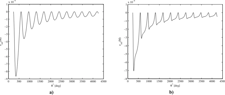
In order to properly take into account the periodic variation of the mean anomaly within an interval smaller than one revolution, the corresponding Gauss’ equation has to be integrated over *:
2 2
* 2 1 sin t
dM b e r r
n a
eav p h
d
(17)
in which e
* , a
* and
* are expressed through Eqs. (14). The relative error on M with respect to the fullintegration of Eqs. (10) is represented in Fig. 4a and Fig. 4b:
0 500 1000 1500 2000 2500 3000 3500 4000 4500
−9 −8 −7 −6 −5 −4 −3 −2 −1 0
1x 10
−8
θ*
[deg]
erel
(M)
a)
0 500 1000 1500 2000 2500 3000 3500 4000 4500
−8 −7 −6 −5 −4 −3 −2 −1 0
1x 10
−8
θ*
[deg]
erel
(M)
b)
[image:13.595.172.405.114.288.2] [image:13.595.97.498.335.385.2] [image:13.595.87.536.507.697.2]Note that introducing the periodic terms allows for the computation of the evolution of the orbital elements starting from any angular position along the orbit. In fact, if the point when the deviation action commences (i.e. point 0 in Eqs. (14)) is different form the pericenter, the initial mean parameters are different from the initial osculating elements. The periodic terms instead assure that the required accuracy for a deviation maneuver starting at any angular position. This would have not been achieved by using other formulations 18-20 that account only for the secular variations.
V.
Time Formulation
In some applications the semi-analytical formulae introduced in section III and IV are enough to describe a low-thrust trajectory. The variation of the orbital parameters over an integer number of full revolutions of the angle *
can be calculated directly from Eqs. (11); for the last revolution, the periodic components are counted together with the secular variations through Eqs. (14). This approach, called latitude formulation in thefollowing, does not use the time as independent variable. It allows a considerable saving in computational time and at the same time it provides good accuracy, comparable with a numerical integration with low tolerance.
However, the time is required when dealing with the asteroid deviation problem since the component of the deviation associated to the shift in time has to be taken into account. In fact the latitude formulation accounts only for the shift in position of the asteroid. Given the thrust arc
ti te
, we want to apply the described semi-analytical formulation in order to find the displacement of the asteroid after a given time. Eqs. (11) are used to compute the variation of the orbital elements over the number of full revolutions contained in the time interval
ti te
. Whereas,for the remainder of the thrusting arc, the element differences are calculated using Eqs. (14) and (17). The interval
*
corresponding to the time interval
ti te
is computed by numerically integrating Eq. (9). Note that the termscorresponding to the secular variation of the parameters in Eqs. (14) are calculated updating a, e and at each orbital revolution.
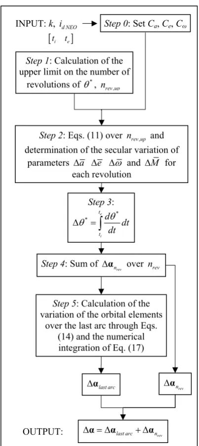
Given the asteroid identification number id NEO and the proportionality constant of the acceleration k, the
calibration procedure gives the amplitude of the periodic component of a, e and (Step 0). Once computed, the values of Ca, Ce and C are kept constant for every t
ti te
and for every interval
ti te
. The algorithmproceeds with the calculation of the upper limit on the number of revolutions contained in the interval
ti te
; thequotient of the division between
teti
and the nominal period of the asteroid is rounded to the nearest integertowards infinity (Step 1). In fact due to the perturbation introduced by the low-thrust action, the time to perform a full revolution of * is different from the one of the unperturbed orbit. For each revolution, the value of the secular
variation of the orbital parameters is computed with Eqs. (11) (Step 2), updating at each integration step (which is one period long) a, e, and recalculating the elliptic integrals (12) and (13). Once the secular variations are available (Step 3), the value of * corresponding to the thrust arc and the exact number of revolutions are computed through
Eq. (9), with the orbital parameters computed through Eqs. (14). The secular variations of the parameters calculated in step 2 are added up over the number of full revolutions (Step 4), while the calculation of the variation of the orbital elements in the reminder of the thrust arc is performed through the evaluation of Eqs. (14) and the integration of Eq. (17) (Step 5). Note that a
* , e
* and
* , given by Eqs. (14), are calculated updating the values ofa
Fig. 5 Time formulation algorithm.
A. Accuracy Analysis
The accuracy of the time formulation was verified by computing the relative error er time formulation, between the deviation ranalytical tf, , calculated through the algorithm in Fig. 5, and the deviation rpropagated tf, , computed with the
numerical integration of Eqs. (3):
, ,
,
, propagated tf analytical tf r time formulation
propagated tf
e
r r
r Step 3:
*
* e
i t
t
d dt dt
Step 4: Sum of
rev n
α over nrev Step 1: Calculation of the
upper limit on the number of revolutions of *,
, rev up
n
Step 5: Calculation of the variation of the orbital elements
over the last arc through Eqs. (14) and the numerical integration of Eq. (17)
last arc
α
rev last arc n
α α α
OUTPUT: INPUT: k, id NEO
ti te
Step 2: Eqs. (11) over nrev up, and determination of the secular variation of
parameters a e and M for each revolution
rev n
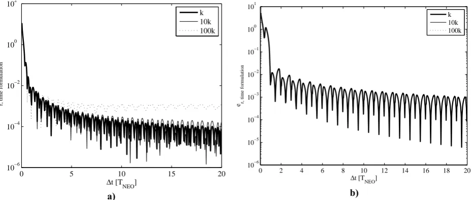
[image:15.595.197.399.100.552.2]The relative error was computed for increasing values of the proportionality constant k. Fig. 6a and Fig. 6b report
,
r time formulation
e calculated with the nominal value of k (set in section VI), 10k and 100k, respectively for asteroid Apophis and 1979XB. The values of er time formulation, are plotted against the push time teti, which was set equal to the time-to-impact t (i.e. te tMOID).
0 5 10 15 20
10−6
10−4
10−2
100
102
Δt [T
NEO]
e r, time formulation
k 10k 100k
a)
0 2 4 6 8 10 12 14 16 18 20
10−6 10−5 10−4 10−3 10−2 10−1 100 101
Δt [TNEO]
er, time formulation
k 10k 100k
b)
Fig. 6 Relative error of the time formulation. a) Asteroid Apophis (k=2.2·105 km3/s2). b) Asteroid 1979XB (k=2·104
km3/s2).
The high value of the relative error when t 1TNEO is due to the approximation, introduced with the periodic
components of the orbital elements in Eqs. (14). For t 1TNEO the difference between orbital elements of the
perturbed and the nominal orbit α is of the same order of magnitude of the approximation error of the periodic components. As a consequence the relative error difference of the orbital elements
, ,
, propagated tf analytical tf r
propagated tf
e
α α
α
α
[image:16.595.80.546.185.382.2]0 2 4 6 8 10 12 14 16 18 20
10−6
10−5
10−4
10−3
10−2
10−1
Δt [T
NEO]
e r
(
δ
M)
a)
0 2 4 6 8 10 12 14 16 18 20
10−6
10−5
10−4
10−3
10−2
10−1
100
101
Δt [TNEO] er
(
δ
M)
b) Fig. 7 Relative error on δM. a) Asteroid Apophis. b) Asteroid 1979XB.
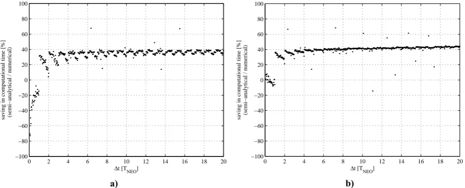
Hence the time formulation can be substituted to the numerical integration only for a thrust arc t longer than one orbital revolution. On the other hand, when low-thrust strategies are selected, the thrust arc is in general longer than 1 TNEO. Fig. 8 depicts the percentage of saving in computational time of the semi-analytical approach, with time
formulation, with respect to the numerical integration. When t 1TNEO the gain is around 40% and it increases
with the length of the push arc.
0 2 4 6 8 10 12 14 16 18 20
−100 −80 −60 −40 −20 0 20 40 60 80 100
Δt [T NEO] saving in computational time [%] (semi−analytical / numerical)
a)
0 2 4 6 8 10 12 14 16 18 20
−100 −80 −60 −40 −20 0 20 40 60 80 100
Δt [T NEO] saving in computational time [%] (semi−analytical / numerical)
b)
Fig. 8 Percentage of saving in computational time by using the semi-analytical time formulation with respect to the numerical integration of Gauss’ equations. a) Asteroid Apophis. b) Asteroid 1979XB.
VI.
NEO Deviation Missions
[image:17.595.82.546.111.309.2] [image:17.595.74.546.430.621.2]in Table 3, together with the minimum orbit interception distance and the mass of the asteroid. The MOID r was calculated using the Earth’s ephemerides on 27 January 2027 at 12:00 hrs, taken from analytic ephemerides which approximate JPL ephemerides de405**. Note that, the actual MOID varies with time 26, due to the actual orbit of both the Earth and the asteroid. On the other hand, the aim of this work is not to reproduce any specific and realistic impact scenario, but rather to assess the performance of a low-thrust deviation action over a wide range of mission opportunities. A more accurate calculation of the MOID would produce a more precise estimation of the actual achievable deviation but would not invalidate the results in this paper.
Table 3 Asteroids orbital and physical parameters.
Asteroid Semi-major axis [AU] eccentricity Inclination [deg] MOID [km] Mass [kg]
Apophis 0.922 0.191 3.331 30706 4.6·1010
1979XB 2.350 0.726 25.143 3725733 4.4·1011
As a reference case, we consider a spacecraft equipped with a solar mirror with a diameter of 100 m and a dry mass md
27 of 895 kg. The spacecraft is launched at a time
d
t , selected in a range of 20 y before the possible collision, with maximum hyperbolic excess velocity is 3.5 km/s, and is equipped with engine delivering an unlimited thrust with an Isp 3000 s. Once the spacecraft has intercepted the asteroid, the low thrust deviation maneuver is performed from ti up to the time at the MOID (i.e. te tMOID); no propellant is assumed to be consumed during the
deviation phase, but a 25% margin on the total wet mass is considered, to account for station keeping and mirror deployment operations. Table 4 summarizes the key parameters of the mission.
Table 4 Mission characteristics.
sp
I 3000 s
m
d 100 m
d
m 895 kg
margin on m0 25%
,max
v 3.5 km/s
tMOIDtd
max 20 yThe value of k was set according to the model of the solar collector developed in Ref. 28. The value of k was chosen in order to obtain the same order of acceleration provided by a solar inflatable mirror, with a diameter dm of between 100 and 110 m, along the range of distances from the Sun covered by the asteroid during its motion. Fig. 9 compares the acceleration computed through the full model described in Ref. 28, against Eq. (8), over a feasible range of distances for asteroid Apophis. Between the orbit apocentre and pericenter, Eq. (8) (solid line) gives an acceleration comparable with the one calculated through the full solar collector model (dash lines). Note that Eq. (8) does not take into account the decrease of the mass of the asteroid due to the ablation of the material.
[image:18.595.65.530.207.243.2] [image:18.595.220.376.361.462.2]0.7 0.75 0.8 0.85 0.9 0.95 1 1.05 1.1 0.6
0.8 1 1.2 1.4 1.6 1.8 2 2.2
2.4x 10
-11
r [AU]
at
[k
m
/s
2]
a (dm=100 m)
a (dm=110m)
k/r2
Fig. 9 Magnitude of the acceleration for Apophis.
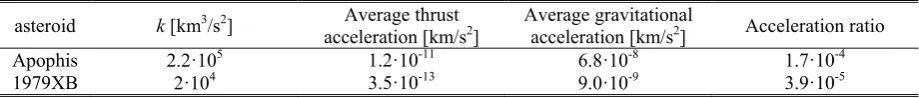
Table 5 reports the values of the acceleration constant k for each asteroid, together with the average of the thrust acceleration on a nominal orbit of the asteroid, according to Eq. (8), the average of the Sun gravitational acceleration and the ratio between the two accelerations.
Table 5 Acceleration constant and average of the accelerations acting on the asteroid. asteroid k [km3/s2] Average thrust
acceleration [km/s2] Average gravitational acceleration [km/s2] Acceleration ratio
Apophis 2.2·105 1.2·10-11 6.8·10-8 1.7·10-4
1979XB 2·104 3.5·10-13 9.0·10-9 3.9·10-5
A multi-objective optimization was performed to minimize the vector objective function:
0
min m tw r r r (18)
with respect to the launch date, the time of flight and the hyperbolic excess velocity. In Eq. (18) m0 is the wet mass
at the Earth defined as:
0 d p 1.25
m m m
where mp is the propellant mass for the transfer. twtMOIDtd is the warning time and r r is the total deviation to be maximized. The transfer trajectory was calculated through a shape-based method 21,29 and a hybrid optimization approach, blending a stochastic search with an automatic solution space decomposition technique 30,31, was used for the solution of problem in Eq. (18).
A. Apophis Deviation Mission
[image:19.595.200.385.106.263.2] [image:19.595.68.528.343.392.2]20000 3000 4000 5000 6000 7000 8000 9000 10000 200
400 600 800 1000 1200
t
d [MJD2000]
[image:20.595.185.401.110.275.2]ToF [d]
Fig. 10 Launch opportunities for a deviation mission to Apophis.
The launch dates and transfer times in Fig. 10 correspond to the set of Pareto optimal solutions in Fig. 11a. In Fig. 10 we can see that a wide range of launch opportunities are available every year between 2010 and 2030, though the required transfer time might change significantly. In particular we can identify two groups of solutions around 5000 MJD2000 and 7500 MJD2000 with a short transfer time (i.e. short warning time), a scattered set of solutions with a transfer time between 500 and 600 days and three groups of solutions with long transfer time. Note that we used a non-exhaustive stochastic search process, therefore more solutions can exist in the same range of launch dates. In Fig. 11a, the three axes represent the components of the objective function Eq. (18); the z-axis contains the magnitude of the deviation r . The mass into space m0, that was limited to 5000 kg in this analysis,
is a function of the mass of propellant required to perform a transfer from the Earth to the asteroid. In the case of Apophis a mission using a solar collector with a diameter of 100 m, would achieve deviations of the order of 106 km, in a time range of 20 years of warning time, while solutions with 1000 days of warning time have a deviation of about 20000 km.
The modulus of the achieved deviation is proportional to the length of the thrust interval t tMOIDti and it has a periodic trend with the angular position of the point of interception, as shown in Fig. 11b. The gray scale represents the value of the true anomaly (in degrees) at interception.
1000 2000
3000 4000
5000
0 2000 4000 6000 8000
0 2 4 6
x 106
m
0 [kg]
t
w [d]
||
[image:20.595.81.541.491.696.2]δ
r|| [km]
a)
0 1000 2000 3000 4000 5000 6000 0
1 2 3 4 5 6
x 106
Δt [d]
||
δ
r|| [km]
−150 −100 −50 0 50 100 150
b) Fig. 11 Deviation mission to Apophis.
Now, neglecting the transfer phase and assuming the same value of the acceleration constant k, the sensitivity of the deviation to the in-plane orbital elements a, and e of the nominal orbit of the asteroid can be investigated. Several values of semi major-axis and eccentricity are considered, covering the range of in-plane elements for a group of 338 Aten asteroids from the JPL catalogue††. The range for semi-major axis in AU is 0.64
0.99 a
and
the range for eccentricity is 0.013 e 0.89. For each value of eccentricity and semi-major axis the corresponding orbit is computed keeping the other orbital elements equal to the parameters of Apophis. The deviation is calculated for increasing values of the pushing time, from 1 d up to 20 years before the date at the corresponding MOID.
The modulus of the deviation of the asteroid at the MOID is displayed in Fig. 12a as a function of the pushing time. Note that, as a consequence of the acceleration law, which goes with the inverse of the distance from the Sun, the achievable deviation for a fixed warning time decreases with the increase of the nominal semi-major axis. This is clear if we analyze the first equation of Eqs. (3) and we substitute the value of the acceleration:
2
2
2 da a v k dt r
In fact, this term is proportional to a1 2 and is the term which mostly influences the value of the deviation,
because it contributes to the shift in time.
As we can appreciate, from Fig. 12b, the relative error with the precise numerical integration does not exceed 10 -2, which means that the accuracy of the analytical formulae is good in the selected range of values of the semi-major axis.
0.650.7
0.750.8
0.850.9
0.951
0 2000 4000 6000 8000
0 2 4 6 8 10 12 14
x 106
a [AU]
Δt [d]
||
[image:21.595.79.544.363.577.2]δ
r|| [km]
2 4 6 8 10 12
x 106
a)
0.65 0.7 0.75 0.8 0.85 0.9 0.95 1 0
2000 4000
6000 10−7
10−6 10−5 10−4 10−3 10−2 10−1
a [AU]
Δt [d]
e r, time formulation
0 0.002 0.004 0.006 0.008 0.01 0.012
b)
Fig. 12 Sensitivity of the deviation to the semi-major axis. The white line represents Apophis case (a = 0.922 AU).
a) Deviation achieved for orbits with different values of semi-major axis and for increasing values of thrust interval. b) Relative error for different values of semi-major axis.
The sensitivity analysis to the eccentricity, instead, is shown in Fig. 13. In this case (see Fig. 13a), for the same pushing time, the magnitude of the deviation increases, with the increase of the eccentricity. Also the fluctuations within the orbital period are more visible. The local maxima correspond to an interception point prior to the pericenter.
It is very interesting to note that a good accuracy is assured also for different values of eccentricity, within the range 0.013 e 0.89. Fig. 13b shows the relative error of the time formulation. Note that the accuracy of the time
formulation is in general lower than the accuracy of the latitude formulation. In fact, the former one needs a further operation, which is the determination of the value of * corresponding to the thrust arc and the exact number of
revolutions (see Step 3 in Fig. 5).
0 0.2
0.4 0.6
0.8 1
0 2 4 6 8 10
0 1 2 3 4 5 6 7 8
x 106
e
Δt [T
NEO]
||
[image:22.595.80.546.163.383.2] [image:22.595.187.408.548.717.2]δ
r|| [km]
1 2 3 4 5 6 7 x 10⁶
a)
0 0.2 0.4 0.6 0.8 1 0
2 4
6 8
10 10−7
10−6 10−5 10−4 10−3 10−2 10−1
e
Δt [T
NEO]
er, time formulation
0.005 0.01 0.015 0.02 0.025
b)
Fig. 13 Sensitivity of the deviation to the eccentricity. The white line represents Apophis case (e = 0.191).
a) Deviation achieved for orbits with different values of eccentricity and for increasing values of thrust interval. b) Relative error for different values of eccentricities.
B. 1979XB Deviation Mission
The launch opportunities for a deviation mission to asteroid 1979XB are represented in Fig. 14. The test case close approach occurs on the 20th of May 2030 (11097 MJD2000). In this case, the launch opportunities are grouped in single stripes with an average transfer time ranging between around 200 and 800 days. The corresponding set of Pareto optimal solutions is shown in Fig. 15a, which shows that the maximum achieved deviation is of the order of 105 km, since the mass of the asteroid is 4.4 10 11 kg, significantly higher than the mass of Apophis.
30000 4000 5000 6000 7000 8000 9000 10000 11000 100
200 300 400 500 600 700 800 900 1000
t
d [MJD2000]
ToF [d]
The high eccentricity of the orbit of the asteroid 1979XB emphasizes the periodicity of the achievable deviation with t (see Fig. 15b where the grey scale indicates the angular position at interception). The considerable step in the value of the deviation is in correspondence of an interception prior to the pericenter. This effect is amplified for this asteroid, since its orbit is highly elliptical.
1000 2000
3000 4000
5000
0 2000 4000 6000 8000
0 1 2 3 4 5
x 105
m
0 [kg]
t
w [d]
||
[image:23.595.80.544.183.389.2]δ
r|| [km]
a)
0 1000 2000 3000 4000 5000 6000 70000
0.5 1 1.5 2 2.5 3 3.5 4 4.5 5
x 105
Δt [d]
||
δ
r|| [km]
−150 −100 −50 0 50 100 150
b) Fig. 15 Deviation mission to 1979XB.
a) Pareto front. Launch mass, warning time and magnitude of the deviation are represented on the three axes. b) Achieved deviation as a function of the time length of the thrust arc.
Again we performed the same analysis of sensitivity to the semi-major axis and the eccentricity, by computing the deviation for a range of a and e and by keeping the other parameters equal to the one of 1979 XB, which belongs to Apollo class. While the range of the eccentricity is always 0.013 e 0.89, for the semi-major axis a range of 1.0006 a 3.595 AU was considered, as the range of semi-major axis of the Apollo class, taken from the JPL catalogue‡‡.
Also in this case (see Fig. 16a) the value of the deviation, for a fixed pushing time, decreases with the increase of the semi-major axis (the 1979XB case is represented in white line). The different shape with the orbital period, with respect to Fig. 12a is due to the higher eccentricity (e = 0.726).
Finally, the accuracy is represented in Fig. 16b. The relative error, despite being always under 3·10-2, increases with the semi-major axis, for fixed value of the pushing time.
1 1.5 2 2.5 3 3.5 4 0 2000 4000 6000 8000 0 2 4 6 8 10 12 14
x 105
a [AU]
Δt [d]
[image:24.595.83.545.108.318.2] [image:24.595.90.544.450.673.2]|| δ r|| [km] 2 4 6 8 10 12
x 105
a) 1 1.5 2 2.5 3 3.5 4 0 2000 4000 6000 8000 10−6 10−5 10−4 10−3 10−2 10−1 a [AU]
Δt [d]
er, time formulation
0 0.005 0.01 0.015 0.02 0.025 0.03 0.035 0.04 0.045 b)
Fig. 16 Sensitivity of the deviation to the semi-major axis. The white line represents 1979XB case (a = 2.350 AU).
a) Deviation achieved for orbits with different values of semi-major axis and for increasing values of thrust interval. b) Relative error for different values of semi-major axis.
The sensitivity to eccentricity is depicted in Fig. 17. As already observed in Fig. 13a, for the same pushing time, the magnitude of the deviation increases with the increase of the eccentricity (see Fig. 17a). Also in this case a good accuracy is achieved for different values of eccentricity, within the range 0.013 e 0.89. Fig. 17b shows the relative error of the time formulation.
0 0.2 0.4 0.6 0.8 1 0 1 2 3 4 5 6 0 2 4 6 8 10 12
x 105
e
Δt [TNEO]
|| δ r|| [km] 1 2 3 4 5 6 7 8 9 10 11 x 105
a) 0 0.2 0.4 0.6 0.8 1 0 1 2 3 4 5 6 10−6 10−5 10−4 10−3 10−2 10−1 e
Δt [T
NEO] er, time formulation
0 0.005 0.01 0.015 0.02 0.025 b)
Fig. 17 Sensitivity of the deviation to the eccentricity. The white line represents 1979XB case (e = 0.726).