Through-life modelling of nano-satellite power system dynamics

Stephen (2013) Through-life modelling of nano-satellite power system

dynamics. In: 64th International Astronautical Congress 2013, 2013-09-23

- 2013-09-27. ,

This version is available at

https://strathprints.strath.ac.uk/45063/

Strathprints is designed to allow users to access the research output of the University of Strathclyde. Unless otherwise explicitly stated on the manuscript, Copyright © and Moral Rights for the papers on this site are retained by the individual authors and/or other copyright owners. Please check the manuscript for details of any other licences that may have been applied. You may not engage in further distribution of the material for any profitmaking activities or any commercial gain. You may freely distribute both the url (https://strathprints.strath.ac.uk/) and the content of this paper for research or private study, educational, or not-for-profit purposes without prior permission or charge.

Any correspondence concerning this service should be sent to the Strathprints administrator: [email protected]

The Strathprints institutional repository (https://strathprints.strath.ac.uk) is a digital archive of University of Strathclyde research outputs. It has been developed to disseminate open access research outputs, expose data about those outputs, and enable the

IAC-13-C3.4.4

THROUGH-LIFE MODELLING OF NANO-SATELLITE POWER SYSTEM DYNAMICS

Christopher Lowe

University of Strathclyde, UK, [email protected]

Malcolm Macdonald

University of Strathclyde, UK, [email protected]

Steve Greenland

Clyde Space Ltd, UK, [email protected]

This paper presents a multi-fidelity approach to finding optimal, mission-specific power system configurations for CubeSats. The methodology begins with propagation of the orbit elements over the mission lifetime, via a continuous-time model, accounting for orbital perturbations (drag, solar radiation and non-spherical geo-potential). Analytical sizing of the power system is then achieved at discrete long-term intervals, to account for the effects of variations in environmental conditions over the mission life. This sizing is based on worst case power demand and provides inputs to a numerical assessment of the in-flight energy collection for each potential solar array deployment configuration. Finally, two objective functions (minimum deviation about the orbit average power and maximum average power over the entire mission) are satisfied to identify the configurations most suitable for the specific mission requirement. Most Nano-satellites are designed with relatively simple, static-models only and tend to be over-engineered as a result, often leading to a power-limited system. The approach described here aims to reduce the uncertainty in energy collection during flight and provide a robust approach to finding the optimal solution for a given set of mission requirements.

I. INTRODUCTION

A general method is required to aid the Systems Engineer in the design and optimisation of power system configuration, specifically the configuration of deployed solar arrays on board a CubeSat. These Nano-scale platforms are growing in popularity, but more importantly are growing in capability, resulting in them becoming increasingly power-limited. The problem is worsened by fact that traditionally, design of a CubeSat power system during early design phases has been achieved through analytical sizing of the solar arrays and batteries based on estimated orbit-average power demands. This approach is characterised by significant levels of uncertainty and thus, increased safety margins are required resulting in over-engineered solutions. To remedy this, use of multi-fidelity modelling early on can help the designer better understand performance characteristics over the lifetime and arrive at an optimal solution with confidence. This reflects, to a certain degree, the process employed during early phase studies of traditional space missions, where individual sub-system teams would meet to share information and then develop discipline-specific static and dynamic models to assess sub-system performance.

I.I. State of the Art

Calculation of the energy collected by a set of solar cells on-board a spacecraft has been a topic of consideration for many years1, 2, 3 and can be considered

trivial only in the case where cell orientation remains fixed with respect to the Sun (e.g. via gimbal-type mechanisms). For Nano-satellites, and in particular CubeSats, the combination of low Earth orbit (LEO) and orientation-fixed solar cells generally means energy collection is variable over time and is affected greatly by geometric shading (in the case of deployed appendages). These two factors suggest that numerical methods must be applied to obtain a solution in the general case; however analytical, closed-form methods can be applied in specific cases4. More recently, research has been conducted on power profile modelling specific to various classes of small satellites5 and CubeSats6, but tends to be on a mission-specific/trajectory restricted basis.

I.II. Overview of Work

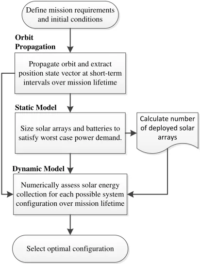
solar arrays are illuminated when the platform is in view of the sun. Battery capacity is also sized at each discrete point and the worst case complete power system (maximum required cell area and battery capacity) is carried forward as the baseline system design. The area requirement is transformed into the necessary number of deployed panels and a database of all possible array configurations (panel combinations and deployment angles) is constructed (§III.II). For each deployment configuration, a dynamic model is employed to analysis the energy collection over a single orbit (using discrete short-term (ST) intervals) at the start of each LT interval (§III.III). Total energy collected by the solar arrays is calculated for each orbit (accounting for discontinuities such as eclipse and panel shading) and stored for use in the optimisation. The final stage in the process (§III.IV) is to find the optimal configuration based on solving a user-defined objective function (Fobj). The Fobj is arbitrary, since it operates on data from the entire solution space. The general flow of the methodology is illustrated in figure 1.

Define mission requirements and initial conditions

Size solar arrays and batteries to satisfy worst case power demand.

Numerically assess solar energy collection for each possible system configuration over mission lifetime

Select optimal configuration Propagate orbit and extract position state vector at short-term

intervals over mission lifetime

Static Model

Dynamic Model Orbit Propagation

Calculate number of deployed solar

arrays

Fig. 1: Flow diagram showing general design methodology and use of multi-fidelity modelling

II. BACKGROUND

In this section, fundamental concepts critical to the success of this work are described. These include analytics associated with performance and design of the power system and time domains employed throughout the modelling process.

II.I. Solar Cell Performance

The rate of solar energy collection from a solar cell is approximately proportional to the cosine of the angle ( ) between the cell normal and cell-Sun vector, commonly known as the incidence angle (for angles less than 90°). Solar energy collection rate can therefore be defined by the following expression, when the satellite is in sunlight.

[1]

Where Acell is the area of the solar cell, S is the solar constant (at 1AU ≈ 1366W) and cell is the cell energy conversion efficiency. During eclipse, the energy collection will be zero and the effects of penumbra partial eclipse are neglected in this work for simplicity (for low earth orbits, these effects are negligible and can be ignored).

II.II. Power System Design

The average power available to a satellite from the solar arrays is an important input to the system design. It must be sufficient to satisfy the total power demand during sunlight, which is the sum of the sub-system power demand (Psun) and the power required for re-charging of the batteries (Pcharge).

[2]

Pcharge is dependent on the power demand during eclipse (Peclipse), eclipse duration ( eclipse), sunlit duration (sun) and total battery charge efficiency ( charge). Failure to comply with the above inequality would result in steady discharge of the battery, which would ultimately lead to mission objectives being sacrificed or complete mission failure in the long term.

[3]

Average power (Pave) can also be defined as:

Where;

[5]

The above expression is discontinuous in the general case due to eclipse conditions, solar cell anti-solar pointing and panel shading. These events are difficult to determine analytically in the general case (especially for elliptical orbits and non-constant rates of attitude variation), so numerical methods are required.

Another major element of any spacecraft power system is the secondary power source, typically batteries. Battery capacity ( bat) can be expressed as a function of some of the parameters used previously and another critical design parameter, the Depth of Discharge (DOD), which is battery-type dependent.

[6]

Battery capacity is related to cost and mass in such a way that it contributes significantly to the design. Typically, an upper limit will be applied in order to restrict dependency on the batteries and maintain compliance with other requirements.

II.III. CubeSat EPS Configuration

The CubeSat standardised geometry is important to the success of this work, since variables such as deployed panel location, orientation and deployment angle can be easily discretised, thus limiting configuration possibilities. Throughout this work, it is assumed that the CubeSats have a 3U form factor (current maximum for P-POD deployment system7), but this is not necessary and other geometries could be employed.

The physical configuration of a CubeSat with deployed panels can be generalised in the following way; first assume that deployable panels are stowed, prior to deployment, against a main body face, f, where f F, (F represents the set of faces available for stowage). Deployment of a panel f is made about an edge k, where kf Kf (Kf is the set of edges surrounding face f). The number of faces and number of edges surrounding a face are defined as nF and nK respectively. Constraints are imposed such that no two panels may be stowed against, or deployed about, the same face or edge, respectively (for any specific configuration).

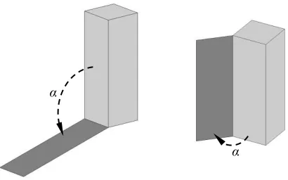
Practically, panels can be deployed by any desired angle, , but again the variable is discretised to between

min and max, at intervals of (figure 2).

[7]

II.III.

Fig. 2: Showing angle of deployment for stowed panels.

Where;

[8]

The final variable required to fully describe a CubeSat system with deployed panels is the number of deployed panels present, np. In this work, , but a more complex structure on which additional deployed panels exist would be feasible also.

In the general case, a combination of the above parameters will result in a specific configuration, c, where c C (C is the full set of available configurations). The number of configurations (nc) possible for system with np deployed panels, is:

[9]

Where n‟ is the total number of configurations possible, irrespective of edge-constraint compliance, and m is the number of non-compliant configurations.

[10]

[11]

Here q is the number of different combinations of stowed face arrangements, represented by Pascal’s formula for nF and np and yp represents the number of deployment edge combinations that result in a non-compliant configuration.

[12]

considered beyond the scope of this paper, but has been verified numerically by the authors.

For all results shown in this paper, the parameters selected are nF = 4 and nK = 4 and result in the following (assuming n = 3*) (Table 1):

Number of deployed panels (np)

Number of possible configurations (nc)

0 1

1 48

2 828

3 6048

4 15714

Table 1: Number of solar array configurations resulting from different numbers of deployed panels

II.IV. Time Domains

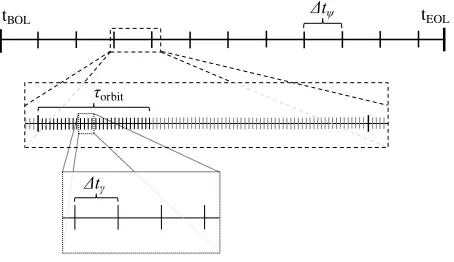
The multi-fidelity modelling approach described here is driven by the use of multiple time-scales. Duration of the orbit propagation is for the lifetime of the mission ( life), and the state variables (orbit elements) are recovered at steps with a fixed short-term (ST) interval ( t). This discrete-time data is used as an input to the static and dynamic models described later. The static model accepts data at long-term (LT) intervals ( t ) on the order of days, and the power system is sized at the start of each interval (t ). This approach is considered sufficiently accurate to capture secular variations caused by the orbit perturbations described above. A special case exists in the form of a fully maintained Sun-synchronous orbit, whereby the orbital and eclipse periods remain constant. For the dynamic model we conduct analysis using ST intervals for a single orbit, beginning at the start of each LT interval. This enables assessment of the spacecraft attitude, panel-panel shading and eclipse effects on solar energy collection. Figure 3 illustrates the various time domains used within the models.

III. METHODOLOGY III.I. Orbit Propagation

Since the objective of this methodology is to find an optimal solution to the configuration problem over the mission lifetime, we must have knowledge of the flight behaviour over this time. Environmental phenomena, such as eclipse duration and beta angle†, may vary significantly during operations, which must be accounted for in the sizing of the power system.

*

The angles possible for a value of n = 3 are 90°, 135° and 180°. An additional interval, say 90°, 120°, 150°, 180° would add significant complexity to the problem, for example increase nc= 4 from 15714 to 49664.

† _{Beta angle is defined as the angle between the}

satellite orbit plane and the Earth-Sun position vector.

Fig. 3: Time domain definition (from mission-scale to short-term interval scale)

Orbit characteristics are captured over the mission lifetime by solving the Gaussian form of Lagrange’s planetary equations of motion, written in modified equinoctial elements8, using a Runge-Kutta Ordinary Differential Equation (ODE) solver implemented in Matlab®. This approach allows application of perturbations to various orders of fidelity, such as non-spherical geo-potential, Solar Radiation Pressure (SRP) and atmospheric drag, so that long-term projections can be made with sufficient accuracy for design purposes. Other perturbations, such as 3rd body gravity effects, are not included in this work for simplicity, however they could be included without a significant increase in computational requirement. Since the majority of Nano-satellites do not feature orbit control/station-keeping capabilities, and area to mass ratio is generally high in comparison to their larger counterparts, it is considered vital that drag and SRP effects are included.

III.II. Static Model

At the start of each LT interval (figure 3), the minimum required solar array area is calculated using:

[13]

Where is defined from equation 2 and varies with time depending on the eclipse duration for the orbit in question. A new parameter is introduced, referred to as energy collection efficiency ( ), which is the ratio of solar array area contributing to energy collection and total array area9. Energy collection efficiency is dependent on array configuration, operational attitude and beta angle. For a nadir pointing system, can vary between 0.05 and 0.35. Therefore, by selecting a value of 0.27, it is likely that some, but not all, of the configurations will meet power demand. Those that do not meet demand (identified during the dynamic modelling phase) will be considered infeasible and discarded, whilst feasible solutions will be carried through and considered in the optimisation phase.

t

orbit

tEOL

The maximum value of , found via equation 13, represents the baseline area necessary for successful operations over the lifetime. The number of deployed panels (np) is then selected such that the actual array area is equal to, or greater than this minimum. The area represented by the complete complement of solar arrays is dependent on the area assigned to each surface. For example, sensors, payload cut-outs and mechanisms may render certain parts of the structure unavailable for solar array placement. In this work, it is assumed that complete photovoltaic coverage of the four largest body panels and complete coverage of both sides of all deployable panels is possible, with no coverage on the two smaller body panels (i.e. emulating the presence of camera and antenna payloads at each end). A packing factor ( pack) of 0.8 is applied throughout to account for geometric inefficiencies.

In addition to sizing the solar arrays at the start of each LT interval, the batteries are sized using equation 6, where again, the worst-case design is considered the baseline (i.e. the largest required capacity).

III.III. Dynamic Model

Upon completion of the static modelling phase, analysis is conducted on each configuration for the given number of deployed panels to assess dynamic flight behaviour over a single orbit at the start of each LT interval, t . The rate of solar energy collection is calculated for each configuration, c, via a modified version of equation 1:

[14]

Where Aarray,proj,n is the projected area of solar array, n, in the plane perpendicular to the spacecraft-sun direction. This projected area is computed numerically and incorporates the effects of anti-solar pointing, eclipse and shading from other panels. Shading effects and anti-solar pointing are calculated prior to operation of the dynamic model by computing the sunlit area of each array for multiple discrete Sun locations assigned to a database of solar azimuth & elevation angles on the spacecraft attitude sphere10. During the simulation, projected cell area at each time, t , is found by rounding the actual solar azimuth & elevation to the nearest associated database grid point. Interpolation between points is intended for future work to decrease error in this approximation.

III.IV. Optimisation Problem

The optimisation problem is formulated for two objective functions:

1. Minimise the set of mean average absolute deviations about the orbit average power over

the entire lifetime. In other words, the system which shows the lowest average fluctuation between the solar array Pmax and Pmin over an orbit, thus representing the most stable system:

[15]

2. Maximise the mean of the orbit average power over the entire mission lifetime. I.e. the system which collects the most energy on average: [16]

Subject to the following constraints: [17]

[18]

[19]

[20]

[21]

[22]

Constraint 17 ensures that a sufficient area of solar array is employed to satisfy the power demand at all discrete times during the mission analysed by the static model. Constraint 18 prohibits the use of more than the maximum allowable number of deployable panels‡. Constraint 19 ensures the battery capacity does not exceed limits imposed in the system requirements. Constraint 20 ensures that no two panels are stowed against the same face prior to deployment, while constraint 21 ensures no two panels are deployed about the same edge. Constraint 22 ensures that no configuration with which energy collection does not meet the demand is carried forward as a feasible solution. I.e. compliance with this condition ensures a positive orbit-averaged flow of energy into the satellite. For the first objective function ( ), the absolute deviation (Di) of a point xi about a central data point m defined as: [23]

‡ _{Importantly, this combination of constraints (17 &}

While the mean average absolute deviation, is the average of all the deviations on the entire set of data, X (x1, x2…xn).

[24]

Specific to this work, the central data point, m, is represented by the orbit average power from the solar arrays (time dependent) and the data points, x, are represented by the instantaneous power (energy collection rate) measured at each ST time step ( ) over each orbit at the start of each LT interval ( ). It can be expressed completely as:

[25]

Where n is equal to the total number of intervals t over the orbit with its epoch at time t . This is effectively a measure of the range between maximum and minimum power from the solar arrays over that particular orbit. To satisfy the objective function, the average of this parameter over the entire set of LT intervals must be calculated, providing a general measure of the power system stability.

[26]

Here, m represents the number of LT intervals over the mission lifetime.

For the second objective function ( ), the orbit average power Pave is found over the orbit at each LT interval, for each configuration, using equation 4, and then the set of these results are averaged over the mission lifetime.

[27]

RESULTS

Analysis was conducted on two typical CubeSat trajectories, the first being deployment from the International Space Station, on 21st July 2012§ and the second a Sun Synchronous orbit with a repeat ground track after 3 days (44 orbits), starting on 27th Sept 2013. Both simulations feature systems that operate in the Nadir attitude mode with the following common parameters:

§

Analogous to the deployment of TechEdSat from Jaxa’s Kibo module.

Symbol Value Unit Description

- 3 U CubeSat form-factor

M 3.6 Kg Mass

CD 2.1 - Drag coefficient 1.9 - Reflectivity constant cell 25 % Solar cell efficiency pack 80 % Cell packing efficiency charge 90 % Battery charge efficiency DOD 20 % Depth of discharge Table 2: Common simulation characteristics

IV.I. ISS Deployment

The following characteristics were used, specific to deployment from the ISS (table 3):

Symbol Value Unit Description rp 405 km Perigee altitude i 51.6 ° Inclination e 0.0027 - Eccentricity

Psun 10 W Ave power demand (sun) Pecl 5 W Ave power demand (eclip)

life 0.5 yr Mission lifetime

t 1 days LT interval

t 1 s ST interval

n 3 - No. deploy angle options Table 3: Characteristics for ISS deployment

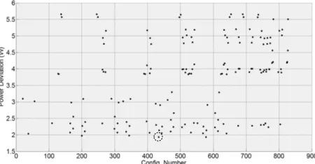
From the parameters defined in table 3, results indicate that a system with 2-deployed solar arrays and a battery capacity of 17.75Whrs would be required to satisfy the general demand. The mission average power and deviation are shown for each feasible configuration, with the optimal solution circled in each.

Fig. 5: Mission average power from feasible solutions deployed from ISS

It is noteworthy that whilst a configuration that provides a satisfactory level of average power/deviation may be selected based purely on experience and design intuition, the likelihood of selecting an optimal solution is negligible. Only through analysis of the available configuration options with a dynamic model is one in a position to appreciate the variability in performance.

The configuration which best satisfies the objective function of minimum deviation (equation 15) is number 434 (figure 6), while that which meets the maximum average power (equation 16) is number 828 (figure 7).

Fig. 6: Optimal configuration (no. 434) displaying minimum average power deviation

Fig. 7: Configuration (no. 828) displaying maximum orbit average power

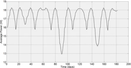
Figures 8 & 9 show development of the orbit average power during the 6 month mission, for configurations 434 & 828 respectively. The periodic drops in average power every ~18days are the result of the regression of the line of nodes, which varies at ~5°/day at this inclination. The depth of this drop in power is due to the coupling effects of nodal regression and Earth-Sun rotation on energy available for collection.

Fig. 8: Orbit average power (configuration no. 434) vs. time over the mission lifetime

Fig. 9: Orbit average power (configuration no. 828) vs. time over the mission lifetime

IV.II. Sun Synchronous Orbit

The characteristics used, specific to the Sun synchronous orbit case, are detailed in table 4. Results indicate that a system with 4-deployed solar arrays and a battery capacity of 17.13Whrs is required to satisfy the general demand. The mission average deviation (figure 10) and average power (figure 11) is shown for each feasible configuration, with the optimal solution circled in each.

Min deviation - Config. No. 434 - Deviation = 1.93W - Ave Power = 15.99W

Symbol Value Unit Description rp 679 km Perigee altitude i 98.1 ° Inclination e 0.0 - Eccentricity

Psun 17 W Ave power demand (sun) Pecl 5 W Ave power demand (eclip)

life 1 yr Mission lifetime

t 5 days LT interval

t 2 s ST interval

n 1** - No. deploy angle options Table 4: Characteristics for Sun sync trajectory

Fig. 10: Power deviation from feasible solutions deployed into Sun synchronous orbit

Fig. 11: Mission average power from feasible solutions deployed into Sun synchronous orbit

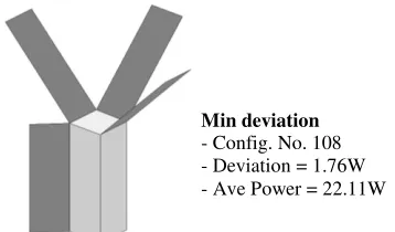
The configuration which best satisfies the objective function of minimum deviation is number 108 (figure 12), while that which meets the maximum average power is number 100 (figure 13).

**

Restricted to a deployment angle of 135° from the stowed position.

Fig. 12: Configuration (no. 108) displaying minimum average power deviation

Fig. 13: Configuration (no. 100) displaying maximum orbit average power

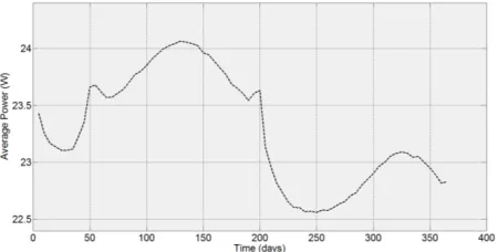
Figures 14 & 15 show development of the average power over the 12 month mission for configurations 108 & 100 respectively.

Fig. 14: Orbit average power (configuration no. 108) vs. time over the mission lifetime

Min deviation - Config. No. 108 - Deviation = 1.76W - Ave Power = 22.11W

Fig. 15: Orbit average power (configuration no. 100) vs. time over the mission lifetime

V. CONCLUSIONS

The procedure presented in this paper outlines a multi-fidelity, multi-step methodology that guarantees the optimal power system configuration required to satisfy a user-defined objective. The incorporation of multiple analysis stages reduces the computational effort required to complete the resource-expensive element of the process, the dynamic simulation. Furthermore, search of the entire solution space means that the global optimum is guaranteed, but to the detriment of analysis speed.

Two 3U CubeSat mission cases were analysed, a 6 month ISS deployed trajectory and a 1 year Sun synchronous trajectory, and the configurations which offered optimal performance in terms of both minimum deviation of power about the orbit average and maximum orbit average power over the mission lifetime were identified.

VI. FUTURE WORK

Improvements in the definition of energy collection efficiency, for various attitude modes and deployed panel numbers, is required to ensure the methodology is flexible for any mission case. For example, a Sun-tracking attitude would be capable of meeting power demand with significantly less solar cell area than is required for a continuously variable attitude, necessitating a higher value for . It is therefore

possible to rapidly assess the effect of different operational attitude modes on energy collection. Through association of cost with respect to deployed panel numbers and battery capacity requirements, integration of the static model into a global system would enable trade-off between system performance and power system cost. For example, payload performance for a sun-tracking attitude may be significantly below that of a magnetically aligned system, but require fewer deployed panels and hence lower system cost.

The introduction of platonic solids into the method of calculating effective area related to solar azimuth and elevation will significantly reduce the number of grid points required to build the matrix required and reduce computation time accordingly. It is here that the vast majority of time is spent, having to build the area projection matrix for each configuration. To compound matters, it is clear that as the number of deployed panels and deployable angle options increase, the number of configuration options increase also. The time required to complete an entire analysis is almost directly proportional to the number of configuration options such exist, efficiencies gained in this element would be highly beneficial.

Interpolation between grid points on the attitude sphere is considered necessary to increase accuracy of the energy collection rate during each short term interval. At present, the solar position is rounded to the nearest grid point, at each time step, resulting in an discretised power profile. The results are considered acceptable for this early phase of study, but should be improved for future investigations.

While a search of the entire design space guarantees finding the optimal solution for the constraints enforced by the user, it demands significant computational resource. Use of global optimisation methods may significantly reduce computation, but still provide a near-optimal solution. It is expected that over-coming the highly stochastic nature of the geometry coupling problem will be the greatest hurdle, but would equally provide greatest benefit in terms of analysis speed.

1

Cho, B. Lee, F, 1988, “Modeling and Analysis of Spacecraft Power Systems”, IEEE Transactions on Power Electronics, Vol. 3, No. 1

2

Capel, A. et al, 2002, “Dynamic Performance Simulation of a Spacecraft Power System”, Space Power; Proceedings of the sixth European Conference

3

Kordon, M. Wood, E. 2003, “Multi-Mission Space Vehicle Subsystem Analysis Tools”, IEEE Aerospace Conference, Proceedings, Vol. 8

4

Anigstein, P. et al, 1998, “Analysis of Solar Panel Orientation in Low Altitude Satellites”, IEEE Transactions on Aerospace and Electronic Systems, Vol. 34, No. 2

5

Paw, C. Varatharajoo, R. 2009, “Solar Profile Prediction for Low Earth Orbit Satellites”, Jurnal Mekanikal, No. 28

6

7

Mitskevich. A, 2011, “Program Level Poly-Picosatellite Orbital Deployer (PPOD) and CubeSat Requirements Document”, Launch Services Program , NASA

8

Walker, M. Owens, J. & Ireland, B. 1985, “A Set of Modified Equinoctial Elements”, Celestial Mechanics, Vol. 36, p. 409-419

9

Lowe, C. 2013, “CubeSat Energy Collection Efficiency: Analysis via Monte Carlo Methods”, Internal Technical Note (pending public release)

10