The spectrum of the Neumann matrix with zero modes

      

City, University of London Institutional Repository

Citation

:

Feng, B., He, Y. and Moeller, N. (2002). The spectrum of the Neumann matrix with zero modes. Journal of High Energy Physics, 2002(038), doi:

10.1088/1126-6708/2002/04/038

This is the unspecified version of the paper.

This version of the publication may differ from the final published

version.

Permanent repository link:

http://openaccess.city.ac.uk/832/

Link to published version

:

http://dx.doi.org/10.1088/1126-6708/2002/04/038

Copyright and reuse:

City Research Online aims to make research

outputs of City, University of London available to a wider audience.

Copyright and Moral Rights remain with the author(s) and/or copyright

holders. URLs from City Research Online may be freely distributed and

linked to.

City Research Online: http://openaccess.city.ac.uk/ [email protected]

arXiv:hep-th/0202176v2 20 Mar 2002

Preprint typeset in JHEP style. - HYPER VERSION MIT-CTP-3243

hep-th/0202176

The Spectrum of the Neumann Matrix with Zero

Modes

Bo Feng, Yang-Hui He and Nicolas Moeller

Center for Theoretical Physics,

Massachusetts Institute of Technology, Cambridge, MA 02139, USA

fengb,yhe,[email protected]

Abstract: _{We calculate the spectrum of the matrix M}′ _{of Neumann coefficients of the Witten}

vertex, expressed in the oscillator basis including the zero-mode a0. We find that in addition to the

known continuous spectrum inside [₋1

3,0) of the matrix M without the zero-modes, there is also an

additional eigenvalue inside (0,1). For every eigenvalue, there is a pair of eigenvectors, a twist-even and a twist-odd. We give analytically these eigenvectors as well as the generating function for their components. Also, we have found an interesting critical parameter b0 = 8 ln 2 on which the forms

of the eigenvectors depend.

Contents

1. Introduction 1

2. Notations and Some Known Results 3

2.1 Properties of the Matrix M 3

2.2 The Matrix of our Concern: M′ ₄

3. One Simple Example 5

4. Diagonalising M′_{: Setup and Continuous Spectrum 6}

4.1 The Continuous Spectrum 8

5. The Determinant: the Functions Aee and Aoo 10

5.1 The FunctionAee 10

5.2 The FunctionAoo 12

6. The Discrete Spectrum 14

6.1 The Case ofλ=₋1/3 14

6.2 Other Solutions atλ 6=−1/3 17

7. The Generating Function 17

7.1 The Twist-even States 18

7.2 The Twist-odd States 19

8. The spectrum of M′12 _{and M}′21 ₂₀

9. Discussions and Conclusions 20

1. Introduction

and so have been the proofs of other conjectures, such as the equality between the algebraic and the geometric sliver, or the form of the pure-ghost kinetic operator around the stable vacuum.

These proofs all came up very recently, shortly after Rastelli, Sen and Zwiebach solved the spectrum of the matrixM of Neumann coefficients [9]. They found that the spectrum is continuous in the range [−1

3,0); every eigenvalue in this interval is doubly degenerate, except for − 1

3 which is

single and twist-odd. They gave a complete solution by finding the density of eigenvalues and the expressions of the corresponding eigenvectors. This result turned out to be a key tool for doing exact calculations in VSFT. Indeed, using the form of the spectrum ofM, Okuyama [10] proved that the ghost kinetic operator of VSFT is given by the ghost fieldcevaluated at the string midpoint, as was already expected [11, 6]. Then in another paper [12], Okuyama also gave an algebraic proof that the D-brane descent relation is correctly reproduced. The ration of the tension of a Dp-brane to the tension of a D(p+ 1)-brane can be expressed in terms of determinants of matrices of Neumann coefficients

R = Tp

2π√α′_Tp+1 =

3Vrr

00 +2b 2

√

2πb3

det(1−M′₎34(1 + 3M′) 1 4

det(1−M)34(1 + 3M) 1 4

, (1.1)

whereM is the matrix formed by the Neumann coefficients of the vertex in the oscillator basis with zero momentum, whereas M′ _{is made out of the Neumann coefficients of the vertex expressed in} the oscillator basis including the zero-mode oscillatora0. The parametre b is an arbitrary constant

in the definition aµ0 := 12 √

bpµ_{− √}1

bix

µ _{[2]. Although it seems, at a first look, that one needs the}

spectrum of both M and M′ _{to calculate R, Okuyama [12] found an elegant way of calculating this} ratio knowing only the spectrum of M. At last, Okuda [13] proved the equality of the geometric sliver and the algebraic sliver [2, 5, 14, 15, 16, 17].

Because the spectrum of M is such an important piece of data, it is reasonable to expect that knowing the spectrum ofM′ _{will be very useful as well. In this paper we thus solve the problem of} finding all eigenvalues and eigenvectors of M′_.

We summarize our results here: We find that the eigenvalues of M′ _{are given by two types,} a continuous and a discrete spectrum. The continuous eigenvalues are the same as that of M

and are located in the range [₋1/3,0). The discrete eigenvalue is located in the range (0,1) and is determined by (5.4) (or (5.5)) implicitly. The corresponding eigenvectors are as follows. For every eigenvalueλ ∈[−1/3,0), we have two degenerate eigenvectors which can be written as a twist-even (4.29) and a twist-odd (4.30). Note that this degeneracy includes the point λ = ₋1/3. For the discrete eigenvalue λ _∈(0,1), we have again two degenerate eigenvectors, a twist-even (6.6) and a twist-odd (6.7). They do not have corresponding analogues inM and consist only of certain vectors

|vei and |voi defined in (2.10).

Interestingly, we have found a critical value b0 = 8 ln 2 ≈ 5.54518 where the forms of the

eigenvectors differ slightly for b _≥ b0 and b < b0. When b < b0, the eigenstates for the continuous

spectrum ((4.29) and (4.30)) can be considered as deformations of those of M by |vei and |voi.

When b _≥ b0, all eigenvectors are as above except at one point λ0 ∈ [−1/3,0) determined by (5.4)

the matrices M ad M′ _{which are key to our derivations. Then, after a review of the method of} diagonalisingM in Section 3, we reduce the central problem of diagonalisingM′ _{into a linear system} of equations in Section 4, wherein we also present the continuous spectrum. In Section 5, we discuss the analytic evaluations and behaviour of zeros of the determinant of the linear system. Sections 6 is the highlight of the paper where we carefully analyse the discrete spectrum ofM′_{. In Section 7 we} evaluate the so-called generating functions explicitly to obtain the components of the eigen-vectors. Finally in Section 8, we apply our methods to analyse the spectra of the other M′rs _{matrices. We}

end with conclusions and prospects in Section 9.

2. Notations and Some Known Results

In this section, we recall some known results and fix the notation we shall use throughout the paper. All relevant results can be found in [9, 10, 12]. We emphasize here that we take α′ _{= 1.}

2.1 Properties of the Matrix M

We first recall the definition of the matrixM, defined as a product of thetwist matrixCmn and

the Neumann Coefficients V11

mn for the star product in open bosonic string field theory:

(M)_mn :=CV11

mn; Cmn:= (−1) m_δ

mn.

In [9], it was found that the eigenvectors of M can be written as

|ki= (v₁k, v₂k, v₃k, ...)T, (2.1) with eigenvalue

M(k) =₋ 1 1 + 2 coshπk

2

. (2.2)

The components vk

i can be found from the generating function

fk(z) =

+∞

X

n=1 vk

n

√ nz

n ₌ 1

k(1−e

−karctanz_{). (2.3)}

We can simplify notations by defining the inner product [10]

hz|ki ≡ +∞

X

n=1 znv_nk,

where _|z_{i ≡}(z, z2_{, z}3_{, ....)}T _{and hz| =|zi}T

is the transpose of _|z_i (not hermitian conjugate). Then the generating function becomes

fk(z) =hz|E−1|ki=hk|E−1|zi (2.4)

where Enm=√nδnm. Under the twist action ofC defined above, we have

The eigenvector |ki has very good properties, most notably the orthogonality under the inner product[12]:

hk_|p_i=_N(k)δ(k₋p), _N(k) := 2

k sinh( πk

2 ). (2.6)

Using this result, we see that |ki forms a complete basis and

1=

Z +∞

−∞ dk

|k_{i h}k_|

N(k) (2.7)

2.2 The Matrix of our Concern: M′ The matrix we try to diagonalize is [2, 12]

M′ = M00′ M0′m

M′

n0 Mnm′

!

=





1− 2 3

b

β −

2 3

√

2b β hve|

−2 3

√

2b

β |vei M +

4 3

(−|veihve|+|voihv0|)

β



, (2.8)

where we have defined

β =V00rr+ b

2 = ln 27 16+

b

2,

|vei=E−1|Aei, |voi=E−1|Aoi,

(Ae)n =

1 + (−)n

2 An, (Ao)n=

1−(−)n

2 An, and An is defined as the coefficients of the series expansion

1 +ix

1−ix

1/3

= X

n=even

Anxn+i

X

n=odd

Anxn. (2.9)

There are a few results concerning the states _|vei and |voi which we will use later. We quote

them from [12] as

hk_|vei=

1

k

cosh(πk

2 )−1

2 cosh(πk₂ ) + 1, hk|voi=

√

3

k

sinh(πk

2 )

2 cosh(πk₂ ) + 1, (2.10) and1

hve|

1

1 + 3M |vei=

1 4V

rr

00 =

1 4ln

27

16 (2.11)

The twist operation on these states are easily seen to be

C_|vei=|vei, C|voi=− |voi (2.12) 1_{As a byproduct of our analysis, we will actually prove this identity and another one}

3. One Simple Example

In this section, we will use one simple example to demonstrate our method to diagonalize the matrix M′ _{in (2.8). We shall use the technique in [10, 12] to find the eigenvector v and eigenvalue}

λ of the matrixM:

M_·v =λv.

Using (2.7) we can expand v into the |ki basis as

v =

Z +∞

−∞ dkh(k)|ki. (3.1)

Now we have

M _·v = M

Z +∞

−∞ dkh(k)|ki =

Z +∞

−∞ dkh(k)M(k)|ki =

Z +∞

−∞ dkλh(k)|ki,

⇒0 =

Z +∞

−∞ dkh(k) (λ−M(k))|ki. Since the different _|k_i are independent of each other, a na¨ıve solution is

h(k) (λ₋M(k)) = 0, _∀k,

giving the trivial solutionh(k) = 0. However, we can find a non-trivial solution as follows. Recalling that for an arbitrary function f(k) with a zero at k0 so thatf(k0) = 0, we have

Z +∞

−∞ dkδ(k−k0)f(k) = 0, (3.2) we should require2

h(k) (λ₋M(k)) =δ(k₋k0)f(k), ∀k. (3.3)

This means that we can choose

h(k) =δ(k₋k0), and λ−M(k) =f(k). (3.4)

2_{In fact, it seems that equation (3.3) does not make sense because the right hand side of (3.3) is zero. However, the}

meaning of (3.3) should be understood as that the left hand side should have the form of right hand side. It is in this sense that we write down this formula and use it to solveh(k). In other words, the equationzf(z) = 0 has solution f(z) = aδ(z) where a is an overall constant. Therefore (3.3) can be solved ash(k) =aδ(λ₋M(k)) =a′

δ(k₋k0).

Therefore we can solve (recall that f(k0) = 0) λ=M(k0) =−

1 1 + 2 coshπk0

2

(3.5) and

v =

Z +∞

−∞ dkh(k)|ki=

Z +∞

−∞ dkδ(k−k0)|ki=|k0i, (3.6) which are the known eigenvalue and eigenvector respectively.

4. Diagonalising

M

′

: Setup and Continuous Spectrum

After the preparation above, we can start to diagonalize the matrixM′ _{in (2.8). First we expand} the eigenstate as

v =

"

g

R+∞

−∞ dkh(k)|ki

#

, (4.1)

whereg is a number corresponding to the zero mode andh(k) is the coefficient of expansion on the

|k_i-basis. ThenM′_{·v =λv transforms into two equations}

λg = (1₋ 2 3

b β)g−

2 3

√

2b β

Z +∞

−∞ dkh(k)hve|ki, (4.2)

Z +∞

−∞ dkλh(k)|ki =− 2 3

√

2b

β |veig+

Z +∞

−∞ dkh(k)M(k)|ki (4.3) +4

3 1

β

− |vei

Z +∞

−∞ dkh(k)hve|ki+|voi

Z +∞

−∞ dkh(k)hvo|ki

.

For later convenience, we define

Ce[h(k)] =

Z +∞

−∞ dkh(k)hve|ki, Co[h(k)] =

Z +∞

−∞ dkh(k)hvo|ki, (4.4) and solve g from (4.2) as

g = 2

√

2b

3β(1₋λ)₋2bCe. (4.5)

Putting (4.5) into (4.3) and simplifying we obtain

Z +∞

−∞ dkλh(k)|ki=

Z +∞

−∞ dkh(k)M(k)|ki+

4(λ−1)

3β(1₋λ)₋2b|vei Ce+

4

3β |voi Co. (4.6)

Now we expand _|vei,|voi as

|vei=

Z +∞

−∞ dk|ki

hk|vei

N(k), |voi=

Z +∞

−∞ dk|ki

hk|voi

and get 0 =

Z +∞

−∞ dk|ki −λh(k) +h(k)M(k) +

4(λ−1) 3β(1₋λ)₋2b

hk|vei

N(k)Ce+ 4 3β

hk|voi

N(k)Co

!

. (4.8) From the experience we gained in the previous section we should require that

(₋λ+M(k))h(k) + 4(λ−1) 3β(1−λ)−2b

hk_|vei

N(k)Ce+ 4 3β

hk_|voi

N(k)Co

= −δ(k−k0)r(k), (4.9)

wherer(k) is an arbitrary integrable function with a zero atk0. Here we want to emphasize that at

this point k0 is a yet to be determined parameter and r(k), a to be determined function. We will

show later how to determine these.

Now equation (4.9) is an Fredholm integral equation of the first kind in h(k). To solve it we need to write it into the standard form as3

h(k) = 4(λ−1) 3β(1₋λ)₋2b

hk_|vei

N(k)(λ₋M(k))Ce+ 4 3β

hk_|voi

N(k)(λ₋M(k))Co+

δ(k₋k0)r(k)

λ₋M(k) . (4.10) Applying the operation R+∞

−∞ dkhve|ki on both sides of (4.10) we obtain

Ce=

4(λ₋1)

3β(1₋λ)₋2bAeeCe+

4

3βAeoCo+Be, (4.11)

where we have defined

Aee(λ) =

Z +∞

−∞ dk

hk_|veihve|ki

N(k)(λ−M(k)) =hve| 1

λ−M |vei, (4.12) Aeo(λ) =

Z +∞

−∞ dk

hk|voihve|ki

N(k)(λ₋M(k)) =hve| 1

λ₋M |voi, (4.13) Aoo(λ) =

Z +∞

−∞ dk

hk_|voihvo|ki

N(k)(λ₋M(k)) =hvo| 1

λ₋M |voi, (4.14) Be(λ) =

Z +∞

−∞ dk

δ(k₋k0)r(k)hve|ki

λ−M(k) , (4.15)

Bo(λ) =

Z +∞

−∞ dk

δ(k−k0)r(k)hvo|ki

λ₋M(k) . (4.16)

The integrals forBe(λ) and Bo(λ) are subtly dependent on the parametres r(k) andk0 and will be

addressed in Subsection 4.1. The A integrals will be the subject of Section 5.

3_{The term} 1

λ−M(k) is not very well defined when we write it in this form. However, the only physically meaningful

quantity is the expression R

Similarly, applyingR+∞

−∞ dkhvo|ki on both sides of (4.10) we get

Co =

4(λ₋1)

3β(1−λ)−2bAeoCe+

4

3βAooCo+Bo. (4.17)

Equations (4.11) and (4.17) can be written in matrix form as





1− 3β(14(−λ−λ)1)−2bAee −

4 3βAeo

−3β(14(−λ−λ1))−2bAeo 1−

4 3βAoo

  " Ce Co # = " Be Bo # . (4.18)

Using the expression (2.10) it is easy to show (due to the odd parity of the integrand) that

Aeo = 0. Therefore (4.18) is actually diagonal





1_{− 3β(1}4(₋λ−_λ)1)_−2bAee 0

0 1₋ 4

3βAoo

  " Ce Co # = " Be Bo # . (4.19)

We have reduced the eigenproblem forM′ _{to the linear system (4.19). As we will show immediately,} in obtaining nonzero solutions for (4.19), we determine the eigenvalueλ, which will then fixk0 and r(k) accordingly. After this, we substitute the solutions for _Ce,Co into (4.10),(4.5) to give h(k), g,

which henceforth determines the eigenvectors by (4.1).

Of crucial importance is therefore the determinant of the left hand side of (4.19),

Det:=

1_{− 3β}4(₍₁₋λ−_λ)1)_−2bAee 0

0 1− 4

3βAoo

= 1₋ 4(λ−1)

3β(1−λ)−2bAee

!

1₋ 4 3βAoo

!

.

When Det6= 0 we can have a continuous spectrum of solutions which we address in the following. When Det= 0, there are a finite number of solutions which will be the subject of Section 6.

4.1 The Continuous Spectrum

For theλ values which do not make Det zero, we can solve (4.19) as

Ce =

Be

1_−3β(14(λ₋−_λ1)_)−2bAee

≡ _MBe

ee

, (4.20)

Co =

Bo

1₋₃4_βAoo ≡

Bo

Moo

. (4.21)

We claim that only when λ _∈ [₋1/3,0) we can get a nonzero solution. The reason is as follow. From the explicit forms of Be and Bo

Be =

Z +∞

−∞ dk 1

k

cosh(πk

2 )−1

2 cosh(πk₂ ) + 1

δ(k−k0)r(k)

λ₋M(k) , (4.22)

Bo =

Z +∞

−∞ dk

√

3

k

sinh(πk₂ ) 2 cosh(πk₂ ) + 1

δ(k₋k0)r(k)

we see that if λ < −1/3 or λ > 0, λ−M(k) can not have a zero to cancel the zero from r(k) at k = k0 (recall that M(k) ∈ [−1/3,0) and r(k0) = 0). Therefore the integrations give zero and Be =Bo = 0 and so Ce =Co = 0. Furthermore, δ(k−k0)r(k)/(λ−M(k)) will be zero also. This

means that h(k) in (4.10) is zero.

Therefore in order to get nonzeroh(k) when Det₆= 0 we must require thatλ_∈[₋1/3,0) so that

λ−M(k) can cancel the zero coming from r(k). In other words, we find acontinuous spectrum

λ∈[−1/3,0). Now we construct the eigenvectors for given λ. First we must choose the parameters

k0 and r(k) such that

λ=M(k0) =−

1 1 + 2 coshπk0

2

(4.24) and r(k)/(λ₋M(k)) is finite at k = k0 (the λ = −1/3 case is a little more complex and we will

discuss it later). Knowing k0 we can expand λ−M(k) = M(k0)−M(k) =−

dM

dk |k0(k−k0)−

1 2

d2_M

dk2 |k0(k−k0)

2

+.... (4.25) = − πsinh

πk0

2

(1 + 2 cosh πk0

2 )2

(k−k0)−

1 2

π2₊π2

2 cosh

πk0

2 −π

2_sinh2 πk0

2

(1 + 2 coshπk0

2 )3

(k−k0)2+....

Fork0 6= 0, dM_dk|k0 6= 0 sor(k) can be chosen asD·(k−k0) whereDwill be an overall normalization

constant and can be set to any value; we shall take D= 1. Substituting into (4.22) and (4.23), we have

Be =−

(cosh(πk0

2 )−1)(2 cosh(

πk0

2 ) + 1) πk0sinhπk₂0

, (4.26)

Bo = −

√

3(2 cosh(

πk0

2 ) + 1) πk0

. (4.27)

Putting these results back into (4.10) we can get

Z +∞

−∞ dkh(k)|ki=

Z +∞

−∞ dk

4(λ−1) 3β(1₋λ)₋2b

|ki hk|vei

N(k)(λ₋M(k))Ce +

Z +∞

−∞ dk 4 3β

|k_{i h}k_|voi

N(k)(λ₋M(k))Co+

Z +∞

−∞ dk

δ(k₋k0)r(k) λ₋M(k) |ki = 4(λ−1)

3β(1−λ)−2bCe

1

λ−M |vei+

4 3βCo

1

λ−M |voi −

1

dM dk|k0

|k0i.

We summarize the results as follows. For every λ _∈ [₋1/3,0) we have two eigenvectors

v(k0), v(−k0) corresponding to the eigenvalue λ=M(k0) =−_{1+2 cosh}1 πk₀

2

:

v(k0) = 



2√2b

3β(1−λ)−2bCe(k0)

4(λ−1)

3β(1−λ)−2bCe(k0)

1

λ−M |vei+

4

3βCo(k0)

1

λ−M |voi −

1 dM

dk|k0 |

k0i 

As mentioned in the introduction, there is a subtlety when b > b0 := 8 ln 2, here the forms of (4.28)

become modified at one single point. From this expression of the eigenvectors, we see that the eigenvector ofM′ _{can be seen as a deformation of that ofM at|k}

0i by a proper linear combination

of |vei and |voi. This is a special property for the continuous spectrum. As we will see, for the

discrete spectrum, they are just the linear combinations of_|veiand |voi without involving |k0i.

Notice that since for everyλ we have doubly degenerate eigenvectors v(k0), v(−k0), we can use

the relations

Ce(k0) =Ce(−k0), Co(k0) =−Co(−k0),

dM

dk |k0 =−

dM dk |−k0

to construct a twist even eigenstate

v+ =

1

2(v(k0) +v(−k0)) =





2√2b

3β(1−λ)−2bCe(k0)

4(λ−1)

3β(1−λ)−2bCe(k0)

1

λ−M |vei −

1 2dM

dk|k0

(_|k0i − |−k0i) 

 (4.29)

as well as a twist odd eigenstate

v₋ = 1

2(v(k0)−v(−k0)) =

"

0

4

3βCo(k0)

1

λ−M |voi −

1 2dM

dk|k0

(|k0i+|−k0i) #

. (4.30) We remind the reader thatk0 is defined in (4.24). Also Ce,Co can be found from (4.20), (4.21) and

(4.26), (4.27). Finally dM_dk = πsinh

πk0 2

(1+2 coshπk0 2 )2

.

5. The Determinant: the Functions

A

ee

and

A

oo

We have seen from the setup that to completely determine the eigenvectors and eigenvalue of

M′ _{we must understand the behavior of the determinant Det in the linear system (4.19). It is} therefore crucial to first understand the behaviour of Aee and Aoo as functions of λ. We will give

the analytic forms of these functions, analyze their singularities and find the criticalλ’s which make

Detzero.

5.1 The Function Aee

By summing all the residues in the upper-half plane, one can analytically evaluate the integral

Aee(λ), which we recall from (4.16) as

Aee(λ) =

Z ∞

−∞

dt t

sinh(t/2)2_tanh(t/2)

(1 + 2 cosh(t)) (1 +λ+ 2λcosh(t)). The result is

Aee(λ) = −

1 4(λ−1)

(

9(λ₋1) ln 3 + 2(γ+ 3γλ+ 8 ln 2) + (1 + 3λ) ψ[₋g(λ)] +ψ[α(λ) +g(λ)]

!)

,

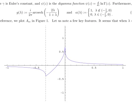
where γ is Euler’s constant, andψ(z) is thedigamma function ψ(z) = _dzd ln Γ(z). Furthermore,

g(λ) := i

2πarcsech −

2λ

1 +λ

!

and α(λ) :=

(

1, λ /_∈(₋1₃,0) 0, λ∈(−1

3,0).

(5.2) For reference, we plot Aee in Figure 1. Let us note a few key features. It seems that when λ = 1,

-1 -0.5 0.5 1

[image:13.612.79.540.74.434.2]

-1 -0.5 0.5 1

Figure 1: Aee as a function of λ. The dashed line is at λ=−1/3.

Aee is not well defined. However, careful analysis will show that in factAee is continuous there and

Aee(λ = 1) =−

3 4V

rr

00 +

7ζ(3) 2π2

where ζ(z) is the celebrated Riemann ζ-function.

Also despite the discontinuity of α(λ), Aee is well-defined at λ = −1/3 =M(k = 0). We can

compute both limits from the left and the right to obtain

Aee(−

1 3) =−

3 4V

rr

00 =−

3 4ln

27

16. (5.3)

This incidentally proves the identity (2.11), which has so far escaped the literature4_{. The reason for}

this good behaviour is that neark = 0, _N(k)_∼1,_hk_|vei ∼k and λ−M(k) =−1/3−M(k)∼k2, 4_{This is due to the fact that from (2.11), we have the expression forA}

ee atλ=−1/3 as

Aee(λ=−

1 3) =

Z +∞ −∞

dk hk|veihve|ki

N(k)(−1/3−M(k))=−3

Z +∞ −∞

dk hk|veihve|ki

N(k)(1 + 3M(k))=−3hve| 1

so the integrand is well defined. This is not true for λ= 0 where Aee diverges as ln ln(λ). In fact

Aee(λ →0)∼

2γ+ 16 ln(2)−9 ln(3)−2 ln(2π) + 2 ln(−ln|λ|) 4

One root ofDet can be found by solving

Aee =−

3 4V

rr

00 +b

1 2(1₋λ) −

3 8

!

≡Ib(λ) (5.4)

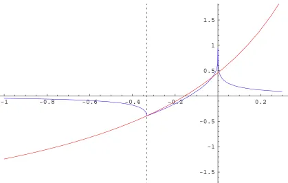
By studying the intersection of Ib(λ) with Aee(λ) we see that there are two kinds of roots (cf.

Figure 2). We note that Ib(λ) is a hyperbola with asymptote at λ = 1 so from −∞ to 1 it is

an increasing function from −3

4β to ∞. Therefore the first kind of root exists no matter what b is (we recall that b > 0), namely they are λ = ₋1/3 (because Ib always passes through the

point (−1/3,−3/4 ln(27/16)) ∼ (−1/3,−0.392436), the left cusp point of Aee; we will show this

below) and some λ1 ∈ (0,1). However when Ib increases fast enough, it could intersect Aee one

more time in the region [₋1/3,0); this is when dIb

dλ|−1/3 ≥ dAee

dλ |−1/3. So the critical point occurs at dIb

dλ|−1/3 = dAee

dλ |−1/3 ⇒b = 8 ln 2. Therefore a second kind of root exists in addition to the first only

when b_≥8 ln 2 and is located in the region [₋1/3,0).

As promised, we will now show that indeedλ=−1/3 =M(k = 0) gives 1−3β(14(−λ−λ)1)−2bAee = 0.

To see this, we recall from (5.3) thatAee(λ=−₃1) =−3₄V00rr. Using this we can calculate

1₋ 4(λ−1)

3β(1₋λ)₋2bAee = 1−

4(−1/3−1) 3(Vrr

00 +b/2)(1 + 1/3)−2b

(₋3 4)V

rr

00 = 0.

We see therefore thatIb(λ) passes through the left cusp of Aee(λ) andλ =−1₃ indeed is a root

of Det.

5.2 The Function Aoo

By the same method we can evaluate

Aoo(λ) :=

Z ∞

−∞

dt t

3 sinh(t)

2 (1 + 2 cosh(t)) (1 +λ+ 2λcosh(t)). Now we obtain

Aoo(λ) =

3

4 2γ+ 3 ln 3 +ψ[1 +g(λ)] +ψ[1−α(λ)−g(λ)]

!

,

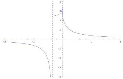
where g(λ) and α(λ) were defined in (5.2). We plot Aoo in Figure 3. There are several important

points here as well. Firstly putting λ = 1 we get hvo|₁₋1_M |voi = 3₄Voorr, giving us the nice identity.

Secondly Aoo diverges at λ= 0 from both sides. The divergence is again very slow, as ln lnλ:

Aoo(λ →0)∼

3 (2γ+ 3 ln(3)₋2 ln(2π))

4 +

-1 -0.8 -0.6 -0.4 -0.2 0.2

[image:15.612.98.517.73.339.2]

-1.5 -1 -0.5 0.5 1 1.5

Figure 2: The intersection of Aee with Ib as functions of λ. We have here chosen a b above the critical

value b0 so that we can explicitly see 3 points of intersection. Note that both Aee and Ib always meet at

least at the dashed line atλ=₋1/3.

More important is the behavior near λ =₋1/3. If we approach from the left we find Aoo|(−1 3)− =

−∞. If we approach from the right, we find Aoo|(−13)+ =

3

4ln 27 which is finite. This discontinuity

may seem unnatural, but we will see later that it is consistent with our analysis. Now we can solve the other λ which makes Detzero. The equation is

Aoo =

3β

4 = 3 4 ln

27 16 +

b

2

!

. (5.5)

From this we find again that there are two kinds of solutions. The first one does not depend on the value ofb and is located in the region (0,1) (since b >0). For large enough b, of course, we obtain a second type of zero in addition to the first, located in the region [−1/3,0). This occurs when the right hand side is higher than when Aoo takes its point of discontinuity at λ =−1/3; this is when

b_≥8 ln 2. Comparing with the critical value ofb found in theAee case, we find they are same. This

is not an accident.

In fact we claim that the solutionsλ found in both cases, either fromAee or fromAoo, whether

in the region (0,1) or [₋1/3,0) are the same, i.e., the two roots of Det are degenerate. To show this, we use the analytic form of Aee and Aoo, giving the ratio

1₋ 4 3βAoo

1_{− 3β(1}4(₋λ−_λ1)_)−2bAee

= b+ 3bλ+ 6(λ−1) ln

27 16

-2 -1 1 2

[image:16.612.96.511.77.344.2]

-4 -3 -2 -1 1 2 3 4

Figure 3: Aoo as a function ofλ. The dashed line is atλ=−1/3.

As analysed, the denominator gives one root ofDetand the numerator, the other. The idea is that if the roots are degenerate, they will cancel each other so that this ratio is neither zero nor infinite at the roots. From (5.6) we see that the ratio is zero only whenλ= (6 ln(27/16)₋b)/(3b+6 ln(27/16)); careful analysis reveals that this zero is coming from the simple pole in the denominator at 3β(1₋

λ)−2b = 0 and so is in fact not a zero of Det. On the other hand, the only pole is at λ =−1/3. We hence conclude that the two zeros of Detare degenerate5 _{except for λ=−}1

3 which is a zero of

the denominator only (for all values ofb).

6. The Discrete Spectrum

Having discussed the continuous spectrum, we now move on to the discrete spectrum. This comes from the zeros of the determinant Det. The solutions have been discussed in section 5. In this section, we will construct the corresponding eigenvectors.

6.1 The Case of λ=₋1/3

As we have shown, no matter what b is, Mee = 1− _3β(14(λ₋−_λ)1)_−2bAee = 0 always has a solution

λ = −1/3. We will denote the corresponding eigenvector as v_+,−1

3. Furthermore, when b ≥ 8 ln 2,

5_{The degeneracy between the zeros ofA}

oo andAee is broken in the limitb= 0. In this case,Det= 0 forAoohas

solution atλ= 1 while there is no solution for Aee in the region (0,1]. However this case ofb= 0 is not a physical

both Mee and Moo = 1−₃4_βAoo have another solution λ ∈[−1/3,0). When b = 8 ln 2, the solution

will be λ=−1/3 again, which is also degenerate6_.

Now we can start to construct the eigenvectors. SinceMee = 0, for consistency of (4.19), we need

Be = 0. This can be achieved by choosing anyk0 6= 0 ork0 = 0 such thatr(k = 0)/(−1₃−M(k = 0))

is not a pole.

If we choose k0 6= 0, we haveBo = 0 and the solution is7

Ce =

2Vrr oo

√

2b, Co = 0 (6.1)

and the eigenvector becomes

g = 1,

Z +∞

−∞ dkh(k)|ki =

Z +∞

−∞ dk − 8 3√2b

|ki hk|vei

N(k)(₋1/3₋M(k))

!

= − 8

3√2b

1

(₋1/3₋M)|vei = √8

2b

1

1 + 3M |vei.

In summary then,

v_+,−1 3 =

"

1

8

√

2b

1 1+3M |vei

#

(6.2) which is the solution given in [12] (equation (4.5)). Notice that this state istwist-even. This solution has been found by several groups already [17, 12, 20].

If instead of choosing k0 6= 0, we choose k0 = 0 such that r(k)/(−1/3−M(k)) does not have

a pole at k = 0, then there are two cases. The first one is that r(k)/(₋1/3₋M(k)) has a zero at k = 0, so we have Bo = 0 and the solution is the same as above. The second one is that

r(k)/(−1/3−M(k))∼1 atk = 0, then we will have a non-zeroBo. We point out that this is when

b ₆=b0 := 8 ln 2. Indeed if b =b0, consistency of (4.19) requires Detand hence Bo to be zero. This

non-zeroBoopens the possibility for another eigenvector. If we choose the branch Aoo|(−1

3)− =−∞,

we will have _Co = 0 althoughBo 6= 0. However, if we choose the branchAoo|(−1 3)+ =

3

4ln 27, we get

a nonzeroCo. In this case we can construct two eigenvectors: one is twist-even and one is twist odd.

Let us work out the details. Setting k0 = 0 and expanding around k = 0 we obtain (−1/3− M(k))_∼k2_+O(k3_{) (the first order is zero). Therefore we can choose the parametre r(k) =k}2 _and

get Bo =−6

√

3/π. Then _Co =− 6

√

3

π(1−ln 27

β )

. If we set _Ce = 0, we get the eigenvector as

v_−,−1 3 =

"

0

4Co 3β

1

−1/3−M |voi −

36

π2 |k = 0i

#

. (6.3)

6_{Notice that the existence of zeros for M}

oo at b = 8 ln 2 depends crucially on the existence of the limit of Aoo

when we reachλ=₋1/3 from the right.

7_{Here in principle we can choose}

Ce to be any non-zero value. What we choose here is just a convenience to

We can check this directly by acting M′ _{on the left. Using}

hve|k = 0i= 0, hve|

1

−1/3₋M |voi= 0, hvo|k= 0i= √

3π

6 , Aoo|(−13)+ =

3 4ln 27. If we choose Ce= 2V

rr oo

√

2b , we will get

v′ =

" 1 8 √ 2b 1

1+3M |vei+

4Co 3β

1

−1/3−M |voi −

36

π2 |k = 0i

#

.

From these two solutions we can construct the twist-odd solutionv_−,−1

3 and the twist-even solution

v_+,−1 3 = v

′_−v −,−1

3, which is equal to (6.3). In fact, comparing with the results (4.29) and (4.30)

from the last section, we find that these two solution v_±,−1

3 are nothing new, but a part of the

continuous spectrum we presented before.

It is a little strange that we get twist-even and twist-odd states for M′ _{at λ = −1/3 at the} same time while for M, we have only a twist-odd state. To see that it is true, let us take b →+∞. In this limit we have from (2.8)

M′ =

" −1 3 0 0 M # .

From this limit, we see immediately thatM′ _{has two eigenvectors for the eigenvalue −}1 3: v+ =

"

1 0

#

, v₋ =

"

0

|k = 0_i

#

; these are of course nothing other than the limit of v_±,−1

3 when b → +∞. We consider this as a

strong evidence supporting the double degeneracy at λ=₋1/3. In the conclusions section, we will give some numerical evidence and further discussion about this point.

We have discussed the case of b 6= b0 in the above and found that the discrete spectrum at λ = ₋1/3 is the same as the continuous at this point. Now we discuss the special case when

b = b0 = 8 ln 2. Recall from Subsection 5.2, we must choose the branch of Aoo|(−1 3)+ =

3

4ln 27 in

order to get a zero for the determinant. Consistency of (4.19) requires Be = Bo = 0. This can be

achieved by setting k0 6= 0 or by setting k0 = 0 but with r(k)/(−1/3−M(k)) having a zero at k = 0. In either choice we will get two eigenvectors by letting _Ce 6= 0, Co = 0 or Ce = 0, Co 6= 0.

The results are

vb0

+,−1 3 = " 1 8 √ 2b 1 1+3M |vei

#

(6.4) and

vb0

−,−1 3 =

"

0

4Co 3β

1

−1/3−M |voi

#

. (6.5)

Notice that althoughvb0

+,−13

is the same as (6.2),vb0

−,−13

is different from (6.3) by missing the _|k = 0_i term. This is a very important point. It in fact distinguishes the continuous and the discrete spectra. This means that when b0 6= 8 ln 2, the continuous spectrum at λ = −1/3 is simply the

discrete spectrum at this point. However whenb0 = 8 ln 2, the expressions (4.29) and (4.30) for the

6.2 Other Solutions at λ6=−1/3

For other λ 6= −1/3 which make Det zero no matter which region they are, the eigenvectors can be found similarly. First we choose _Ce 6= 0, Co = 0 and the eigenvector is twist even

v+ =

1

2(v(k0) +v(−k0)) =





2√2b

3β(1−λ)−2bCe(k0)

4(λ−1)

3β(1−λ)−2bCe(k0)

1

λ−M |vei



. (6.6)

Next we chooseCe = 0, Co 6= 0 and the eigenvector is twist odd

v₋ = 1

2(v(k0)−v(−k0)) =

"

0

4

3βCo(k0)

1

λ−M |voi

#

. (6.7)

Again, when λ ∈ [−1/3,0) the expressions (4.29) and (4.30) for the continuous spectrum will be replaced by these above expressions for the discrete spectrum.

7. The Generating Function

In the above sections, we have given the eigenvectors ofM′ _{for the various ranges ofλ. They are} of the form of_|vei and|voiacted on by _λ−1_M. It would be very nice if we could explicitly determine

these components. The present section solves this problem.

In order to find components, we need to find the generating function. The idea is that, recalling

fk in (2.3) we can define generating functions Ge(z) and Go(z) as follows:

Ge(z)≡ hz|E−1

1

λ₋M |vei =

Z +∞

−∞ dk

fk(z)hk|vei

N(k)(λ₋M(k)), (7.1)

Go(z)≡ hz|E−1

1

λ₋M |voi =

Z +∞

−∞ dk

fk(z)hk|voi

N(k)(λ₋M(k)). (7.2) The series expansion coefficients in z of Ge(z) (respectively Go(z)) will give the components of

1

λ−M |vei (respectively

1

λ−M |voi).

Recalling the definition offk in (2.3), as well as (2.3) and (2.4), in addition to (2.2) and (2.6),

the integrals have the explicit forms

Ge(z) =

Z +∞

−∞ dk

1₋e−karctanz _{−1 + cosh(}k π

2 )

2k 1 + 2 cosh(k π₂ )

λ+ _{1+2 cosh(}1 k π

2 )

sinh(k π₂ )

(7.3)

Go(z) =

Z +∞

−∞ dk

√

3 1₋e−karctanz

2k 1 + 2 cosh(k π₂ )

λ+ _{1+2 cosh(}1 k π

2 )

(7.4)

7.1 The Twist-even States

For the generating function Ge(z), when λ ∈ [−1/3,0), setting λ = −(2 cosh(πk₂0) + 1)−1 we

have8 Ge(z) =

1 + 2 cosh(πk0

2 )

4k0(1 + cosh(πk₂0))

k0B[e−4iarctanz; 1− ik0

4 ,0] +k0B[e

−4iarctanz_{; 1 +} ik0

4 ,0] +k0(2γ−4arctanh(e−2iarctanz) + ln(16) +ψ(−

ik0

4 ) +ψ(

ik0

4 ))−4isinh(k0arctanz)

!

(7.5) where

B[z;a, b]≡Bz[a, b] = z

Z

0

ta−1(1−t)b−1dt

for (Re(a)>0) is theincomplete beta function. Forλ1 ∈(0,1) we set

λ1 = (2 cosh( πk0

2 )−1)

−1 _(7.6)

and have

Ge(z) =

i(₋1 + 2 cosh(πk0

2 ))csch 2₍πk0

4 )

2 iarctanh(e

−2iarctanz₎

−i

4 2γ+ ln(16) +ψ( 1 2−

ik0

4 ) +ψ( 1 2+

ik0

4 )

!

+e−

(k0+2i) arctanz

2i+k0

2F1[

1 2−

ik0

4 ,1, 3 2 −

ik0

4 , e

−4iarctanz_]

+e

(k0−2i) arctanz

2i₋k0 2 F1[

1 2+

ik0

4 ,1, 3 2+

ik0

4 , e

−4iarctanz_]

!

(7.7) where

2F1[a, b, c, z] =

Γ(c) Γ(b)Γ(c−b)

1 Z

0

tb−1(1−t)c−b−1(1−tz)−adt

(for Re(c)>Re(b)>0;_|Arg(1₋z)_{| ≤}π) is the hypergeometric functionof the first kind.

As an application of the above generating function, we derive the components of the state

v_+,−1

3 in (6.3). Taking the limit λ→ −1/3 (or equivalently k0 →0) we can simplify the generating

function Ge(z) as

Ge(z)|k0=0 =

3

4ln(1 +z

2_{) (7.8)}

= ₋3 4

X

n≥1

(₋)n

n z

2n₌₋3

2

X

k=even

1

√ k

(₋)k/2 √

k z

k_{. (7.9)}

8_{All ensuing results will be correct only for}

|z_|< π

4 because of a choice of branch cut; this is no hindrance because

We conclude therefore that (up to an overall factor) the twist-even eigenvector at λ =−1/3 (from (6.2)) has components

vk=

4

√

2b

(−1)k/2 √

k k even and >0,

v0 = 1 andvk = 0 for k odd. This reproduces the result given in equation (4.15) of [17] for9 b= 4. 7.2 The Twist-odd States

Now we discuss the generating function Go(z). Again, when λ ∈ [−1/3,0) we can set λ =

−1/(2 cosh(πk0/2) + 1) and obtain Go(z) =

√

3(2 coth(πk0

2 ) + csch(

πk0

2 ))

4 B[e

−4iarctanz_{; 1}

− ik₄0,0]₋B[e−4iarctanz; 1 + ik0 4 ,0] +4icosh(k0arctanz)

k0 −

iπcoth(πk0 4 )

!

. (7.10)

On the other hand, when λ1 ∈(0,1) we can set λ1 = 1/(2 cosh(πk0/2)−1) and obtain Go(z) =

i√3(−1 + 2 cosh(πk0

2 ))csch(

k0π

2 )

8k0 −

i(k0−2i)B[e−4ia,

1 2−

ik0

4 ,0] +e−2(4i+k0)a 4e

(6i+k0)a₍−_2i+k

0+ 2e2k0ak0)

k0−2i 2

F1[1,

1 2 + ik0 4 , 3 2+ ik0

4 , e −4ia_]

−2e(k0+2i)a 8i

k0+ 6i 2 F1[2,

3 2 − ik0 4 , 5 2 − ik0

4 , e −4ia_]

+ 8i

k0−6i 2 F1[2,

3 2 + ik0 4 , 5 2+ ik0

4 , e −4ia

] +e(k0+6i)a_k

0πtanh( k0π

4 )

!!!

, (7.11) where a≡arctanz.

As an application, we now try to find the components ofv_−,−1

3. This is the twist-odd eigenvector

at eigenvalue λ = ₋1/3 whose existence is so-far unpredicted. As we have mentioned, this state exists only when we reach λ =₋1/3 from the right hand side. This corresponding to k0 → 0 and

we find the limit

Go(z)|₋(1 3)+ =

i√3

8π [24(arctanz)

2_−π2_{+ 6 ln(e}−4iarctanz_{) ln(1−e}−4iarctanz_{) + 6Li}

2[e−4iarctanz]]

= 3

√

3z

π −

7z3 √

3π +

43√3z5

25π −

337√3z7

245π +

1091z9

315√3π +... (7.12)

where Li2[z] =

∞

P

k=1z

k_/k2 _{(for |z|<1) is the dilogarithm function.}

9_{We think that Equation (4.2) (and therefore (4.15)) of [17] is compatible withb= 4, as can be checked by solving}

these equations for U′

8. The spectrum of

M

′12

and

M

′21

We digress here for a moment to present another application of our analysis. Knowing the spectrum of M′₁₁

≡M′ _{it is easy to calculate that of the matrices M}′12 _{and M′}21_.

The method is in direct parallel to the discussions in [9] because the matrices M′rs

obey the same useful properties as the matrices Mrs_:

[M′rs

, M′r′_s′

] = 0 _∀r, s, r′_{, s}′ _{= 1,2,3 (8.1)}

M′ +M′12+M′21 = (M′)2+ (M′12)2+ (M′21)2 = 1 , M′12M′21=M′(M′−1). (8.2) From (8.1), we see that allM′rs

share the same eigenvectors. The continuous eigenvaluesλ12_(k)

and λ21_{(k) of M}′12

and M′21

respectively, can then be calculated by treating (8.2) as a system of equations in λrs_{(k). We thus obtain:}

λ12(k)−λ21(k) = ±q(1−λ(k))(1 + 3λ(k)) (8.3)

λ12(k) +λ21(k) = 1₋λ(k). (8.4) Because in the limit b _{→ ∞}, M′12

and M′21

have similar diagonalized form as M′_{, we should} obtain the same eigenvalues as for the matrices Mrs_{. We can extend the choice of sign in front of}

the square root (from [9])10 _{to finite values of b. We therefore have, for the continuous spectrum,} λ12(k) = 1

2sign(k)

q

(1₋λ(k))(1 + 3λ(k)) + 1

2(1−λ(k)) (8.5)

λ21(k) = ₋1

2sign(k)

q

(1₋λ(k))(1 + 3λ(k)) + 1

2(1−λ(k)). (8.6) Furthermore the doubly degenerate eigenvalue λ1 of M′ gives rise to the following 2 eigenvalues:

λ12₁₊ =λ21_{1+ ≡}λ1+ =

1 2

q

(1₋λ1)(1 + 3λ1) +

1

2(1−λ1) (8.7)

λ12₁₋=λ21₁₋≡λ1− = − 1 2

q

(1−λ1)(1 + 3λ1) +

1

2(1−λ1). (8.8) Because λ1 ∈(0,1), we have that λ1+ ∈(0,1) and λ1− ∈

−1 3,0

.

9. Discussions and Conclusions

In this paper, we solved the eigenvalue and eigenvector problem for the matrix M′_{. We found} that its spectrum is composed of a continuous spectrum, which is the same as the spectrum of

M, and a new discrete spectrum, which always contains an eigenvalue λ1 in the range (0,1). We

obtained the closed form for all the eigenvectors and found that, for every eigenvalue (including

−13), we have always one twist-even state and one twist-odd state.

A particular thing that we found is that there is a critical valueb0 = 8 ln 2 above which one pair

of eigenvectors in the continuous spectrum is replaced by one pair of eigenvectors in the discrete spectrum, although the eigenvalue does not change. As the parameter b is claimed to be irrelevant to the physics[2, 23], it would be interesting to understand the meaning of this critical value b0.

The main difference between the spectrum ofM′ _{and that ofM is that the eigenvalue−}1

3 is now

doubly degenerate, and that we have one new doubly degenerate eigenvalue in the interval (0,1). As we mentioned in Section 6, the double degeneracy at λ = −1

3 is a little mysterious although

we have several pieces of evidence to support it. This degeneracy is a surprising result of our analysis. Indeed, in the light of [26, 20] it seems to mean that we now would have two commuting coordinates in the Moyal product decomposition of the star product. It is thus worth looking closer at our twist-odd eigenvector v_−,−1

3.

Let us try to see if level truncation can help us decide ifv_−,−1

3 really is an eigenvector. For this

we define w(b, L) = ₋3M′_v −,−1

3(b), where M

′ _{and v} −,−1

3 are truncated to level L. If v−,− 1 3 is an

eigenvector of M′ _{with eigenvalue −}1

3, we expect that w(b, L→ ∞) = v−,−13(b) for any value of b.

We show in the following table, the five first nonzero components of w(b = 1) at various levels of truncation, as well as their values extrapolated from a fit of the forma0+a1/log(L) +a2/log(L)2+ a3/log(L)3. In the last lines, we show their exact values as calculated from (7.12).

L w(b = 1)1 w(b= 1)3 w(b = 1)5 w(b= 1)7 w(b = 1)9

100 0.119343 0.41301 -0.446308 0.43575 -0.416943 150 0.120588 0.447491 -0.487193 0.479292 -0.461839 200 0.121053 0.468778 -0.512582 0.506505 -0.490075 300 0.121347 0.49465 -0.543575 0.539889 -0.524878 400 0.121394 0.510341 -0.562439 0.560288 -0.546226

∞ 0.0984355 0.799035 -0.921314 0.962239 -0.980627 exact value 0.119946 0.608215 -0.681026 0.689616 -0.682686

Comparing the two last lines, we see that the result of the fit is about 20 to 40% away from the exact value. Though discouraging, this discrepancy is not conclusive because the fitting function might not be a judicious choice. Indeed note that the convergence is monotonic and very slow, and the values of the fit are surprisingly far away from our finite level values.

For comparison, we show in the next table w+(b, L) = −3M′v+,−1

3(b) for b = 1 in the level

truncation.

L w+(b = 1)0 w+(b= 1)2 w+(b= 1)4 w+(b = 1)6 w+(b = 1)8

100 0.874064 -1.86078 1.27486 -1.01287 0.855905 150 0.903461 -1.89268 1.30621 -1.04427 0.887334 200 0.920118 -1.91092 1.32429 -1.06252 0.905733 300 0.938883 -1.9316 1.34494 -1.08348 0.926978 400 0.949481 -1.94335 1.35673 -1.0955 0.939219

∞ 1.02072 -2.03708 1.46506 -1.2184 1.07553

We see that it converges towards the expected value much better than the C-odd vector does. We can try to compare this difference in numerical behavior to the case of the matrix M. Remember that in [9], the authors found a candidate C-even eigenvector (denoted v+_{) of eigenvalue −}1

3, in

addition to the C-odd eigenvector v−_{. This candidate was however discarded by the authors for} several reasons:

• v+ _{is an eigenvector of K}2

1 but not ofK1.

• The set of eigenvectors without v+ _{already forms a complete basis [10].} • The norm of v+ _{has a worse divergence than the norm of v}−_.

• v+ _{never appears in the level truncation.}

Our analysis does not allow us to generalize these two first arguments to our case11_{. But we can}

do the same level truncation tests as above with the vectors v+ _{and v}−_{. In the following table, we} show u+_{≡ −3Mv}+ _{at various truncations levels as well as the expected values.}

L (u+₎

2 (u+)4 (u+)6 (u+)8 (u+)10

100 1.12259 -1.00375 0.90241 -0.822676 0.758504 150 1.1771 -1.06413 0.965334 -0.886898 0.823385 200 1.21013 -1.10103 1.00408 -0.926709 0.863861 300 1.24965 -1.14547 1.051 -0.975174 0.913374 400 1.27328 -1.17218 1.07933 -1.00457 0.943521

∞ 1.65594 -1.63066 1.58908 -1.55458 1.46357

v+ _{1.41421 -1.33333 1.25196 -1.18525 1.13039}

Now we compare this to the same analysis done with u− _{≡ −3Mv}−_.

L (u−₎

1 (u−)3 (u−)5 (u−)7 (u−)9

100 0.957182 -0.531943 0.399565 -0.328769 0.283024 150 0.967172 -0.542301 0.410247 -0.33963 0.293974 200 0.97283 -0.548233 0.416417 -0.345949 0.300388 300 0.979205 -0.554972 0.423469 -0.353213 0.307799 400 0.982806 -0.558804 0.4275 -0.357384 0.312072

∞ 1.00694 -0.590333 0.46527 -0.400556 0.360073

v− _{1 -0.57735 0.447214 -0.377964 0.333333} We see that the difference in numerical behavior betweenv_−,−1

3 andv+,− 1

3 is qualitatively similar to

the difference in numerical behavior betweenv+_andv−_{. This suggests that we should be suspicious}

11_{In principle, it should be possible to check the completeness, but until now we haven’t been able to simplify the}

about v_−,−1

3. The eigenstate indeed deserves further investigation. However, as we have shown in

the limit b_{→ ∞}, we do believe the existence of the state v_−,−1

3. We think that the reason why the

level truncation does not work is that the components of v_−,−1

3 do not decay fast enough and level

truncation is not very trustable in this case.

Let us move onto the other eigenvalues. The existence of the discrete eigenvalueλ1 in the range

(0,1) can be considered as the result of us adding zero modes into the matrix M to get M′_{. This} relationship may help us to understand the physical meaning of these discrete states. As a check, we can calculate the eigenvalues numerically in the level truncation scheme. We found that the eigenvalue in region (0,1) converges very fast as the level is increased; this situation is very different from that for λ =−1

3 for example, which converges only logarithmically in level truncation [2, 9].

To illustrate this, we write in the following table the value of λ1 atb= 0.2,b = 1 andb= 5, found

at various levels of truncation, as well as its exact values calculated from (5.4).

level 1 5 10 50 100 exact value

λ1(b = 0.2) 0.78606702 0.80099138 0.80260995 0.80326016 0.80328899 0.80329559 λ1(b= 1) 0.39394374 0.40376417 0.40407525 0.40411239 0.40412026 0.40412740 λ1(b= 5) 0.01082671 0.02795012 0.02859612 0.02873404 0.02873526 0.02873810

We see that, at level 10, the relative error is less than 1%. And for b = 0.2 and b = 1, level 1 is already a good approximation.

We hope that the results of this paper can find useful applications. In particular they should lead to some information about the instantonic sliver [18, 19]. Some future work could consist of seeking a better understanding of the density of eigenvalues in the continuous spectrum. Indeed, we have found no convincing argument to claim that it should be the same as for the matrix M. In fact, if those densities were the same, we could simplify the continuous spectrum between the numerator and the denominator of the ratio

R = Tp

2π√α′_Tp+1 =

3Vrr

00 +2b 2

√

2πb3

det(1₋M′₎3

4(1 + 3M′) 1 4

det(1₋M)34(1 + 3M) 1 4

.

But this would lead to a puzzle because M′ _{has two eigenvectors with eigenvalue −}1

3 (at least we

Acknowledgements

We would like to extend our sincere gratitude to Professor Barton Zwiebach for suggesting this project to us and for many insightful discussions and comments. We would also like to thank Ian Ellwood for stimulating conversation, and Professor Wati Taylor for discussion of [17]. We gratefully acknowledge Dmitri Belov for very useful conversations and suggestions to the first draft. This Research was supported in part by the CTP and LNS of MIT and the U.S. Department of Energy under cooperative research agreement # DE-FC02-94ER40818. N. M. and Y.-H. H. are also supported by the Presidential Fellowship of MIT.

References

[1] L. Rastelli, A. Sen and B. Zwiebach, “String field theory around the tachyon vacuum,” arXiv:hep-th/0012251.

[2] L. Rastelli, A. Sen and B. Zwiebach, “Classical solutions in string field theory around the tachyon vacuum,” arXiv:hep-th/0102112.

[3] L. Rastelli, A. Sen and B. Zwiebach, “Half strings, projectors, and multiple D-branes in vacuum string field theory,” JHEP 0111, 035 (2001) [arXiv:hep-th/0105058].

[4] L. Rastelli, A. Sen and B. Zwiebach, “Boundary CFT construction of D-branes in vacuum string field theory,” JHEP0111, 045 (2001) [arXiv:hep-th/0105168].

[5] L. Rastelli, A. Sen and B. Zwiebach, “Vacuum string field theory,” arXiv:hep-th/0106010.

[6] D. Gaiotto, L. Rastelli, A. Sen and B. Zwiebach, “Ghost structure and closed strings in vacuum string field theory,” arXiv:hep-th/0111129.

[7] L. Rastelli, A. Sen and B. Zwiebach, “A note on a proposal for the tachyon state in vacuum string field theory,” arXiv:hep-th/0111153.

[8] E. Witten, “Noncommutative Geometry And String Field Theory,” Nucl. Phys. B268, 253 (1986).

[9] L. Rastelli, A. Sen and B. Zwiebach, “Star algebra spectroscopy,” arXiv:hep-th/0111281.

[10] K. Okuyama, “Ghost kinetic operator of vacuum string field theory,” JHEP 0201, 027 (2002) [arXiv:hep-th/0201015].

[11] H. Hata and T. Kawano, “Open string states around a classical solution in vacuum string field theory,” JHEP 0111, 038 (2001) [arXiv:hep-th/0108150].

[12] K. Okuyama, “Ratio of tensions from vacuum string field theory,” arXiv:hep-th/0201136.

[13] T. Okuda, “The equality of solutions in vacuum string field theory,” arXiv:hep-th/0201149.

[15] V. A. Kostelecky and R. Potting, “Analytical construction of a nonperturbative vacuum for the open bosonic string,” Phys. Rev. D 63, 046007 (2001) [arXiv:hep-th/0008252].

[16] K. Furuuchi and K. Okuyama, “Comma vertex and string field algebra,” JHEP 0109, 035 (2001) [arXiv:hep-th/0107101].

[17] G. Moore and W. Taylor, “The singular geometry of the sliver,” JHEP 0201, 004 (2002) [arXiv:hep-th/0111069].

[18] D. J. Gross and W. Taylor, “Split string field theory. I,” JHEP 0108, 009 (2001) [arXiv:hep-th/0105059].

[19] D. J. Gross and W. Taylor, “Split string field theory. II,” JHEP 0108, 010 (2001) [arXiv:hep-th/0106036].

[20] Private communications with B. Zwiebach; also L. Rastelli, A. Sen, and B. Zwiebach, unpublished.

[21] D. J. Gross and A. Jevicki, “Operator Formulation Of Interacting String Field Theory,” Nucl. Phys. B283, 1 (1987).

[22] D. J. Gross and A. Jevicki, “Operator Formulation Of Interacting String Field Theory. 2,” Nucl. Phys. B287, 225 (1987).

[23] P. Mukhopadhyay, “Oscillator representation of the BCFT construction of D-branes in vacuum string field theory,” JHEP 0112, 025 (2001) [arXiv:hep-th/0110136].

[24] L. Bonora, D. Mamone and M. Salizzoni, “B field and squeezed states in vacuum string field theory,” arXiv:hep-th/0201060.

[25] B. Feng, Y.-H. He and N. Moeller, to appear soon.