City, University of London Institutional Repository
Citation
:
Giraitis, L., Kapetanios, G. and Price, S. (2013). Adaptive forecasting in the presence of recent and ongoing structural change. Journal of Econometrics, doi:10.1016/j.jeconom.2013.04.003
This is the unspecified version of the paper.
This version of the publication may differ from the final published
version.
Permanent repository link:
http://openaccess.city.ac.uk/2400/Link to published version
:
http://dx.doi.org/10.1016/j.jeconom.2013.04.003Copyright and reuse:
City Research Online aims to make research
outputs of City, University of London available to a wider audience.
Copyright and Moral Rights remain with the author(s) and/or copyright
holders. URLs from City Research Online may be freely distributed and
linked to.
Adaptive forecasting in the presence of recent and ongoing
structural change
Liudas Giraitis
Queen Mary, University of London
George Kapetanios
∗Queen Mary, University of London
Simon Price
Bank of England and City University, London.
January 23, 2013
Abstract
We consider time series forecasting in the presence of ongoing structural change where both the time series dependence and the nature of the structural change are unknown. Meth-ods that downweight older data, such as rolling regressions, forecast averaging over different windows and exponentially weighted moving averages, known to be robust to historical struc-tural change, are found also to be useful in the presence of ongoing strucstruc-tural change in the forecast period. A crucial issue is how to select the degree of downweighting, usually defined by an arbitrary tuning parameter. We make this choice data-dependent by minimising fore-cast mean square error, and provide a detailed theoretical analysis of our proposal. Monte Carlo results illustrate the methods. We examine their performance on 97 US macro series. Forecasts using data-based tuning of the data discount rate are shown to perform well.
Key words: recent and ongoing structural change, forecast combination, robust forecasts.
JELClassifications: C100, C590.
1
Introduction
It is widely accepted that structural change is a crucial issue in econometrics and forecasting. Clements and Hendry suggest forcefully (in e.g. 1998a,b) that such change is the main source of forecast error; Hendry (2000) argues that the dominant cause of forecast failures is the presence of deterministic shifts. Convincing evidence of structural change was offered by Stock and Watson (1996) who looked at many forecasting models of a large number of US time series, and found parameter instability in a substantial proportion. This issue remains relevant: in a survey of the literature on forecasting in the presence of instabilities for theHandbook of Forecasting, Rossi
∗The views expressed are those of the authors, and not necessarily those of the Bank of England or Monetary
(2012) writes ‘the widespread presence of forecast breakdowns suggests the need for improving ways to select good forecasting models in-sample.’ Our work on robust and data driven forecasting is a contribution to precisely this end. As model parameters may change continuously, drift smoothly over time or change at discrete points in an unknown manner, and both within the sample and over the forecast period, we consider a general setting where the model structure and presence and type of structural change are all unknown.
There is a large literature on the identification of breaks, and forecasting methods robust to them (Rossi (2012)). However, the deeply practical need to forecast after a recent structural change, or during a period of such change, has received very little attention. As most forecast approaches are only effective in specific cases, the problem is compounded by the unknown and therefore unspecified nature of any structural change.
Detection of structural change has a long history, mainly in the context of structural breaks (although see Kapetanios (2007) for the case of smooth structural change). Seminal papers in-clude Chow (1960), Andrews (1993) and Bai and Perron (1998). But the question of amendment of forecasting strategies then arises. While this has been tackled by many authors, a major con-tribution was made by Pesaran and Timmermann (2007). They concluded that, in the presence of breaks, forecast pooling using a variety of estimation windows provides a reasonably good and robust forecasting performance.
Nevertheless, most work on forecasting assumes that change has occurred when sufficient time has elapsed for post-break estimation.1 In practice, the issue of change occurring in real time is a major consideration, which was partly addressed in Eklund, Kapetanios, and Price (2010). They considered a variety of forecasting strategies which can be divided into two distinct groups. In one case the forecaster monitors for change and adjusts methods once change has been detected. In the other the forecaster does not attempt to identify breaks, since that involves a substantial time lag. Instead break-robust forecasting strategies are used that essentially downweight data from older periods deemed to be irrelevant for the current conjuncture.
While moving in an interesting direction, Eklund, Kapetanios, and Price (2010) do not elabo-rate two issues: how much to downweight past data, and whether to do so monotonically. Clearly, any arbitrary discount factor is unlikely to be optimal. And neither may monotonicity: for ex-ample, if regimes (e.g., monetary policy) come and go then older data, from a period where the current regime previously held, might be more relevant than more recent data from other regimes. In this paper, we suggest forecasting approaches that address these issues. Our main contribu-tion is to introduce and analyse a cross-validacontribu-tion based method which selects a tuning parameter defining the downweighting rate of the older data. We show that the implied discount rate min-imises the mean square error (MSE) of the forecast in the weighting schemes considered. Further, we consider a nonparametric method for determining a flexible weighting scheme. The latter does not assume any particular shape for the weight function, nor monotonicity. We explore the
prop-1Exceptions include the interesting work of Clements and Hendry (2006) and Castle, Fawcett, and Hendry
erties of the new forecasting methods for a variety of models in terms of theory, with a Monte Carlo exercise and empirically. It turns out that the method is valid under a wide range of forms of structural breaks and persistence, and can be generalised in a number of practically important dimensions, most notably allowing varying dynamic structures.
A byproduct of our results is a new way to accommodate trends of a generic nature in fore-casting. Unlike many forecasting approaches that require the removal of stochastic or other trends before forecasting, our methods can be directly applied to the level of the forecast series.
The rest of the paper is organised as follows. Section 2 presents our approach for forecasting in the presence of recent structural breaks. We provide its theoretical justification and asymptotic MSE, and describe some robust forecasting strategies. Section 3 includes an extensive Monte Carlo study in which these strategies are evaluated. In Section 4 the methods are used to forecast a large number of US macroeconomic time series, where we find results broadly consistent with the Monte Carlo study. Section 5 concludes. Proofs are reported in an Appendix.
2
Adaptive forecasting: econometric framework
2.1
Forecasting strategies
In this section we work with a simple location forecasting framework that is as general as possible while consistent with clear theoretical results. It may be summarised as
yt=βt+ut, t= 1,· · ·, T, (2.1)
where βt is an unobserved persistent process, and ut is a stationary dependent noise that is
independent of βt. Unlike most previous work we wish to place as little structure as possible
on the process βt. We do not specify whether βt is stochastic or deterministic, or whether it is
discontinuous or smooth. The noise process ut is a stationary linear process with mean zero and
finite variance σu2. The persistent component βt ≡ βT ,t is allowed to be a triangular array, and
can be a stochastic (unit root) or deterministic (bounded) trend. This set-up provides sufficient flexibility to our theoretical analysis of forecastingyt, allowing forβT,tsuch as those used in locally
stationary models (e.g. Dahlhaus (1996)), or in persistent stochastic unit root trend models. For simplicity of notation, we write yT,t as yt and βT ,t as βt. It should be stressed that in robust
forecasting, which is our focus, the structure ofβtis neither known nor estimated. Concerning our
simple location conditional mean modelling, we note that our analysis can allow both the use of a generic model of the conditional mean of the process and robust forecasting around that model. We discuss details related to this extension in Section 2.8.
Eklund, Kapetanios, and Price (2010) find that simple forecasting of yt, based on weighting
weakness is that it is not clear how to select the tuning parameters. So data-dependent tuning methods for choosing these parameters are of great interest.
One way to calibrate parameters is by optimising on in-sample forecasting performance. This idea is not new. For example, Kapetanios, Labhard, and Price (2006) suggest forecasts where different models are averaged with weights that depend on the forecasting performance of each model in the recent past. In what follows we formalise the above ideas, presenting a data-driven weighting strategy and developing its theoretical analysis.
We consider a linear forecast of yt, based on (local) averaging of past values yt−1,· · · , y1:
ˆ
yt|t−1, H = t−1
X
j=1
wtj,Hyt−j =wt1,Hyt−1+· · ·+wt,t−1,Hy1, (2.2)
with weights wtj,H ≥ 0 such that wt1,H +· · ·+wt,t−1,H = 1, parameterised by a single tuning
parameter H. The latter defines the rate of downweighting the past observations (e.g., the width of the rolling window). The structure of weights wtj,H is described in Assumption 1. We assume
that H takes values in the intervalIT = [α, Hmax], where α >0.
Assumption 1 The function K(x) ≥ 0, x ≥ 0 is continuous and differentiable on its support, such that R∞
0 K(u)du= 1, K(0) >0, and for some C >0, c >0
K(x)≤Cexp(−c|x|), |K˙(x)| ≤C/(1 +x2), x >0, (2.3)
where K˙ is the first derivative of K. For t≥1, H ∈IT, set kj,H =K(j/H) and define
wtj,H =
kj,H
Pt−1
s=1ks,H
, j = 1,· · · , t−1. (2.4)
Example 1 The main classes of commonly employed weights satisfy this assumption. (i)Rolling window weights, withK(u) = I(0≤u≤1).
(ii) Exponential weighted moving average (EWMA) weights, with K(u) =e−u, u ∈[0,∞). Then, with ρ= exp(−1/H),kj,H =ρj and wtj,H =ρj/Pt
−1
k=1ρ
k, 1≤j ≤t−1.
(iii) Triangular window weights, withK(u) = 2(1−u)I(0≤u≤1).
While the rolling window simply averages the H previous observations, the EWMA forecast uses all observations y1,· · · , yt−1, increasingly downweighting the more distant past. In practice,
fore-casting of a unit root or trending process yt is often conducted by averaging over the last few
observations. When persistence in yt falls, wider windows may be expected to yield smaller
fore-cast MSE. It is also plausible that for a stationary process {yt} when dependence is sufficiently
strong a forecast discounting past data will outperform the sample mean forecast (yt+· · ·+y1)/t.
These observations, supported by the theory below, indicate that the ‘optimal’ selection of H
depends on the unknown type of persistence in yt. Thus, contrary to the usual practice of using
2.2
Selection of the tuning parameter
H
Given a sampley1,· · · , yT, computation of the forecastyT+1|T , H requires selection of the parameter
H. We use a cross-validation method, obtaining H by numerically minimising the mean squared forecast error of the in-sample forecasts, defined by the following objective function:
QT ,H :=
1
Tn T
X
t=T0
(yt−yˆt|t−1, H)2, Hˆ := argminH∈ITQT ,H (2.5)
with starting point T0 = o(T), Tn :=T −T0+ 1. Define Hmax =T0T−δ, 0 < δ < 1. We assume
that T0 and Hmax are selected such thatT2/3 < Hmax< T0 =o(T).
We will show that the forecast ˆyT+1|T , H ofyT+1, obtained with data-tuned weights (or ˆH),
min-imises the Mean Squared Error (MSE),ωT ,H :=E(yT+1−yˆT+1|T , H)2 inH, hence making the
fore-cast procedure (2.2) operational and optimal in the following sense. Let Hopt = argminH∈ITωT ,H
be the optimal value of fixed parameter H minimising MSEωT ,H. Then
ωT,Hˆ =ωT ,Hopt+o(1), QT ,Hˆ =ωT,Hˆ +op(1), (2.6)
where the quantity QT,Hˆ is an estimate of the forecast error ωT,Hˆ.
Below we verify that the minimisation procedure (2.5) provides optimal selection ofHfor basic forms of persistence in yt = βt+ut. As an illustration, let ˆσT,u2 := Tn−1
PT
j=T0u
2
j be the sample
variance of ut. We will show that, as T → ∞,
QT,H = ˆσT ,u2 +E[QT ,H −σ2u](1 +oP(1)),
= ˆσT ,u2 + (λβH
m
Tp +
λu
H)(1 +oP(1)), H → ∞, (2.7)
with some constants λβ ≥0, λu, and integers m, p≥ 0. The termλβHm/Tp is contributed by βt
while λu/H byut. These relations determine whether ˆH takes finite values or is increasing with
T.
For example, if the noise ut in yt = βt +ut is sufficiently strongly dependent, then using
exponential weights yields λu <0. Then, no matter what βt is, QT ,H reaches its minimum on a
bounded interval, and the minimiser ˆHof (2.7) remains bounded. Similarly, ifytincludes a linear or
unit root trendβt, thenHm/Tp ≥H, and the minimiser ˆHof (2.7) again remains bounded. Under
mildly persistent βt, the minimiser ˆH can also increase as a power of T. For example, if βt is a
bounded unit root trend, andutis an i.i.d. noise, thenQT ,H = ˆσT,u2 +(λβHT−1+λuH−1)(1+oP(1)),
λu >0, which leads to ˆH ∼cT1/2 (see Sections 2.5-2.6). Similar properties hold for the break in
the mean model (see Section 2.6).
Notation. Beside wtj,h, we will use the weights
wj,H =kj,H/
∞
X
s=1
Below, a∧b = min(a, b), a∨b = max(a, b) and I(A) is the indicator function; aT ∼ bT denotes
thataT/bT →1, as T increases. We writeop,H(1) oroH(1) to indicate, that supH∈IT |op,H(1)| →p 0
or supH∈I
T |oH(1)| →0, as T → ∞.
We will use the fact
ˆ
σT ,u2 =σu2+Op(T−1/2), (2.9)
which holds under Assumption 2 (see Proposition 4.5.2 in Giraitis, Koul, and Surgailis (2012)).
2.3
Properties of a forecast based on
H
ˆ
Now we turn to the theoretical justification of the optimal properties of the selection procedure of H for yt = βt + ut, where βt is a persistent process (deterministic or stochastic trend) of
unknown type, and ut is a stationary noise term. Our objective is to show that the forecast
yT+1|T ,Hˆ of yT+1 with optimal tuning parameter ˆH minimises the forecast MSE in the following
sense: ωT ,Hˆ =ωT ,Hopt+oP(1). Moreover, the property QT ,Hˆ =ωT ,Hˆ +op(1) allows estimation of
the forecast error.
The following assumption specifies the required properties of the stationary noise process ut.
Assumption 2 ut is a stationary linear process
ut =
∞
X
j=0
ajεt−j, t∈Z, εj ∼IID(0, σ2ε), Eε41 <∞, (2.10)
such that P
k∈Z|γu(k)|<∞, Pk≥n|γu(k)|=o(log
−2
n) and s2u :=P
k∈Zγu(k)>0, where γu(k) =
Cov(uk, u0).
Under Assumption 2, ut has short memory, while its long-run variance s2u is positive and finite.
We will write ut ∼ I(0) to denote that a stationary process ut satisfies Assumption 2. Below
βt∼I(1) denotes a unit root process such that βt−βt−1 is an I(0) process.
We shall consider the following types of persistent component βt.
b1. Constant βt=µ.
b2. Unit root βt∼I(1).
b3. Bounded unit root T1/2β
t ∼I(1).
b4. Deterministic trend βt=tg(t/T).
b5. Bounded deterministic trend βt=g(t/T).
b6. Break in the mean βt=
µ1, t = 1,· · · , t0,
µ2, t=t0+ 1,· · · , T.
We suppose that, in (b4) and (b5), g(x), x ∈ (0,1) is continuous and has a bounded second derivative, and in (b6), µ1 6=µ2 and τ :=T −t0 =o(T).
2.4
The case of a stationary process
y
tFirst we discuss the properties of the forecast in the case (b1) when yt = µ+ut, t ≥ 1 is a
stationary process. We shall use the following notation: κ2 =
R∞
0 K
2(x)dx, κ
0 =K(0), and
qu,H :=E u0−
∞
X
j=1
wj,Hu−j
2
−σ2u, λu :=s2u{κ2−κ0}+σ2uκ0. (2.11)
Theorem 1 Suppose that yt=µ+ut, t≥1, where ut is a stationary I(0) process.
Then, as T → ∞, for H ∈IT,
QT,H = ˆσ2T,u+qu,H +op,H(H−1), ωT ,H =σu2+qu,H +oH(H−1), (2.12)
where qu,H =λuH−1+o(H−1), as H → ∞.
Theorem 1 shows that QT ,H is a consistent estimate of ωT ,H, and implies that the forecast
yT+1|T ,Hˆ computed with the data-tuned ˆH has the same MSE as yT+1|T , Hopt. The latter can be
estimated byQT ,Hˆ as stated in the following corollary.
Corollary 1 If qu,H reaches its minimum at some finite H0, then
ωT ,Hˆ =ωT ,Hopt+op(1), QT,Hˆ =ωT ,Hˆ +o(1) =σ 2
u+qu,H0 +op(1). (2.13)
If qu,H reaches its minimum at infinity, then
ωT,Hˆ =ωT ,Hopt+o(T
−1/2), Q
T ,Hˆ =ωT ,Hˆ +Op(T−1/2) =σu2+Op(T−1/2). (2.14)
Remark 1 Result (2.13) implies that the forecast with tuning parameter ˆHhas the same precision as the forecast based on Hopt that minimises the forecast error ωT ,H. The sign of λu carries
information about the location of the minimiser ˆH ofQT ,H: for λu <0,QT ,H reaches its minimum
at some finite value H0. In such a case, the error ωT ,Hˆ = σu2 +qu,H0 of the optimal forecast is
smaller than that of the sample mean,σ2
u. The sign of λu is determined by two factors: the kernel
K and the strength of dependence in ut. For the rolling window kernel K(u) = I(0 ≤ u ≤ 1),
κ2 =κ0 = 1, and thusλu =σu2 is always positive. However, for the exponential kernelK(u) =e
−u,
u ≥ 0, λu = σu2 −s2u/2 which becomes negative when the long-run variance of ut is sufficiently
large: s2u > 2σu2, e.g., for an AR(1) model ut with autoregressive parameter greater than 1/3.
The fact thatλu is smaller for exponential weights than for rolling windows suggests that EWMA
weighting leads to a smaller forecast error and may outperform the latter.
Ifqu,H is a positive function, then ˆH will take the largest possible value inIT, and the forecast
error ωT ,Hˆ → σ2u will be the same as for the sample mean. These observations are confirmed by
simulation studies. Monte Carlo simulations in Table 2 show that for an AR(1) model ut with
2.5
The case of a stochastic trend
In this section we analyse the properties of the forecast when yt =βt+ut, 1≤ t ≤T contains a
stochastic trend βt observed under a stationary noise ut. We focus on two cases:
(b2), where βt is a unit root I(1) process, setting
qβ,H(2) :=E β0−
∞
X
j=1
wj,Hβ−j
2
, λ(2)β :=s2∇β
Z ∞
0
Z ∞
x
K(z)dz2dx. (2.15)
(b3), where βt=T−1/2β˜t,t = 1,· · · , T and ˜βt is a unit root I(1) type process, setting
q(3)β,H :=q(2)˜
β,H, λ
(3)
β :=λ
(2) ˜
β . (2.16)
Here, ∇βt=βt−βt−1. In the following theorem, qu,H and λu are the same as in Theorem 1.
Theorem 2 Let yt =βt+ut, t = 1,· · · , T where ut is a stationary I(0) process.
(i) If βt is a unit root trend (b2), then, as T → ∞, for H ∈IT,
QT ,H = ˆσ2T,u+q (2)
β,H +qu,H +op,H(H), ωT ,H =σu2+q
(2)
β,H+qu,H +oH(H), (2.17)
where qβ,H(2) +qu,H =λ (2)
β H+o(H), as H → ∞.
(ii) If βt is a bounded unit root trend (b3), then, as T → ∞, for H ∈IT,
QT ,H = ˆσ2T ,u+T
−1q(3)
β,H+qu,H +op,H HT
−1+H−1
, (2.18)
ωT ,H = σ2u+T
−1q(3)
β,H+qu,H +oH HT−1+H−1
,
where T−1q(3)
β,H+qu,H =λ
(3)
β HT
−1+λ
uH−1+o HT−1+H−1
, as H → ∞.
Theorem 2 implies that the forecast obtained using data tuned parameter ˆH has the same MSE as using Hopt, which can be estimated byQT,Hˆ. More precisely, the following holds.
Corollary 2 For a unit root process βt, as in (b2), Hˆ stays bounded, and
ωT ,Hˆ =ωT ,Hopt+o(1), QT ,Hˆ =ωT,Hˆ +o(1) =σ 2
u +q
(2)
β,H0 +qu,H0 +op(1), (2.19)
where H0 is the minimiser of qβ,H(2) +qu,H.
For a bounded unit root process βt, as in (b3), Hˆ stays bounded, if qu,H reaches its minimum
at some finite point H0. Then
ωT ,Hˆ =ωT ,Hopt+op(1), QT ,Hˆ =ωT ,Hˆ +op(1) =σ2u+qu,H0 +op(1). (2.20)
Otherwise, if qu,H reaches its minimum at infinity, then
ωT ,Hˆ =ωT ,Hopt+O(T
−1/2), Q
T ,Hˆ =ωT ,Hˆ +Op(T
−1/2) =σ2
Remark 2 When βt is a unit root trend, the optimal ˆH may require averaging over the last few
observations, to minimise the effect of the noise ut. As a rule ˆH will not take large values, and
the rolling window will be narrow, but not necessary consisting of a single last observation. To illustrate the selection of H for the rolling window, consider the example of a random walk plus noise yt=βt+ut, whereξt:=βt−βt−1 ∼IID(0, σb2), ut∼IID(0, σu2) and σ2u > σb2/2. Then,
ωt,1 =E(yt+1−yt+1|t,1)2 =E(yt+1−yt)2 =E(ut+1+ξt+1−ut)2 = 2σu2+σ2b;
ωt,2 =E(yt+1−yt+1|t,1)2 =E yt+1−(yt+yt−1)/2
)2 = (3/2)σ2u+ (5/4)σb2.
Hence, ωt,1 > ωt,2, which implies ˆH≥2.
When βt is a bounded unit root trend, ˆH aims to minimise (2.17). If qu,H does not attain its
minimum at a finite point, e.g. ifut∼i.i.d., then ˆH minimisesλβ(3)HT−1+λuH−1 and increases as
ˆ
H ∼(λu/λ (3)
β )
1/2T1/2. Then the forecast error satisfiesQ
T ,Hˆ = ˆσ 2
T ,u+2(λuλ
(3)
β )
1/2T−1/2+o
p(T−1/2).
2.6
The case of a deterministic trend and a structural break
Next, we analyse the properties of the forecast of yt, when βt =βT,t is a deterministic trend and
ut is a stationary noise. We consider three cases:
(b4), where βt is an unbounded trend: βt =tg(t/T), setting κ3 := (
R∞
0 K(x)xdx) 2,
qβ,H(4) :=c(g)(P∞
j=1wj,Hj)
2, λ(4)
β :=c(g)κ3 c(g) :=
R1
0 g(x) +xg˙(x)
2
dx. (2.21)
(b5), where βt is a bounded trend: βt=g(t/T), setting
q(5)β,H :=c0(g)(P∞
j=1wj,Hj)2, λ
(5)
β :=c
0(g)κ
3, c0(g) :=
R1
0 g˙
2(x)dx. (2.22)
(b6), where βt models the break in the mean: βt,T = µ1; t = 1,· · ·, t0;, βt,T = µ2, t =
t0+ 1,· · · , T, where ∆ =|µ1 −µ2| 6= 0 and the post-break period τ =T −t0 =o(T). We set
qβ,H(6) := ∆2Tn−1
T
X
t=t0
t−1
X
j=t−t0
wj,H)2, Gτ,H := ∆2
Z τ /H
0
Z ∞
x
K(v)dv2dx. (2.23)
Notations qu,H and λu are as in Theorem 1.
Theorem 3 Let yt = βt+ut, t = 1,· · · , T where ut is an I(0) process. Then, as T → ∞, for
H ∈IT the following holds.
(i) For unbounded trend βt (b4),
QT,H = ˆσT,u2 +q (4)
β,H +qu,H +op,H(H2), ωT ,H =σu2+δgq
(4)
β,H+qu,H +oH(H2), (2.24)
where qβ,H(4) +qu,H =λ (4)
β H2+o(H2), as H → ∞, and δg := (g2(1) + ˙g2(1))/c(g).
(ii) For bounded trend βt (b5),
QT ,H = ˆσ2T ,u+T
−2q(5)
β,H+qu,H +op,H H2T−2+H−1
, (2.25)
ωT ,H = σ2u+T
−2
δg0qβ,H(5) +qu,H +oH H2T−2+H−1
where qβ,H(5) ∼H2λ(5)
β , qu,H ∼λuH
−1, as H→ ∞.
(iii) For break point in βt (b6),
QT ,H = ˆσ2T ,u+q (6)
β,T H +qu,H +op,H HT
−1+H−1
, (2.26)
ωT ,H = σ2u+ ˜λ (6)
T,H +oH T−1
, λ˜(6)T,H := ∆2
T
X
j=T+1−t0
wj,H)2+qu,H,
where qβ,T H(6) +qu,H =Gτ,HHT−1+λuH−1+o T−1
, as H → ∞.
Theorem 3 obtains the asymptotic properties ofQT ,H that allow the derivation of the following
characteristics of the forecast yT+1|T ,Hˆ.
Corollary 3 For a deterministic trend, βt, as in (b4), Hˆ stays bounded. For a linear trend
βt=ct,
ωT ,Hˆ =ωT ,Hopt+o(1), QT ,Hˆ =ωT,Hˆ +o(1) =σ 2
u +q
(4)
β,H0 +qu,H0 +op(1), (2.27)
where H0 is a minimiser of q (4)
β,H+qu,H.
For a bounded deterministic trend, βt as in (b5),Hˆ stays bounded, if qu,H reaches its minimum
at some finite point H0. Then,
ωT,Hˆ =ωT ,Hopt+o(1), QT ,Hˆ =ωT ,Hˆ +o(1) = σ 2
u +qu,H0 +op(1). (2.28)
Otherwise, if qu,H reaches its minimum at infinity, then
ωT,Hˆ =ωT ,Hopt+O(T
−2/3), Q
T ,Hˆ =ωT ,Hˆ +Op(T−1/2) =σu2 +Op(T−1/2).
Remark 3 In the presence of a deterministic trend (b4), the optimal ˆH will be small and the forecast will be based on averaging over the last few observations, but it may not consist of a single last observation, unless the noiseut is negligible.
In the presence of a bounded smooth deterministic trend (b5) and ut ∼ i.i.d., Theorem 3(ii)
implies that the optimal ˆH will tend to minimise λ(5)β (H/T)2 +λuH−1 and increase as ˆH ∼
(λu/2λ(5)β )1/3T2/3, yielding QT ,Hˆ = ˆσT ,u2 +cT
−2/3+o
p(T−2/3), c = (3/2)(2λ2uλ (5)
β )
1/3.
The following corollary develops further the result of Theorem 3(iii). It shows that with a structural break in the mean, the time needed for the optimisation procedure to detect the break and switch the weighting to post-break data is proportional to √T.
Corollary 4 Let yt combine the break in the mean (b6) and an i.i.d. noise ut.
(i) If the post-break periodτ =T−t0 satisfiesτ /
√
T → ∞, then, withλβ := ∆2
R∞
0
R∞
x K(u)du
2
dx,
ˆ
H ∼(λu/λβ)1/2T1/2, QT ,Hˆ = ˆσ 2
Moreover, ωT ,Hˆ =σu2 +O(rT) and ωT ,Hˆ =ωT ,Hopt +O(rT), where rT =T
−1/2+e−2cτ /√T and c is
the same as in (2.3).
(ii) If τ =o(√T), then Hˆ is not affected by the break, H/ˆ √T → ∞ and QT,Hˆ = ˆσ2T ,u+op(T−1/2),
whereas ωT,Hˆ =σu2+ ∆2+o(1).
The proof of this corollary can be found in the appendix.
Example 2 If yt contains the break in the mean (b6) and an i.i.d. noise ut, then forecasting
with the rolling window weights, will yield c∆ = ∆2/3 and c∆/λu = 3σu2/∆2. Thus, in finite
samples, if the time expired after the break τ > (σu/∆)
√
3T, then the optimisation will tend to select the window width ˆH ≤ τ, and the forecast will be based on the data from the post-break period. However, for more recent breaks, such that τ <(σu/∆)
√
3T, the forecast may not switch to the post-break data. The waiting time for such a switch is defined by the ratio σu/∆ and
√
3T. We briefly examine these matters with a Monte Carlo forecasting experiment based on 200 observations of the sequenceyt=ut+I(t ≥160) whereutare i.i.d.(0,1) normal random variables,
and yt has a break in the mean from 0 to 1 at time t0 = 160. Over 1000 replications we get, as
expected, that the full sample mean 200−1P200
t=1yt produces a bad forecast for time period 201,
compared to the sample mean 40−1P200
t=160yt over the last 40 observations from the post break
period. The relative MSE of the post break sample mean is 0.61, compared to the full sample mean. Both data-based exponential weighting and rolling window forecasts perform much better than the full sample mean, with relative MSEs of 0.65 and 0.69 respectively.
2.7
Examples
In order to get a better feel for the behaviour of the data-selected tuning parameters, we consider one single realisation of sequentially computed ˆHt, t=t0, t0+ 1,· · · , T for two structural change
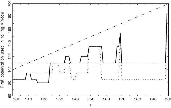
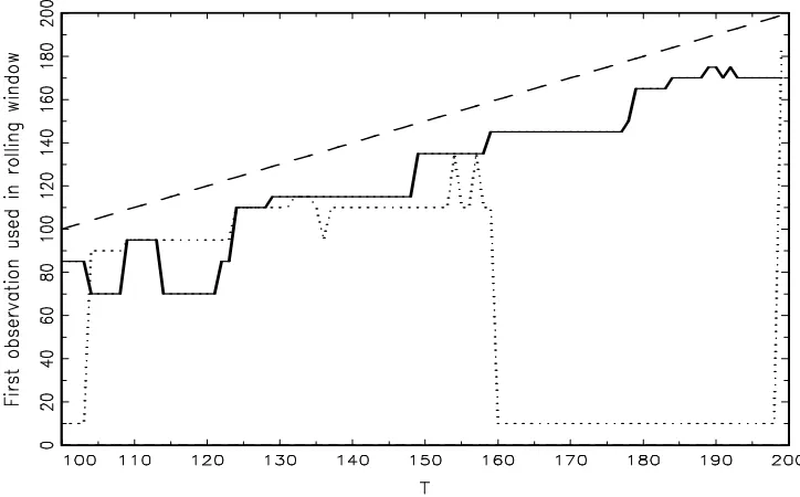
experiments used in our Monte Carlo study below. We look at rolling window forecasts. Figures 1 and 2 report the starting point (solid line) of the data selected rolling window for a structural break in the mean (Experiment 4 of our Monte Carlo study) and a unit root model (Experiment 11), respectively. The sample sizeT is 200 and the forecasting starts att0 = 100.2 For comparison,
we also report the first observation in the data-estimated rolling window when the model has no structural change (Experiment 1 in the Monte Carlo study), based on the same realisations of the noise ut, as in the previous two cases (dotted line). The vertical distance between the diagonal
(long dashes, the last observation in the window) and the starting point solid (dotted) line for a given t = 100,· · · ,200 shows the time span of observations (a graphical realisation of the tuning parameter) used for forecasting, that is t−Hˆt. It is clearly seen that, under structural change,
the estimated tuning parameter selects a much smaller sample for forecasting than in the absence of structural change. Figure 1 shows that, for the structural break (at observation 110) the data
2Details on how the parameter ˆH
Figure 1: Realisation of the data selected rolling window for a structural break. The solid line represents the starting point of the window for a structural break model with a break at observation 110 (Experiment 4 of the Monte Carlo study), and the dashed line (long dashes) shows the last observation in the window. The dashed line (short dashes) indicates the first post break observation, and the dotted line the beginning of the window when there is no structural change.
Figure 2: Realisation of the data selected rolling window for a unit root. The solid line line shows the starting point of the window for a unit root model (Experiment 11 of the Monte Carlo study), and the dashed line (long dashes) the last observation in the window. The dotted line indicates the beginning of the window when there is no structural change.
2.8
Extensions
Our proposed method extends in several practically relevant ways. In this section we briefly discuss some of these.
Nonparametric method
The above analysis presupposes a particular parametric form for the weight function. While that might be desirable from the usual motivation of parsimony, in some circumstances it will be restrictive. For example, monotonic downweighting might be counterproductive when data come from a processes that follows a finite number of regimes. Data from the same regime as that holding during the latest forecast period may be more relevant than more recent data. To account for such possibilities, we construct a nonparametric weighting scheme.
Again we focus on the simple location model (2.1) assuming that βt is some smooth
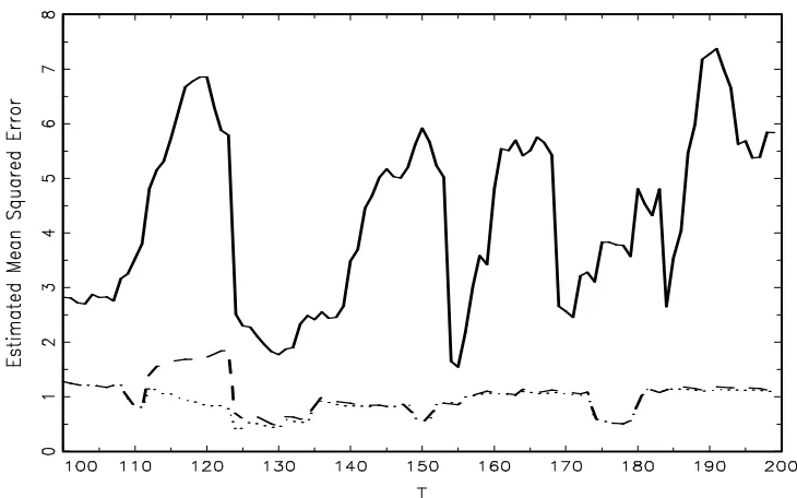
Figure 3: Realisation of the estimated MSE. The dotted line shows the MSE for the stationary case, the long-dashed line for the structural break case and the solid line for the unit root case.
form
ˆ
yt|t−1 =
Pt−1
j=1wtjyt−j. (2.30)
We wish to determine a nonparametric set of weightswT j,j = 1,· · · , T−1, such that the forecast
MSE of ˆyT|T−1 is minimised subject to PT
−1
i=1 wT j = 1. Letting ˜βt=βt−βT,
E(ˆyT|T−1−yT)2 = PT
−1
j=1 wT jβ˜T−j
2 +σ2
u
PT−1
j=1 w
2 T j.
We construct the Lagrangean
L(λ, wT1,· · · , wT ,T−1) =
PT−1
j=1 wT jβ˜T−j
2 +σ2
u
PT−1
j=1 w2T j−λ
PT−1
j=1 wT j −1
.
Taking derivatives of L w.r.t. the wT js and equating them to zero, gives equations
( ˜βT2−j+σu2)wT j + ˜βT−j
PT−1
i=1,i6=jβ˜T−iwT i =λ/2, j = 1,· · · , T −1.
We need to solve this set of equations. As a system they are written as
where ˜B = ( ˜βT−jβ˜T−k)j,k=1,...,T−1 is a (T −1)×(T −1) matrix, I is a (T −1)×(T −1) identity
matrix, wT = (wT j)j=1,···,T−1 is a (T −1)×1 vector, 1 is (T −1)×1 unit vector, B = ˜B +σuI
and Λ = (λ/2)1.
Then, wT = B−1Λ, and λ is determined such that the sum of the elements of B−1Λ is unity.
This is not an operational procedure as βT is unknown at time T−1. We suggest settingβt= ˆβt,
t= 1,· · · , T −1 and βT = ˆβT = ˆβT−1 where ˆβt denotes some estimator ofβt. This approach does
not allow for a dependent ut, but we discuss possible extensions of (2.1) below that make the
assumption of a serially uncorrelated ut more plausible.
The method can be extended to allow for time varying variancesEu2t =σu,t2 . Then, the forecast MSE takes the form
E(ˆyT|T−1−yT)2 = PT
−1
j=1 wT jβ˜T−j
2
+PT−1
j=1 w
2
T jσ2u,T−j.
Following the steps of the previous argument gives the following system of equations
( ˜B+ ˜I)wT = (λ/2)1, or BwT = Λ,
where ˜I = diagonal(σ2
u,T−1,· · · , σu,12 ) is (T −1) ×(T − 1) diagonal matrix. Once again this
procedure becomes operational by replacing σ2
u,t with an estimate. We note that estimation of βt
and σ2
u,t is discussed widely in the literature whenβt and σu,t2 are deterministic functions of time
(see, e.g., Orbe, Ferreira, and Rodriguez-Poo (2005) and Kapetanios (2007)), and is examined in Giraitis, Kapetanios, and Yates (2011) for stochastic βt.
Subsamples
Another extension allows the forecast MSE to be evaluated and minimised over different sample periods, in order to select the optimal subsample and a specific tuning parameter. This is achieved by an extended two-parameter minimisation procedure given by
QT ,kH := (T −k)−1
PT
t=k(ˆyt|t−1, H−yt)2, {H,ˆ ˆk}:= argminH∈IT,k∈{kmin,···,kmax}QT,H,k. (2.32)
The selected values of ( ˆH,kˆ) can then be used to construct forecasts based on the subsample [ˆk,· · · , T]. This value of H may be different from that obtained by the optimisation in (2.5). Such a procedure, when building forecasts, seeks for an optimal subsample yˆk,· · · , yT (‘stability
period’) and an associated optimal tuning parameter ˆH = ˆH(ˆk). Observe that for the rolling window forecast, obviously ˆH ≤ T −ˆk. However, using exponential downweighting, only data
yˆk,· · · , yT should be used.
The advantage of the two parameter procedure becomes obvious in rolling window forecasts under the break in the mean, discussed in Example 2. If the rolling window is selected using all the data in a large sample y1,· · · , yT, then it takes
√
T time lags for the forecast to switch to the postbreak data. However, the switch may be faster when less observations are used (i.e., when ˆ
Dynamic weighting
Another simple way to allow for extra flexibility in the weight function is to allow the first p
weights w1,· · · , wp (p≥0) to vary freely by specifying
˜
wtj,H =
wj, j = 1,· · · , p,
K(j/H), j =p+ 1,· · · , t−1, H ∈IT,
(2.33)
and standardising the weights: wtj,H = ˜wtj,H/
Pt−1
j=1w˜tj,H
. This allows the first few lags ofyt to
enter freely into the forecast rather than through a given parametric function, akin to an estimated AR process. Then, QT can be minimised jointly over H,w˜1,· · · ,w˜p, and, potentially, evenp.
Conditional mean modelling
The location set-up in (2.1) does not allow for explicit conditional mean modelling. In this subsection we address this issue. It would be good if our analysis allows both the use of a generic model of the conditional mean of the process and robust forecasting around that model. Specifically, we would like to assume that the forecaster has a preferred model of the conditional mean which is known (at least up to a finite vector of unknown parameters), and then discuss how our robust adaptive forecasting methods can be applied to the residual from such a model. This allows considerable generality, and in practice allows application to realistic conditional mean models such as the widely used AR model.
In the conditional mean framework, one has a generic forecasting model of the form
xt=g(zt) +yt (2.34)
of the variable of interestxtthat produces forecastsg(zt+1) based on a vector of predictor variables
that may contain lags of xt, or other generated variables such as, e.g., dummies to account for
structural change. The process yt in (2.34) is the part of xt unexplained by g(zt). Assuming
that the conditional mean function g has a known parametric structure up to an unknown finite dimensional parameter, fitting it to xt gives rise to a parametric forecasting model. Clearly, such
a model can be misspecified and may suffer problems associated with the presence of structural change in xt, as discussed in the introduction. We will abstract from specification and estimation
issues associated withg. This is because we wish to keep our discussion as general as possible and not related to the exact structure of g. Additionally, the presence of structural change in xt is
likely to complicate considerably any rigorous analysis of estimators of the unknown parameters. Moreover, our analysis of forecasting yt will efficiently exploit any persistence remaining in yt.
Hence, it is sufficient to assume that fitting the modelg(zt) to xt producesyt with an unspecified
persistent structure that may combine dependence, trends and breaks. Once (2.34) is posited and the possibility allowed of suboptimal forecasts byg(zt+1) due to structural change, it is important
to consider ways in which additional forecasting of yt may produce a superior forecast of xt. In
known or estimated by any of the currently available methods in the literature. However, under ongoing structural change, the properties of such an estimator may be difficult to determine.
In summary, for any given forecast ˆxt of xt, based on information available up to time t−1,
we shall write xt = ˆxt +yt, t = 1,· · · , T. Then we can use our robust methods to produce
a forecast ˆyT+1 of yT+1, based on yt = xt−xˆt, t ≤ T and define the final forecast of xT+1 as
x(f orecast)T+1 = ˆxT+1+ ˆyT+1. For example, we may set ˆxt≡0, and thenyt=xt, t≤T. Alternatively,
we can fit to the data,xt, some model of the formg(xt−1, xt−2· · ·) and after obtaining its estimate,
ˆ
g, we arrive at ˆxt = ˆg(xt−1, xt−2· · ·). It may be the case, as it sometimes is in policy institutions
such as central banks, that g or ˆxt is obtained using informal judgements by policymakers. Note
that any neglected dynamics or errors produced by such a fitting process will be accumulated in
yt and used subsequently to forecastyT+1.
2.9
Theoretical conclusions
We conclude this section by noting some important implications of our analysis.
First, the dominant tendency in the forecasting literature of using models developed for non-forecast purposes, such as to generate impulse responses or policy analysis, may be counterproduc-tive. Our arguments suggest that if good forecasting is the aim, then forecasting by averaging or appropriately downweighting past data, without engaging in further modelling, is a viable strategy. Second, appropriately downweighting past can provide a general approach for handling trends of any nature. Our theoretical results show that this method applies for stochastic, linear or nonlinear deterministic trends and structural breaks without knowledge of the nature of the trend. It is therefore a tractable method for forecasting the levels of apparently nonstationary processes. As a result it bypasses difficult problems of combining appropriate detrending of level series with the subsequent forecasting of stationary processes. Importantly, the proposed forecasting approach continues to be valid if a series is actually stationary.
Finally, while theoretical results, such as, e.g., Remark 1, and small sample evidence indi-cate that an exponential kernel has theoretical advantages over a rolling window and is a very good choice in general, in a particular empirical application another kernel function may still be preferable. It is then worth noting that the MSE minimisation procedure determining the rate of downweighing past data can be used to select the kernel function, K, that produces the lowest MSE, among a set of admissible kernel functions.
3
Monte Carlo study
In this section we explore the finite sample performance of the forecasting strategies discussed in the previous section. We consider Monte Carlo experiments for the forecast of yT+1 based on
the sample y1,· · · , yT for a number of specific designs for the simple location model (2.1) with
models with short memory dynamics. We analyse one-step ahead forecasts where the benchmark is the sample mean forecast ˆybenchmark,T+1 =T−1
PT
t=1ytor an autoregressiveAR(1) forecast. The
benchmarks disregard the possibility of structural change. We also consider a benchmark of the last available observation forecast, optimal when the process is a random walk. We compare the performance of the various forecasts in terms of relative MSE.
Design: data generating processes. We consider the following location shift model (2.1) for generating the data:
yt=βt+ut, t= 1,· · ·, T,
whereutis either a standard normal IID(0,1) noise, or anAR(1) process with parameterρ= 0.7 or
-0.7 and standard normal i.i.d. innovations. The process βt is either a deterministic or stochastic
trend, or a process with a break in the mean. We consider the following data generating processes, denoted in tables as Ex1–Ex12:
1. yt =ut. 7. yt= 2T−1/2
Pt
i=1vi+ 3ut.
2. yt = 0.05t+ 5ut. 8. yt= 2T−1/2Pti=1vi+ut.
3. yt = 0.05t+ 3ut. 9. yt= 0.5
Pt
i=1vi+ 3ut.
4. yt =
ut, t≤t0 =T /2,
1 +ut, t > t0.
10. yt= 0.5
Pt
i=1vi+ut.
5. yt = 2 sin (2πt/T) + 3ut. 11. yt=
Pt
i=1vi.
6. yt = 2 sin (2πt/T) +ut. 12. yt=Pti=1ui,
where vt is a standard normal IID(0,1) sequence. This selection of deterministic trends provides
a variety of shaped functions driving the structural change in the unconditional mean of yt.
Ex1 is the case of no structural change. Here, as long as the noiseutis an i.i.d. or very weakly
dependent process, the benchmark sample mean forecast should do best, and the robust methods at most should not lag far behind the benchmark. If ut is a dependent process with persistent
autoregressive dynamics then theARbenchmark should do best. Further, in this case, the robust forecast with EWMA weights should outperform the sample mean benchmark and rolling window (see Remark 1). Theory indicates that the exponential weights should outperform the rolling window, but it leaves open the possibility that the rolling window can outperform the benchmark when a stationary process yt becomes persistent.
The functional form in Ex2 and Ex3 is a linear monotonic trend. While such trends may be unrealistic, at least for processes which have been detrended by applying filters or differencing, they provide a useful benchmark. Further, these trends are sufficiently subtle and minor to be swamped visually by the noise process. We consider different values for the variance of the noise process to explore such effects. The purpose of Ex4 is to introduce a break in the mean, to see if our robust methods can help under traditional structural change specifications. The break occurs at timet0 =T /2, and the post-break time is greater than
√
Functions in Ex5 and Ex6 represent smooth cyclical bounded trends. These are more likely to remain after standard detrending and provide a realistic scenario. Moreover, wider oscillation of the trend in Ex6 relative to the variance of the noise process seems to lead to a stronger deterioration of the performance of the benchmark.
Next, Ex7 and Ex8 deal with a bounded stochastic trend βt which is relevant for popular
time-varying coefficient specifications in the macroeconometric and forecasting literature, while
Ex9 andEx10 deal with a random walk (unit root) process, observed under noise. Finally, Ex11 andEx12 consider two versions of a standard random walk model, differing only in the persistence of the noise processes.
3.1
Forecast methods
We examine the robust forecasting methods using three classes of parametric weight functions.
Rolling window. This uses flat weights,
wtj,H =H−1I(1≤j ≤H), j = 1,· · · , t−1, for H < t, and
wtj,H = (t−1)−1I(1≤j ≤t−1)), for H ≥t,
giving equal weight to recent data and zero weight to older data. We denote it in the tables below byRolling H where H is the window size.
Exponential (EWMA). This uses weights
wtj,ρ=ρt−j/
Pt−1
k=1ρk
, 1≤j ≤t−1, with 0< ρ < 1.
Here the main weight is placed on the last few data points, downweighting others to zero ex-ponentially fast when ρ is small, and more equally when ρ is close to 1. We refer to this as
Exponential ρ.
Polynomial method. This uses weights
wtj,α = (t−j)−α/
Pt−1
k=1k
−α, 1≤j ≤t−1 with α >0.
The past is downweighted at a slower slower rate than with exponential weights. We refer to it as
P olynomial α.
Methods with fixed tuning parameters. We consider forecasts with both fixed values of
H and ρ, and data selected values ˆH, ˆρ and ˆα for the tuning parameters. With polynomial weights we do not examine the fixed value cases. We set H = 20,30 for rolling window and for exponential weights ρ = 0.99,0.95,0.9,0.8,0.7 and 0.5. Using fixed values allows us to compare the performance of the forecast with a data-tuned parameter with the best (smallest Monte Carlo forecast MSE) among the fixed cases. Our objective is to verify in simulations that these two MSEs,ωT ,Hˆ and ωT ,Hopt, are comparable, as indicated by Corollaries 1 to 3.
Rolling (ˆk,Hˆ) method. This is the rolling window forecast where ˆk and ˆH are selected min-imising QT ,kH in H and k as in (2.32), referred to as Rolling (ˆk,Hˆ).
Averaging method. The final robust method we examine is the averaging method of rolling window forecasts over different periods advocated by Pesaran and Timmermann (2007):
¯
yT+1|T =
1
T
T
X
H=1
ˆ
yT+1|T , H, yˆT+1|T , H =
1
H
T
X
t=T−H+1
yt. (3.1)
It combines rolling window forecasts of yT+1 using all possible windows that include the last
available observation. A characteristic of this method is that it does not require selection of any tuning parameters apart from the mimimum sample size used for forecasting, which is usually of minor significance. We refer to this as Averaging.
Dynamic weighting method. This uses the weights defined in (2.33) withp= 1 and exponential
K. We refer to it as Dynamic weighting.
Residual methods. We apply three methods to forecast xt = g(zt) +yt, t = 1,· · · , of (2.34).
They fit to xt the AR(1) dynamicsg(zt) =φxt−1 and forecast residualsyt by either a parametric
or nonparametric method. The forecast of xt+1 based on x1,· · · , xt is ˆxt+1 = ˆφxt+ ˆyt+1|t,Hˆ.
Exponential AR method. It estimates the autoregressive parameterφand the tuning parameter
H jointly by minimising the forecast error QT ,H = QT ,Hφ computed using yt = xt−φxt−1 with
exponential weights. We refer to it as Exponential AR.
The other two methods are two-stage methods, where the autoregressive parameter φ at xt−1
is estimated by OLS separately from the parameters associated with forecastingyt.
Exponential residual method. It forecasts residuals ˆyt =xt−φxˆ t−1 using exponential weights
producing ˆH and the forecast ˆyt+1|t,Hˆ. We refer to it as Exponential Residual.
Nonparametric residual method. It forecasts residuals ˆyt =xt−φxˆ t−1 using the nonparametric
forecast method. We refer to it as Nonparametric Residual.
3.2
Monte Carlo results
We choose a particular forecast starting point at time t0 by any given method. Then one-step
ahead forecasts yt0|t0−1, H,· · · , yt|t−1, H,t=t0, ..., T, are computed. The forecast evaluation period
ends at T. Note that all forecasts for t are produced using only information up to t−1. To compare different forecast methods, as the performance criterion we use the forecast MSE relative to the benchmark of the sample mean of all data (M SERR). For method i, we computeM SEi =
(T−t0)−1
PT t=t0(ˆy
(i)
t|t−1−yt)
2 and define the relative M SE
RR = M SEM SE0i whereM SE0 corresponds to
the benchmark forecast by the sample mean. For all experiments, forecasting starts at t0 = 100,
and the sample size isT = 200. M SERR below unity shows that the forecast method outperforms
the sample mean. We carry out 200 replications and report the average M SERR over these.
Table 1: Monte Carlo Results. T = 200. One-Step Ahead Forecasts. ut ∼ IID(0,1). Table
reports relative mean squared error using a full sample mean benchmark
Experiments
Method Ex1 Ex2 Ex3 Ex4 Ex5 Ex6 Ex7 Ex8 Ex9 Ex10 Ex11
Exponential ρ= ˆρ 1.085 0.699 0.436 0.791 0.802 0.253 1.029 0.691 0.622 0.212 0.042
Rolling H= ˆH 1.066 0.694 0.448 0.807 0.804 0.276 1.005 0.696 0.627 0.272 0.153
Rolling H= 20 1.039 0.658 0.413 0.762 0.759 0.264 0.977 0.668 0.618 0.323 0.268
H= 30 1.027 0.654 0.420 0.768 0.764 0.312 0.965 0.685 0.659 0.403 0.373
Exponential ρ= 0.99 1.003 0.736 0.570 0.833 0.836 0.556 0.964 0.766 0.750 0.592 0.562
ρ= 0.95 1.040 0.656 0.412 0.751 0.759 0.258 0.972 0.652 0.595 0.271 0.192
ρ= 0.90 1.102 0.690 0.426 0.778 0.795 0.242 1.023 0.667 0.592 0.211 0.104
ρ= 0.80 1.234 0.772 0.472 0.861 0.892 0.263 1.142 0.733 0.645 0.196 0.062
ρ= 0.70 1.414 0.888 0.538 0.983 1.028 0.299 1.304 0.833 0.731 0.208 0.048
ρ= 0.50 1.947 1.231 0.737 1.352 1.431 0.411 1.783 1.137 0.998 0.268 0.041
Averaging 1.003 0.747 0.589 0.848 0.844 0.583 0.967 0.781 0.774 0.636 0.619
N onparametric 1.102 0.671 0.415 0.770 0.778 0.239 1.015 0.667 0.595 0.242 0.155
P olynomial α= ˆα 1.025 0.726 0.488 0.807 0.817 0.310 0.987 0.695 0.640 0.322 0.149
Rolling H= ˆH,k= ˆk 1.061 0.720 0.473 0.812 0.825 0.283 1.011 0.699 0.636 0.243 0.106
Dynamic W eighting 1.162 0.719 0.452 0.807 0.822 0.260 1.082 0.711 0.630 0.214 0.045
Exponential AR 1.107 0.729 0.456 0.830 0.832 0.265 1.074 0.720 0.642 0.219 0.044
Exponential Residual 1.093 0.707 0.474 0.815 0.815 0.316 1.026 0.720 0.660 0.245 0.044
N onparametric Residual 1.109 0.697 0.470 0.795 0.802 0.312 1.025 0.708 0.650 0.240 0.044
Last Observation 1.951 1.234 0.738 1.355 1.435 0.412 1.787 1.140 1.001 0.269 0.041
AR 1.000 0.805 0.599 0.826 0.870 0.381 0.978 0.844 0.790 0.310 0.052
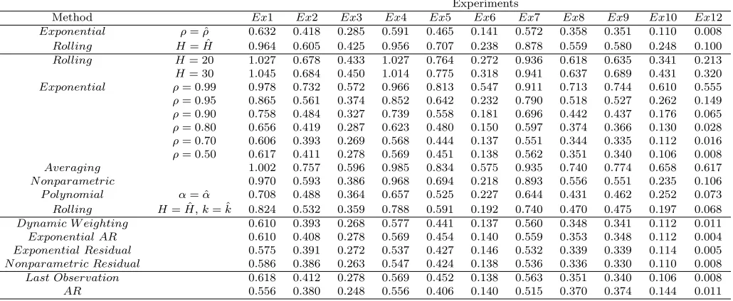
Table 2: Monte Carlo Results. T = 200. One-Step Ahead Forecasts. ut ∼ AR(0.7). Table
reports relative mean squared error using a full sample mean benchmark
Experiments
Method Ex1 Ex2 Ex3 Ex4 Ex5 Ex6 Ex7 Ex8 Ex9 Ex10 Ex12
Exponential ρ= ˆρ 0.632 0.418 0.285 0.591 0.465 0.141 0.572 0.358 0.351 0.110 0.008
Rolling H= ˆH 0.964 0.605 0.425 0.956 0.707 0.238 0.878 0.559 0.580 0.248 0.100
Rolling H= 20 1.027 0.678 0.433 1.027 0.764 0.272 0.936 0.618 0.635 0.341 0.213
H= 30 1.045 0.684 0.450 1.014 0.775 0.318 0.941 0.637 0.689 0.431 0.320
Exponential ρ= 0.99 0.978 0.732 0.572 0.966 0.813 0.547 0.911 0.713 0.744 0.610 0.555
ρ= 0.95 0.865 0.561 0.374 0.852 0.642 0.232 0.790 0.518 0.527 0.262 0.149
ρ= 0.90 0.758 0.484 0.327 0.739 0.558 0.181 0.696 0.442 0.437 0.176 0.065
ρ= 0.80 0.656 0.419 0.287 0.623 0.480 0.150 0.597 0.374 0.366 0.130 0.028
ρ= 0.70 0.606 0.393 0.269 0.568 0.444 0.137 0.551 0.344 0.335 0.112 0.016
ρ= 0.50 0.617 0.411 0.278 0.569 0.451 0.138 0.562 0.351 0.340 0.106 0.008
Averaging 1.002 0.757 0.596 0.985 0.834 0.575 0.935 0.740 0.774 0.658 0.617
N onparametric 0.970 0.593 0.386 0.968 0.694 0.218 0.893 0.556 0.551 0.235 0.106
P olynomial α= ˆα 0.708 0.488 0.364 0.657 0.525 0.227 0.644 0.431 0.462 0.252 0.073
Rolling H= ˆH,k= ˆk 0.824 0.532 0.359 0.788 0.591 0.192 0.740 0.470 0.475 0.197 0.068
Dynamic W eighting 0.610 0.393 0.268 0.577 0.441 0.137 0.560 0.348 0.341 0.112 0.011
Exponential AR 0.610 0.408 0.278 0.569 0.454 0.140 0.559 0.353 0.348 0.112 0.004
Exponential Residual 0.575 0.391 0.272 0.537 0.427 0.146 0.532 0.339 0.339 0.114 0.005
N onparametric Residual 0.586 0.386 0.263 0.547 0.424 0.138 0.536 0.336 0.330 0.110 0.008
Last Observation 0.618 0.412 0.278 0.569 0.452 0.138 0.563 0.351 0.340 0.106 0.008
AR 0.556 0.380 0.248 0.556 0.406 0.140 0.515 0.370 0.374 0.144 0.011
standard normal process, whereas in Tables 2 and 3, the ut are dependent variables, generated
by stationary AR(1) processes with parameters ρ= 0.7 and ρ=−0.7 and i.i.d. standard normal innovations respectively.
The first column, labelled Ex1, corresponds to the stationary case yt = ut. In the i.i.d.
case, as expected, the sample mean outperforms the forecasts for each method, especially those penalised by the loss of information from strong discounting. However, for sufficiently dependent
ut, discounting improves the forecast as indicated by Remark 1.
[image:22.612.75.590.382.594.2]sense that theM SERR is considerably below unity. Further, the full sample autoregressive model
although better than the sample mean forecast in the majority of cases is also beaten by down-weighting methods in several cases, particularly where there is a location shift or autoregressive dynamics. Generally, all these methods are useful, including the rolling window and averaging method. In the case of a fixed tuning parameter, for the model with a strong trend, the largest reduction of M SERR comes from the exponential weights with the highest discount rates.
Al-though the tuned exponential weights are not the best, they are where they should be according to theory: comparable to the best fixed value methods and never among the poor performers. Note, e.g., that the exponential weights with a ρ= 0.9 fixed discount can perform both very well and considerably worse than the tuned exponential weights in a number of cases, illustrating the importance of data-dependent tuning.
Given that optimal fixed ρfor exponential weights cannot be observed in practice, our simula-tion study suggests the efficiency and usefulness of data based downweighting. The nonparametric method similarly offers a powerful alternative, for i.i.d. noise ut slightly beating the tuned
pa-rameter methods in many cases. However, being designed for an i.i.d. noise ut, in case of a
dependent AR(1) noise this method is outperformed by the parametric tuning methods, unless coupled with an initial AR correction. It is also worth mentioning that while the benchmark full sample AR forecast is a good competitor in many cases, there are circumstances such as, for example, i.i.d. noise or autoregressive noise with negative autoregressive coefficients where it can perform considerably worse than robust downweighting methods.
Comparing exponential, rolling window and polynomial methods, the exponential method outperforms rolling windows while the latter beats polynomial windows when the noise ut is
dependent and is outperformed by it when the noise is i.i.d. The averaging method outperforms the benchmark but is beaten by the rolling windows with data selected ˆH. The rolling window forecast using a data dependent window, ˆH, and an evaluation period [ˆk, T], is equivalent to a rolling window with ˆH and k= 1 under the i.i.d. noise, but outperforms it when the noise, ut, is
dependent.
It is worth noting that, in applications, one could select from a set of available forecasts with data dependent and fixed discounting rates, the one minimising the criterion function QT ,H of
(2.5), and respectively, the forecast MSE, ωT ,Hˆ ∼ QT,Hˆ. This possibility illustrates the wide
relevance of our cross-validation approach.
Table 3: Monte Carlo Results. T = 200. One-Step Ahead Forecasts. ut ∼ AR(−0.7). Table
reports relative mean squared error using a full sample mean benchmark
Experiments
Method Ex1 Ex2 Ex3 Ex4 Ex5 Ex6 Ex7 Ex8 Ex9 Ex10 Ex12
Exponential ρ= ˆρ 1.007 0.691 0.435 1.005 0.784 0.263 0.965 0.668 0.651 0.202 0.141
Rolling H= ˆH 1.055 0.698 0.444 1.059 0.791 0.271 0.976 0.670 0.658 0.241 0.213
Rolling H= 20 1.040 0.664 0.412 1.045 0.759 0.269 0.959 0.658 0.644 0.307 0.289
H= 30 1.026 0.662 0.419 1.028 0.764 0.317 0.948 0.681 0.673 0.385 0.372
Exponential ρ= 0.99 1.012 0.747 0.571 1.013 0.846 0.563 0.960 0.768 0.779 0.594 0.566
ρ= 0.95 1.088 0.691 0.428 1.088 0.787 0.272 0.995 0.662 0.642 0.258 0.227
ρ= 0.90 1.212 0.765 0.468 1.212 0.864 0.269 1.102 0.705 0.675 0.203 0.158
ρ= 0.80 1.490 0.940 0.573 1.493 1.059 0.321 1.353 0.849 0.809 0.203 0.136
ρ= 0.70 1.903 1.201 0.732 1.911 1.354 0.409 1.728 1.077 1.024 0.238 0.146
ρ= 0.50 3.326 2.102 1.284 3.358 2.373 0.713 3.021 1.873 1.776 0.387 0.217
Averaging 1.007 0.756 0.587 1.008 0.852 0.589 0.961 0.783 0.807 0.645 0.615
N onparametric 1.074 0.694 0.426 1.078 0.787 0.249 1.000 0.658 0.635 0.222 0.193
P olynomial α= ˆα 1.001 0.801 0.547 1.001 0.873 0.353 0.980 0.730 0.718 0.293 0.251
Rolling H= ˆH,k= ˆk 1.052 0.739 0.464 1.055 0.832 0.277 1.004 0.686 0.663 0.217 0.173
Dynamic W eighting 0.826 0.399 0.251 0.787 0.448 0.158 0.615 0.430 0.424 0.162 0.131
Exponential AR 0.581 0.399 0.252 0.563 0.449 0.161 0.575 0.438 0.433 0.162 0.122
Exponential Residual 0.573 0.434 0.393 0.557 0.482 0.368 0.559 0.541 0.559 0.298 0.194
N onparametric Residual 0.585 0.419 0.381 0.565 0.465 0.360 0.543 0.534 0.549 0.292 0.192
Last Observation 3.340 2.111 1.289 3.372 2.383 0.716 3.033 1.881 1.784 0.389 0.218
AR 0.527 0.790 0.737 0.506 0.745 0.522 0.634 0.786 0.797 0.336 0.200
4
Empirical illustration
In this section we examine how our methods would have fared when applied to a wide range of US quarterly data series.3 We are not trying to establish the best methods for particular data series,
but instead to get an impression of whether the issues identified above are important in practice. Although not required with our methodology, so as not to disadvantage the simple location and an AR(1) benchmarks in all cases we transform series to stationarity. We use data on 97 US series for the US, taken from Eklund, Kapetanios, and Price (2010). The dataset includes real activity, prices and financial variables among others. Appendix C of Eklund, Kapetanios, and Price (2010) lists the series. The data span 1960Q1 to 2008Q3. We evaluate one step ahead forecasts over a long period starting in 1992Q2 and ending in 2008Q3. For each series, we compare MSEs to those from the full sample benchmark simple location and AR(1) models.4
The robust methods we report are those in the Monte Carlo study, and include rolling win-dow forecasts, averaging across estimation periods, exponentially weighted moving average fore-casts, polynomially weighted moving average forecasts and forecasts produced using nonparametric weights and residuals.
Table 4 contains the results. We report the median and mean M SERR relative to the full 3We take no account of real-time data revisions.
4The simple location model benchmark is the baseline model in our exposition and can perform well as a
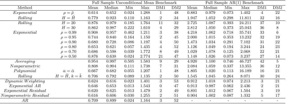
Table 4: Empirical relative mean squared error results for the US data with a full sample uncon-ditional mean and AR(1) forecast as benchmarks.
Full Sample Unconditional Mean Benchmark Full Sample AR(1) Benchmark
Method Mean Median Min Max DM1 DM2 Mean Median Min Max DM1 DM2
Exponential ρ= ˆρ 0.614 0.652 0.024 1.288 1 48 0.883 0.979 0.073 1.402 4 22
Rolling H= ˆH 0.779 0.923 0.110 1.163 2 34 1.947 1.052 0.298 11.811 32 16
Rolling H= 20 0.876 0.979 0.185 1.764 11 32 2.725 1.087 0.393 24.211 37 10
H= 30 0.862 0.987 0.222 1.610 4 29 2.812 1.050 0.373 25.043 36 8
Exponential ρ= 0.99 0.908 0.957 0.462 1.211 3 38 4.218 1.062 0.718 35.741 33 6
ρ= 0.95 0.744 0.840 0.164 1.150 2 45 2.000 1.015 0.353 13.232 32 19
ρ= 0.90 0.680 0.728 0.086 1.197 4 50 1.473 1.034 0.291 7.102 31 22
ρ= 0.80 0.653 0.621 0.057 1.435 4 52 1.126 1.049 0.194 3.244 24 23
ρ= 0.70 0.686 0.598 0.039 1.772 8 49 1.029 1.078 0.125 2.068 22 21
ρ= 0.50 0.876 0.638 0.024 2.774 21 47 1.148 1.026 0.073 3.237 27 14
Averaging 0.954 0.997 0.505 1.583 9 29 4.920 1.100 0.746 46.727 42 5
N onparametric 0.808 0.904 0.111 1.738 7 31 2.084 1.059 0.337 13.355 36 12
P olynomial α= ˆα 0.667 0.682 0.055 1.207 1 48 1.805 1.020 0.113 16.189 16 21
Rolling H= ˆH,k= ˆk 0.706 0.792 0.089 1.135 2 50 1.545 1.045 0.264 8.071 30 24
Dynamic W eighting 0.624 0.616 0.023 1.401 3 53 0.912 1.018 0.074 2.213 3 21
Exponential AR 0.646 0.653 0.013 1.543 0 47 0.913 0.987 0.062 2.436 2 21
Exponential Residual 0.620 0.625 0.013 1.479 2 49 0.891 1.012 0.067 1.504 3 19
N onparametric Residual 0.616 0.606 0.030 1.255 2 51 0.904 1.002 0.087 1.332 5 17
AR 0.709 0.899 0.024 1.164 3 52 - - -
-sample mean (equal weight) benchmarks. We also include the minimum and maximum M SERR.
DM1 and DM2 report the number of significant Diebold-Mariano tests where the null is equality of the downweighting method and the benchmark. The alternative for DM1 is that the benchmark is the better forecast, and for DM2 that the downweighting method is superior. As in most cases for one of the two comparator models a form of rolling estimation is involved, the use of this test is valid (Giacomini and White (2005)).
In almost all cases, the data-dependent downweighting methods beat the sample mean bench-mark. The median reduction in the optimised EWMA downweighting forecast is large, reaching over 30%. But this simple benchmark will not usually be applied in practice, as typically forecasts accounting for some dynamics are employed. Thus of much more interest is the more challenging AR benchmark.
The median statistics with respect to the AR model are typically greater than one, showing that the proposed methods fail to outperform a full sample AR. The natural interpretation of this is that only a minority of series suffer from structural change. Notwithstanding this, we note that the optimised exponential and the exponential AR beat the benchmark at the median, and elsewhere the forecast performance penalty at the median is small. This is particularly true for the dynamic methods (dynamic weighting and residual methods). The implication is that in this sample our methods are safe to use, in the sense that typically they will be, at worst, only slightly inferior to a full sample AR benchmark.
of course, is that one fixed weight is unlikely to be right for all series. The data-dependent and fixed window rolling method also does poorly, as does the averaging method. Neither are the nonparametric and optimised polynomial methods particularly successful. But by contrast, in general the optimised EWMA downweighting and dynamic models (the dynamically weighted and residual based methods) do well, and we concentrate our discussion on these.
The mean M SERR of the optimised EWMA and dynamic methods is uniformly below the
median, indicating that there is a predominance of well performing models and that sometimes, when structural change occurs, there are very large benefits to be had from the use of our proposed methods relative to an AR benchmark. The mean reduction in MSE is large enough to be practi-cally important. In the best cases, for the dynamic models the improvement is sensational, with MSEs of less that 0.07. The exponential method is also an outstanding performer. In the worst cases, the optimised EWMA and the dynamic methods have MSEs between 1 and 1.5. While large, these are generally much lower than for the non-optimised (fixed tuning parameter) meth-ods. These impressions are confirmed by formal tests. For the data-dependent exponential and the dynamic models in between 18 and 23% of cases the proposed method is significantly better than the AR benchmark, with less than 5% of cases where the benchmark is significantly better than the proposed robust method. This is strong evidence in support of the practical utility of data-dependent downweighting dynamic models.
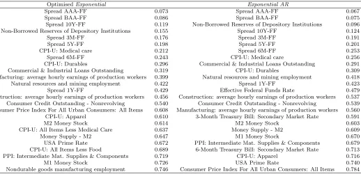
Table 5 reports the series where the outperformance is most pronounced. It includes the 20 series with the smallest MSEs compared to the AR(1) for optimised Exponential and Exponential AR methods. There are very large improvements relative to the benchmark for all of these series, which are never unimportant practically and in some cases dramatic. The methods are particularly useful for forecasting spreads and inflation series. This is further strong evidence supporting the use of the optimised EWMA and dynamic methods.
5
Conclusions
Table 5: 20 series with the smallest relative M SERR for optimised Exponential and Exponential
AR forecast and AR(1) forecast benchmark
OptimisedExponential Exponential AR
Spread AAA-FF 0.073 Spread AAA-FF 0.067
Spread BAA-FF 0.086 Spread BAA-FF 0.075
Spread 10Y-FF 0.119 Non-Borrowed Reserves of Depository Institutions 0.096
Non-Borrowed Reserves of Depository Institutions 0.155 Spread 10Y-FF 0.124
Spread 3M-FF 0.176 Spread 3M-FF 0.191
Spread 5Y-FF 0.198 Spread 5Y-FF 0.201
CPI-U: Medical care 0.212 Spread 6M-FF 0.253
Spread 6M-FF 0.243 CPI-U: Medical care 0.256
CPI-U: Durables 0.296 Commercial & Industrial Loans Outstanding 0.291
Commercial & Industrial Loans Outstanding 0.319 CPI-U: Durables 0.309
Manufacturing: average hourly earnings of production workers 0.399 Natural resources and mining employment 0.418
Natural resources and mining employment 0.422 Spread 1Y-FF 0.423
Spread 1Y-FF 0.429 Effective Federal Funds Rate 0.479
Construction: average hourly earnings of production workers 0.456 Construction: average hourly earnings of production workers 0.537 Consumer Credit Outstanding - Nonrevolving 0.540 Consumer Credit Outstanding - Nonrevolving 0.539 Consumer Price Index For All Urban Consumers: All Items 0.608 Manufacturing: average hourly earnings of production workers 0.560
CPI-U: Apparel 0.610 3-Month Treasury Bill: Secondary Market Rate 0.591
M2 Money Stock 0.614 M2 Money Stock 0.603
CPI-U: All Items Less Medical Care 0.637 Money Supply - M2 0.609
Money Supply - M2 0.647 M1 Money Stock 0.670
USA Prime Rate 0.672 PPI: Intermediate Mat. Supplies & Components 0.679
CPI-U: All Items Less Food 0.689 6-Month Treasury Bill: Secondary Market Rate 0.713
PPI: Intermediate Mat. Supplies & Components 0.719 CPI-U: Apparel 0.716
M1 Money Stock 0.726 USA Prime Rate 0.740
Nondurable goods manufacturing employment 0.746 Consumer Price Index For All Urban Consumers: All Items 0.784
evidence suggest that exponential weighting may be most helpful and efficient, and that data selected tuning can provide a useful framework for avoiding large forecast errors. An especially useful finding is that our methods coupled with simple dynamic modelling, such as a low-order autoregressive structure, can provide great improvements over standard forecasting methods in the presence of structural change, while having small costs in its absence.
The simulation study and the empirical exercise using a large number of US macroeconomic series show that fixed discount EWMA weighting, with a low discount rate, is often good, but is outperformed consistently by the data selected downweighting. Not all series exhibit breaks, but in many cases forecast performance is enhanced substantially and significantly relative to a full sample AR forecast, without a large penalty in other cases. Overall, we find strong support for our approach, motivated by the impossibility of knowing the optimal degree of discounting ex ante.
A
Appendix: Proofs
A.1
Proof of Theorems 1-3 and Corollaries 1-4
In this section we establish the claims of Theorems 1-3 about QT ,H and ωT ,H for yt = βt+ut,