Ernesto Estrada1, Sandro Meloni2,3, Matthew Sheerin1, Yamir Moreno2,3,4
1Department of Mathematics & Statistics, University of Strathclyde, 26 Richmond Street, Glasgow G1 1XH, UK, 2Department of Theoretical Physics, University of Zaragoza, 50018 Zaragoza, Spain,
3Institute for Biocomputation & Physics of Complex Systems (BIFI),
University of Zaragoza, 50018 Zaragoza, Spain, and
4Complex Networks and Systems Lagrange Lab, Institute for Scientic Interchange, Turin, Italy.
The use of network theory to model disease propagation on populations introduces important elements of reality to the classical epidemiological models. The use of random geometric graphs (RGG) is one of such network models that allows for the consideration of spatial properties on disease propagation. In certain real-world scenarioslike in the analysis of a disease propagating through plantsthe shape of the plots and elds where the host of the disease is located may play a fundamental role on the propagation dynamics. Here we consider a generalization of the RGG to account for the variation of the shape of the plots/elds where the hosts of a disease are allocated. We consider a disease propagation taking place on the nodes of a random rectangular graph (RRG) and we consider a lower bound for the epidemic threshold of a Susceptible-Infected-Susceptible (SIS) or Susceptible-Infected-Susceptible-Infected-Recovered (SIR) model on these networks. Using extensive numerical simulations and based on our analytical results we conclude that (ceteris paribus) the elongation of the plot/eld in which the nodes are distributed makes the network more resilient to the propagation of a disease due to the fact that the epidemic threshold increases with the elongation of the rectangle. These results agree with accumulated empirical evidence and simulation results about the propagation of diseases on plants in plots/elds of the same area and dierent shapes.
I. INTRODUCTION
The study of epidemiological models on networks is one of the areas that has observed a major development in the application of network theory to real-world problems [1]. The discovery of the fact that networks with fat-tailed degree distributions do not display an epidemic threshold in the asymptotic limit is a relevant example of how the connectivity pattern of interacting agents can dramatically change the course of an epidemic [2, 3]. The use of network theory in epidemiological models provides a way to incorporate the individual-level heterogeneity necessary for the mechanistic understanding of the spread of infectious disease. These characteristics are very attractive for the application of network epidemiological models in ecology on the dierent spatial and temporal scales.
Although there has been many succesful applications of network theory to human and animal epidemiology, the situation is a little less developed for epidemic on plants. Ten years ago Jeger et al. [4] recognized the relatively low use of network theory for studying plant diseases. Since then, more theoretical developments have been presented in the literature. These models include the important description of the geometric constraints in which the pathogen is spreading as well as stochasticity and several sources of heterogeneity in the transmission of infection [58].
In order to consider spatial eects in the transmission of diseases it is possible to consider spatial networks that treat interactions as a continuous variable that decays with increasing distance or by distributing randomly and independently a set of vertices on the Euclidean plane to represent the relative spatial location of individual hosts or habitat patches. The second kind of model is based on random geometric graphs (RGGs) [912], in which each node is randomly assigned geometric coordinates and then two nodes are connected if the (Euclidean) distance between them is smaller than or equal to a certain thresholdr. Random geometric graphs have found applications to model populations which are geographically constrained in a certain region [1318], which oer many valuable features over other types of random graphs [19, 20]. Brooks et al. [21] have used RGGs to model the interactions between the anther smut fungus and re pink using temporal data that spans 7 years of eld studies. They have concluded that the use of spatially explicit network models can yield important insights into how heterogeneous structure promotes the persistence of species in natural landscapes.
When studying the propagation of diseases in plants there is an important factor that needs to be taken into account. It is obvious that plants are not as mobile as humans and animals, thus they reach lower levels of mixing in a given population due to mobility. The immediate consequence of this lack of mobility is the fact that the shape of the plot or eld in which the plants are distributed may signicantly aect disease dynamics. In fact, there is both empirical and theoretical evidence that supports this hypothesis [2230]. In general, it has been suggested that square plots and elds favored higher spreading of plant diseases than elongated ones of the same area [2225]. We should make here some remarks about the shape of plots in dierent scenarios. First, we should mention the experimental plots for dierent crops. In those cases, the size and shape of the plots is controlled typically to estimate crop yields. Thus, they are typically of almost perfect square or rectangular shapes (see for instance [24]). The second scenario is when crops are cultivated in country elds. In these cases the sizes and shapes of the elds depends on the geographical conditions of the region. However, in general these elds can be grossly approximated as rectangle-like or square-like on the basis that they are more or less elongated. Such shapes are also though to facilitate the mechanized work on the elds than more irregular shapes. Finally, these is a third scenario in which plants are growing naturally in a given environment. In these cases it is obvious that the distribution could be quite irregular and acquiring many dierent shapes. However, when studying the inuence of the shape of these natural elds on the propagation of an epidemics it is typical to approximate their shapes to rectangular/square ones, as it is well illustrated for the case study of the spatial and spatiotemporal pattern analysis of coconut lethal yellowing in Mozambique [26].
It is important to remark that the area of the eld also plays a fundamental role, with larger plots and elds favoring more the spreading of diseases [27, 29, 30]. Also, the orientation of elongated elds may aect the disease propagation with orientations perpendicular to prevalent winds suppressing epidemic progression [23, 25]. All in all, for plots and eld of the same area and orientation there is empirical and theoretical evidence that elongated shapes decreases the impact of epidemics on plant populations. It is worth noting that the theoretical models [2830] used in the previously mentioned studies do not use network theory as a tool for the study of epidemic spreading.
paribus) elongated plots/elds decrease signicantly the propagation of diseases on plants. In particular, our results show that the epidemic threshold is signicantly displaced to the right with the elongation of the rectangle, which indicates that the number of infected plants necessary to produce an epidemic grows with the rectangle elongation. Finally, we stress that in classical, noninteracting systemseither homogeneous or heterogeneousthe resemblance of SIS and SIR epidemiological models translates into a strong mathematical symmetry between them that leads to identical expressions for the epidemic thresholds under mean-eld approaches (i.e., when neglecting the eects of dynamical correlations). We therefore anticipate that our results will be also valid in a SIR framework, which as a matter of fact could be more relevant for plant diseases.
II. RANDOM RECTANGULAR GRAPHS
Here we consider a population, e.g., plants, represented by the nodes of a graph for which the edges represent the interaction between the individuals in the population. Then, our representation consists of simple graphs G= (V, E)
dened by a set of n nodes V and a set of m edges E = {(u, v)|u, v ∈ V} between the nodes. These graphs are unweighted, undirected, with no self-loops (edges from a node to itself), and no multiple edges. The matrix A= (Aij), called the adjacency matrix of the graph, has entries
Aij =
1 if(i, j)∈E
0 otherwise ∀i, j∈V.
Once the structure of a network is dened, the adjacency matrix is not changed during the process of disease propagation to be modeled on the nodes and edges of that network. That is, the network topology is static and not changing with time. The degreeki of the nodeiis the number of edges incident to it, equivalentlyki=PjAij. Let G= (V, E)be a simple connected graph and letλ1 > λ2≥ · · · ≥λn be the eigenvalues of its adjacency matrix. The eigenvalue λ1 is known as the principal eigenvalue of the adjacency matrix, also as the Perron-Frobenius eigenvalue. Below we show thatλ1 is key to determine the conditions of invasion.
When modeling epidemic disease propagation on plants, Brooks et al. [21] have considered the plants as the nodes of a RGG, in which the n nodes are points uniformly and independently distributed in the unit square [0,1]2 [9]. Then, two points are connected by an edge if their Euclidean distance is at most r, which is a given xed number known as the connection radius. This connection radius indicates the maximum distance at which a disease can be transmitted from one plant to its nearest neighbors (see [21]).
Here we use an extension of the RGG to consider a rectangle [0, a]×[0, b] where a, b ∈ R, a ≥ b. Due to the
accumulated evidence that reveals the importance of the plots/eld size on disease propagation we will keep the area of the rectangle xed in order to analyze only the inuence of the rectangle elongation on the disease spreading. Consequently, we will consider unit rectangles of the form [0, a]×
0, a−1
. The rest of the construction of an RRG is similar to that of an RGG. That is, we distribute uniformly and independently n points in the unit rectangle
[0, a]×[0, a−1]and then connect two points by an edge if their Euclidean distance is at mostr. Obviously, whena= 1
the rectangle[0, a]×[0, a−1]is simply the unit square[0,1]2, which means that theRRGbecomes the classicalRGG [31].
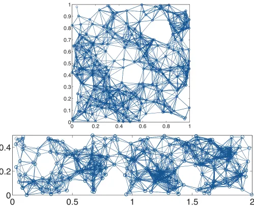
In Fig. 1 we illustrate two RRGs with dierent values of the rectangle side lengthaand the same number of nodes and edges. In the rst case whena= 1 the graph corresponds to the classical random geometric graph in which the
nodes are embedded into a unit square. The second case corresponds toa= 2and it represents a slightly elongated
rectangle.
A. About the connectivity of RRGs
An important question when studying RGGs in general is related to the connectivity of the resulting graphs. That is, for which values of the connection radius is an RGG withnnodes connected with high probability? In the case of the square, Penrose [35] proved that for the two-dimensional case
lim
n→∞P
¯
k−logn≤α= exp (−exp (−α)), (1)
whereP[· · ·] represents the probability that[· · ·] takes place and¯kis the average degree.
0 0.2 0.4 0.6 0.8 1 0
0.1 0.2 0.3 0.4 0.5 0.6 0.7 0.8 0.9 1
0
0.5
1
1.5
2
[image:4.612.56.555.52.459.2]0
0.2
0.4
Figure 1. Illustration of a RRG created with 250 nodes embedded into a unit square,a= 1, (top) and a unit rectangle with a= 2(bottom). In both cases the nodes are connected if they are at a Euclidean distance smaller or equal thanr= 0.15.
In the case of the RRG where the value ofk¯depends on the relation between the two sides of the rectangle we can
write (1) for the unit rectangle as [31]
lim
n→∞P[(n−1)f−logn≤α] = exp (−exp (−α)), (2)
wheref is given by
f =
0≤r≤a−1 πr2−4
3(a+a
−1)r3+1
2r 4,
a−1≤r≤a −4 3ar
3−r2a−2+1 6a
−4+ (4
3r 2+2
3a
−2)√a2r2−1
+2r2arcsin(1 ar), a≤r≤√a2+a−2 −r2(a2+a−2) +1
6(a
4+a−4)−1 2r
4
+(43r2a−1+2 3a)
√
r2−a2+ (4 3r
2+2 3a
−2)√a2r2−1
−2r2(arccos(ar1)−arcsin(ar)).
(3)
given by
¯
k= (n−1)f. (4)
Because the parameter α is unknown and it depends on the specic RRG considered, we have obtained a lower bound forexp (−exp (−α))using (2):
exp (−exp (−((n−1)f−logn)))≤exp (−exp (−α)). (5)
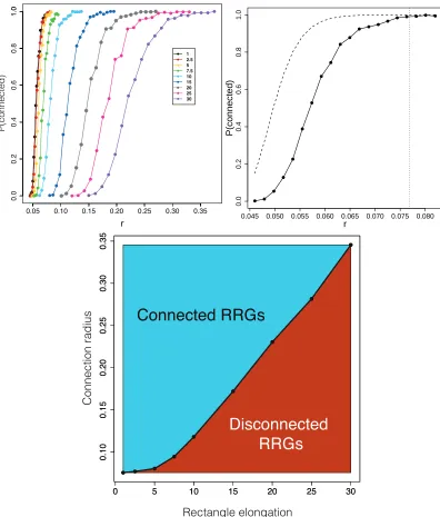
In Fig. 2 (a) we illustrate the variation of the connectivity of RRGs with the change of the connection radius for dierent values of the rectangle elongation obtained by computational realizations of the RRGs. As can be seen the probability that the RRG is connected changes as a sigmoid function with the increase of the connection radius in a similar way as in the case of the RGGs. However, as the elongation of the rectangle increases (increase of a) it is more dicult for the graph to be connected and the critical radius guaranteeing that the graph is connected increases signicantly with a. In panel (b) of Fig. 2 we illustrate the way in which we determine these critical radii. For a given value of a we nd the minimum value of r for which P(connected) = 1. Although we use in all cases the
values obtained from the simulations we can see that the theoretical bound forP(connected)(5) produce very similar
results.
We then plot the values of the connectivity radius versus the elongation of the rectangles (see Fig.2 (c)). The curve joining the points of this plot makes a separation between the RRGs which are connected (upper triangular part) from those which are disconnected (lower triangular part). That is, the curve represents the critical radii versus critical elongation, and it gives the critical region indicating the connectivity of the RRGs. It can be read in two dierent ways. You can x a value of a and then determine which is the critical radius for which the network will be disconnected. For instance, for a rectangle with longer sidea= 15 it is necessary to use radius larger than 0.17
to make the RRGs connected. More interesting for this work is the other way around. That is, we have a xed radius of connection, which may represent the radius of spreading of a disease among plants. Then, you can nd what elongation of the rectangle disconnects the network. For instance, if the connection radius is xed tor= 0.35every
RRG is connected for a < 30. Then, we emphasize here that we always work in the region of connected RRGs in
this work. That is, any analysis carried out in this paper is based on graphs for which the connectivity of the graph is 100% guaranteed as we work in the upper triangular part of this plot. In addition, we check computationally that every RRG generated in this work is connected.
III. EPIDEMICS ON NETWORKS
The spreading of an infectious disease on networks can be modeled representing individuals as nodes and the contacts between them as edges. In this context individuals are categorized in dierent compartments according to their health state [37]: i.e. susceptible (S) for individuals that can be infected by the disease, infected (I) for infectious individuals that can spread the pathogen or recovered (R) for individuals that already passed the disease and are immune to it.
Two fundamental models for disease spreading are the so-called SIS and SIR [37, 38]. The SIS is intended to model recurrent diseases that do not provide immunity, i.e. the common cold or most sexually transmitted diseases, where individuals can get the infection multiple times during their lifetime. Instead, in the SIR, once an individual get cured from the disease she enters the recovered compartment and cannot be infected again, that is, she acquires immunity. Both SIS and SIR dynamics are governed by two parameters, namely: the per contact infection rateβand the recovery rate µ. Let ,si,xi andri be the probabilities that the nodeiis susceptible, infected or has recovered from infection, respectively. The equations governing a SIS process are the following:
˙
si =−βsi
X
j
Aijxj+µxi, (6)
˙
xi =βsi
X
j
Aijxj−µxi, (7)
0.05 0.10 0.15 0.20 0.25 0.30 0.35 r 0 .0 0 .2 0 .4 0 .6 0 .8 1 .0 P(connected) 1 .0 1 2.5 5 7.5 10 15 20 25 30
0.045 0.050 0.055 0.060 0.065 0.070 0.075 0.080
0.0 0.2 0.4 0.6 0.8 1.0 r P(connected)
0 5 10 15 20 25 30
0 .1 0 0 .1 5 0 .2 0 0 .2 5 0 .3 0 0 .3 5
0 5 10 15 20 25 30
0 .1 0 0 .1 5 0 .2 0 0 .2 5 0 .3 0 0 .3 5 Rectangle elongation Connection radius
Connected RRGs
Disconnected
RRGs
Figure 2. (panel a) Change of the connectivity of RRGs with the change of the connection radius for dierent values of the rectangle elongation. (Panel b) Illustration of the way in which the critical radius for an RRG is obtained. Also the upper bound (5) (red dotted line) is illustrated. (Panel c) Plot of the critical versus the rectangle elongation for the RRGs. The line dividing the two regions represents the critical values of radius and elongation. All RRGs studied here have n= 1000nodes and all the calculations are the result of averaging 20 random realizations of the RRG with the given parameters.
˙
si=−βsi
X
j
Aijxj, (8)
˙
xi=βsi
X
j
Aijxj−µxi, (9)
˙
ri=µxi. (10)
[image:6.612.108.504.49.514.2]recovers from the disease. Note that the spreading of the disease depends on the network of contacts (an isolated individual can not catch the disease), while the recovery phase is independent of the substrate network (an isolated infected individual will recover after some time).
The ratioβ/µdrives the spreading of the disease. Depending on its infectious power two distinct phases are possible: an absorbing one where the spreading is not ecient enough to reach a large fraction of the system and the disease is absorbed and an active phase where the epidemics reaches a macroscopic fraction of the network. The transition from the absorbing to the active phase strictly resembles a non-equilibrium second order phase transition in statistical physics [39, 40]. The critical value of this transitionβ
µ
c
=τ is dened as the epidemic threshold. This term is also known as the basic reproduction number and it represents a threshold in the sense that whenτ <1the infection dies
out and ifτ >1the disease becomes an epidemic. In those cases whereτ= 1, the disease remains in the population
becoming endemic. The value of this threshold strongly depends on the topology of the network. In particular, for a given graphG= (V, E), it has been shown that [4143]:
τ = 1
λ1(G)
, (11)
where λ1(G) is the largest eigenvalue of the adjacency matrix of the network. In the case of RGG, Preciado and Jadbabaie [44] have made an exhaustive spectral analysis of virus spreading using the spectral moments of the adjacency matrix. They have found that for the RGG in d-dimensional cube, the spectral radius is bounded as λ1(G)< cdnrd, wherecd is a constant characteristic of the RGG in thed-dimensional cube. In 2-dimensional space this means that λ1(G) < c2nr2. Then, because in these graphs the average degree is nr2, the previous expression basically tells us that the spectral radius is bounded by the average degree of the RGG.
IV. EPIDEMIC THRESHOLD IN RRGS
In this section we concentrate more on the phenomenology of the process than in deriving analytical results about the dependance of the epidemic threshold with the topological parameters of the RRGs. Thus, we will obtain some sort of mean-eld approach that captures the behavior of the disease parameters with the topological ones. We start by considering the following well-known bounds for the largest eigenvalue of the adjacency matrix of a simple graph λ1(G) =λ1
¯
k≤λ1≤kmax, (12)
wherekmaxand¯kare the maximum and the average degree, respectively. Then, it is straightforward to realize that
τ≥ 1¯
k. (13)
Then, by replacing (4) into (13) we have the following bound for the epidemic threshold of a RRG
τ ≥ 1
(n−1)f. (14)
This result generalizes the one obtained by Preciado and Jadbabaie [44] for the RGG to the case where we have a rectangle of any elongation and where we consider explicitly the border eects of the rectangle (respectively the square in RGG).
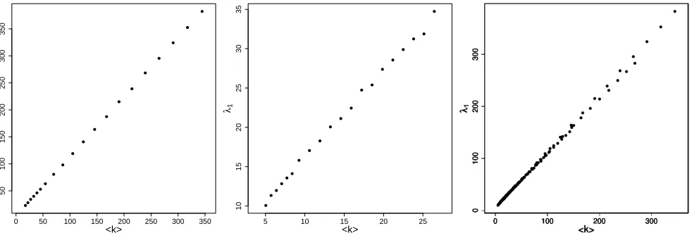
to the spectral radius of graphs in general. In particular, we are interested here in showing whether the average degree and the spectral radius of RRGs show the same behavior when the rectangle is elongated. In Figure 3 we illustrate the the plot of the spectral radius versus the average degree for RRGs with a = 1(left), a= 30 (centre)
anda= 1,2.5,5,7.7,15,20,25,30(right) for dierent values of the connection radius. As can be seen in all cases, and
particularly in the last one, the trend of the spectral radius and the average degree is exactly the same and indeed they are very highly linearly correlated. Thus, our conclusion here is that proving that the average degree have certain behavior when the rectangle is elongated can be directly extrapolated to the behavior of the spectral radius with the elongation of the rectangle.
0 50 100 150 200 250 300 350
50
100
150
200
250
300
350
<k>
λ1
5 10 15 20 25
10
15
20
25
30
35
<k>
[image:8.612.67.558.156.325.2]λ1
Figure 3. Scatter plots of the spectral radius versus the average degree for RRGs with a = 1 (left), a = 30 (centre) and a= 1,2.5,5,7.7,15,20,25,30(right) for dierent values of the connection radius.
Then, in order to prove this result we rst consider what happens to the functionf whena→ac. Let0< r≤a−1. Then, the rst derivative off1=f 0≤r≤a−1is given by
∂f1 ∂a =−
4 3r
3 1−a−2
, (15)
and since
1−a−2
≥0.
this is bounded by
∂f1 ∂a ≤0.
Leta−1≤r≤a. Then, the rst derivative off
2=f a−1≤r≤ais given by
∂f2 ∂a =
−4r3
3 +
2r2 a3 −
2 3a5 +
4(a4r4−2a2r2+ 1)
3a3√a2r2−1 (16)
which is bounded as,
∂f2
∂a ≤h <0, (17)
where
h= lim
r→a ∂f2
∂a =
2
a−
4a3
3 −
2 3a3 +
4(a8−2a4+ 1)
Leta≤r≤√a2+a−2. Then, the rst derivative off
3=f a≤r≤ √
a2+a−2
is given by
∂f3 ∂a = 2r
2
1
a3−a
+2 3
a3− 1 a5
+4(a
4r4−2a2r2+ 1)
3a3√a2r2−1 −
4(a4−2a2r2+r4)
3a2√r2−a2 , (19)
which is bounded as,
∂f2
∂a ≤g <0, (20)
where
g= lim
r→t ∂f3
∂a = 0. (21)
and t =√a2+a−2. Then, because all the derivatives are negative, we have proven the result. Strictly speaking the fact that1/(n−1)f increases with increasingadoes not necessarily imply thatτ will exhibit a similar trend for every a. However, as we will see in the next section there is a very good linear correlation between the values of τ obtained from the simulations and the lower bound1/(n−1)f , which indicates that both quantities follow the same trend as consequently that the previous assertion relating the behavior of the epidemic threshold when whena→ac is general. We discuss this in more detail in the net section.
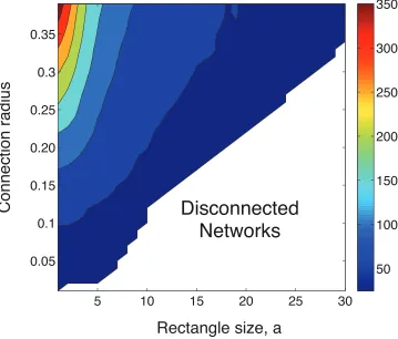
In the Fig. 4 we illustrate the plot of the spectral radius of the adjacency matrix of RRGs as a function of both the rectangle size lengthaand the connection radiusr. As expected the lower triangular part of the plot corresponds to the disconnected RRGs, which are never used in this work. However, in the upper triangular part of the plot we observe a large variation of the spectral radius λ1 of an RRG with both parameters of the model. For a xed connection radius the values ofλ1decay with the elongation of the rectangle as expected from the previous analytical results. Notice thatλ1can change as much as from380to35for a constant radiusr= 0.4when changing the rectangle size froma= 1toa= 30. This, of course, is the main cause of the change of the epidemic threshold predicted by the
bound (13) obtained at the beginning of this section.
V. EPIDEMICS ON RRGS. SIMULATIONS
In this section we conduct extensive numerical simulations of the SIS dynamics for dierent values of the elongation aand xed radiusr with the goal of checking the goodness of the bound dened in Eq. 13 and to illustrate how the elongation of the rectangle in the RRG model changes the epidemic dynamics. In the simulations we start seeding the infection in a small fraction ρ0 = 0.01 of the nodes and let the SIS dynamics evolve for 5·104 time-steps. At this point, we let the simulations run for an additional 103 time-steps and calculate the fraction of infected nodesρ as the average ofρ(t)over this period. For each selection of the parameters we performed250 independent runs with
[image:9.612.69.555.76.241.2]dierent initial conditions. The nal value ofρis obtained as the average over all the runs.
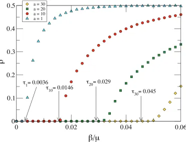
Figure 5 shows the fraction of infected nodes in the stationary state against the infection rateβ for dierent values ofa= 1,10,20,30. The values shown by arrow are the analytical ones obtained using (14).
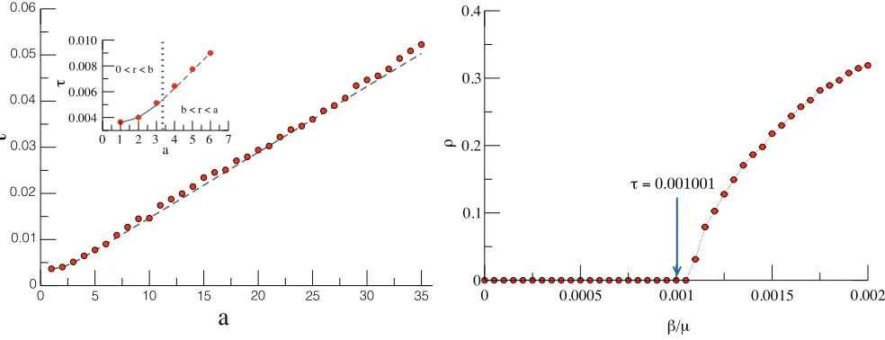
To have a more detailed picture of the behavior of the epidemic threshold, in Fig. (6a) we compare the theoretical bound with the epidemic threshold obtained via the numerical simulations. As we have stressed in the previous section this comparison is very important for understanding whether the epidemic threshold and the bound1/(n−1)f follow the same trend with the elongation of the rectangle. Our comparison covers two of the three cases of Eq. 3: 0≤r≤a−1 anda−1 ≤r≤arespectively. As can be seen in this Figure the lower bound 14 is very tight, and more importantly the bound and the 'observed' epidemic threshold display the same behavior when the rectangle elongation change. Indeed, our analysis of the dierence between the observed value of the epidemic threshold and the lower bound obtained by Eq. 13 shows that for all the RRGs having1 ≤a≤35such relative dierence is 2.93% and in no case
it is larger than 10%. Also we observe no trend in the relative dierence related to the elongation of the rectangle. That is, the relative dierence is neither increasing nor decreasing with the elongation of the rectangle.
Rectangle size, a
C
o
n
n
e
ct
io
n
ra
d
iu
s
5
10
15
20
25
30
0.05
0.1
0.15
0.20
0.25
0.3
0.35
50
100
150
200
250
300
350
[image:10.612.136.495.76.382.2]Disconnected
Networks
Figure 4. Values of the spectral radiusλ1 of the adjacency matrix of RRGs withn= 1000nodes as a function of the rectangle
size lengthaand the connection radiusr. The bottom-right part of the plot corresponds to networks which are created with
radius below the critical radius,r < rc(see plot (c) in Fig. 2), and consequently are disconnected. All the calculations are the
result of averaging 20 random generations of the RRG with the given parameters.
In the case of disease propagating on plants, these resultsboth analytical and simulationscoincide with the eld observations and simulations using stochastic models [2230] which suggest that square plots and elds favored higher spreading of plant diseases than elongated ones of the same area [2225].
Our analytical and simulation results point to the fact that under the same conditions, the propagation of an epidemic on a rectangular plot/eld is much harder than on a square one because a larger number of infected individuals is needed for the disease to become epidemic. Here we have kept the size of the plot/eld constant by considering unit rectangles in our analysis. However, it is important to consider that other factors, such as the orientation of the plot/eld play fundamental role in the propagation of a disease on plants. For instance, if the rectangular plots are placed perpendicular to the direction of the prevalent winds the disease will not propagate as a consequence of this factor.
VI. CONCLUSIONS
0
0.02
0.04
0.06
β/μ
0
0.1
0.2
0.3
0.4
0.5
ρ
a = 30 a = 20 a = 10 a = 1
τ
10= 0.0146
τ
20= 0.029
τ
30= 0.045
τ
1= 0.0036
Figure 5. (a) Fraction of infected nodes at the stationary state ρas a function of the infection rateβ for dierent values of a= 1,10,20,30.a= 1represents the rst case (0≤r≤a−1) of Eq. 3 whilea= 10,20,30fall in the second case (a−1≤r≤a).
Other parameters are: n= 103 nodes,r= 0.35andµ= 1.0. Each point is an average over250independent runs. The values shown by arrow are the analytical ones obtained using (14).
These results agree with a large accumulation of empirical evidence about the role of plots/elds elongation on the propagation of diseases on plants. This model represents a new way to analyze disease propagation on plants or similar scenarios, by combining the heterogeneities introduced at individual level by networks with the inuence produced by the shape variation of the plots and elds where the plants are growing.
ACKNOWLEDGMENTS
[image:11.612.126.497.51.335.2]0 5 10 15 20 25 30 35
a
0 0.01 0.02 0.03 0.04 0.05 0.06
τ
0 1 2 3 4 5 6 7a
0.004 0.006 0.008 0.010
τ
0 < r < b
b < r < a
0 0.0005 0.001 0.0015 0.002
β/μ
0 0.1 0.2 0.3 0.4
ρ
τ = 0.001001
Figure 6. (panel a) Comparison between the theoretical bound and the epidemic threshold obtained via numerical simulations. Line represents the theoretical prediction of Eq. 13 while points represent the numerical threshold. The inset shows a zoom for the rst case of Eq. 30≤r≤a−1 (full line) and the second casea−1 ≤r≤a(dashed line). Other parameters are: n= 103 nodes, r= 0.35and µ= 1.0. Each point is average over 250independent runs. (panel b) Fraction of infected nodes at the steady stateρ as a function of the infection rateβ for a≤r ≤ √a2+a−2. In the simulationsa = 3and r = 3.01. Other
parameters are: n= 103nodes andµ= 1.0. Each point is average over250independent runs.
[1] Boccaletti, S., Latora, V., Moreno, Y., Chavez, M., & Hwang, D. U. (2006). Complex networks: Structure and dynamics. Phys. Rep., 424(4), 175-308.
[2] Boguã, M., Pastor-Satorras, R., & Vespignani, A. (2003). Absence of epidemic threshold in scale-free networks with degree correlations. Phys. Rev. Lett., 90(2), 028701.
[3] Castellano, C., & Pastor-Satorras, R. (2010). Thresholds for epidemic spreading in networks. Phys. Rev. Lett., 105(21), 218701.
[4] Jeger, M. J., Pautasso, M., Holdenrieder, O., & Shaw, M. W. (2007). Modelling disease spread and control in networks: implications for plant sciences. New Phytologist, 174(2), 279-297.
[5] Handford, T. P., Pérez-Reche, F. J., Taraskin, S. N., Costa, L. d. F., Miazaki, M., Neri, F. M., Gilligan, C. A. (2011). Epidemics in networks of spatially correlated three-dimensional root-branching structures. J. Roy. Soc. Interface, 8 , 423-434.
[6] Neri, F.M., Bates, A., Füchtbauer, W.S., Pérez-Reche, F.J., Taraskin, S.N., Otten, W., Bailey, D.J. and Gilligan, C.A. (2011). The eect of heterogeneity on invasion in spatial epidemics: from theory to experimental evidence in a model system. PLOS Comput Biol, 7(9), p.e1002174.
[7] Neri, F.M., Pérez-Reche, F.J., Taraskin, S.N. and Gilligan, C.A. (2010). Heterogeneity in susceptibleinfectedremoved (SIR) epidemics on lattices. Journal of The Royal Society Interface, p.rsif20100325.
[8] Pérez-Reche, F.J., Taraskin, S.N., Costa, L.D.F., Neri, F.M. and Gilligan, C.A. (2010). Complexity and anisotropy in host morphology make populations less susceptible to epidemic outbreaks. Journal of the Royal Society Interface, 7(48), pp.1083-1092.
[9] Penrose, M. (2003). Random geometric graphs (Vol. 5). Oxford: Oxford University Press. [10] Dall, J., & Christensen, M. (2002). Random geometric graphs. Phys. Rev. E, 66(1), 016121. [11] Bollobas, B. (1985). Random graphs. Academic Press: New York.
[12] Gilbert, E. N. (1959). Random graphs. Ann. Math. Stat., 30(4), 1141-1144.
[13] Wang, P., & González, M. C. (2009). Understanding spatial connectivity of individuals with non-uniform population density. Trans. Royal Soc. A: Math., Phys. Eng. Sci., 367(1901), 3321-3329.
[14] Díaz-Guilera, A., Gómez-Gardeñes, J., Moreno, Y., & Nekovee, M. (2009). Synchronization in random geometric graphs. Int. J. Bif. Chaos, 19(02), 687-693.
[15] Nekovee, M. (2007). Worm epidemics in wireless ad hoc networks. New J. Phys., 9(6), 189.
[16] Isham, V., Kaczmarska, J., & Nekovee, M. (2011). Spread of information and infection on nite random networks. Phys. Rev. E, 83(4), 046128.
[17] Toroczkai, Z., & Guclu, H. (2007). Proximity networks and epidemics. Physica A, 378(1), 68-75.
[image:12.612.66.558.52.241.2][19] Riley, S., Eames, K., Isham, V., Mollison, D., & Trapman, P. (2015). Five challenges for spatial epidemic models. Epidemics, 10, 68-71.
[20] Zhang, W., Lim, C. C., Korniss, G., & Szymanski, B. K. (2014). Opinion dynamics and inuencing on random geometric graphs. Sci. Rep., 4, 5568.
[21] Brooks, C. P., Antonovics, J., & Keitt, T. H. (2008). Spatial and temporal heterogeneity explain disease dynamics in a spatially explicit network model. Am. Nat., 172(2), 149-159.
[22] Paysour, R. E., & Fry, W. E. (1983). Interplot interference: A model for planning eld experiments with aerially dissemi-nated pathogens. Phytopathology, 73(7), 1014-1020.
[23] Waggoner, P. E. (1962), Weather, space, time, and chance of infection. Phytopathology. 52(11), 11001108.
[24] James, W. C., & Shih, C. S. (1973). Size and shape of plots for estimating yield losses from cereal foliage diseases. Expl. Agric., 9(01), 63-71.
[25] Fleming, R. A., Marsh, L. M., & Tuckwell, H. C. (1982). Eect of eld geometry on the spread of crop disease. Protection Ecology (Netherlands) 4, 81108.
[26] Bonnot, F., De Franqueville, H., & Lourenço, E. (2010). Spatial and spatiotemporal pattern analysis of coconut lethal yellowing in Mozambique. Phytopathology, 100(4), 300-312.
[27] Mundt, C. C., Brophy, L. S., & Kolar, S. C. (1996). Eect of genotype unit number and spatial arrangement on severity of yellow rust in wheat cultivar mixtures. Plant Pathology, 45(2), 215-222.
[28] Mundt, C. C., & Brophy, L. S. (1988). Inuence of number of host genotype units on the eectiveness of host mixtures for disease control: a modeling approach. Phytopathology. 78, 108794.
[29] Xu, X. M., & Ridout, M. S. (2000). Eects of quadrat size and shape, initial epidemic conditions, and spore dispersal gradient on spatial statistics of plant disease epidemics. Phytopathology, 90(7), 738-750.
[30] Ferrandino, F. J. (2005). The explicit dependence of quadrat variance on the ratio of clump size to quadrat size. Phy-topathology, 95(5), 452-462.
[31] Estrada, E., & Sheerin, M. (2015). Random rectangular graphs. Phys. Rev. E, 91(4), 042805.
[32] Coon, J., Dettmann, C. P., & Georgiou, O. (2012). Full connectivity: corners, edges and faces. J. Stat. Phys., 147(4), 758-778.
[33] Coon, J. P., Georgiou, O., & Dettmann, C. P. (2014, May). Connectivity in dense networks conned within right prisms. In Modeling and Optimization in Mobile, Ad Hoc, and Wireless Networks (WiOpt), 2014 12th International Symposium on (pp. 628-635). IEEE.
[34] Dettmann, C. P., Georgiou, O., & Coon, J. P. (2014). More is less: Connectivity in fractal regions. arXiv preprint arXiv:1409.7520.
[35] Penrose, M. D. (1997). The longest edge of the random minimal spanning tree. Ann. Appl. Prob., 340-361.
[36] Coon, J., Dettmann, C. P., & Georgiou, O. (2012). Impact of boundaries on fully connected random geometric networks. Phys. Rev. E, 85(1), 011138.
[37] Bailey, N. T. (1975). The mathematical theory of infectious diseases and its applications. Hafner Press.
[38] Anderson, R. M., May, R. M., & Anderson, B. (1992). Infectious diseases of humans: dynamics and control (Vol. 28). Oxford: Oxford university press.
[39] Marro, J., & Dickman, R. (1999). Nonequilibrium phase transitions in lattice models. Cambridge University Press. [40] Henkel, M., Hinrichsen, H., Lübeck, S., & Pleimling, M. (2008). Non-equilibrium phase transitions (Vol. 1). Berlin: Springer. [41] Chakrabarti, D., Wang, Y., Wang, C., Leskovec, J., & Faloutsos, C. (2008). Epidemic thresholds in real networks. ACM
Transactions on Information and System Security (TISSEC), 10(4), 1.
[42] Gómez, S., Arenas, A., Borge-Holthoefer, J., Meloni, S., & Moreno, Y. (2010). Discrete-time Markov chain approach to contact-based disease spreading in complex networks. Europhys. Lett., 89, 38009.
[43] Van Mieghem, P., Omic, J., & Kooij, R. (2009). Virus spread in networks. Networking, IEEE/ACM Transactions on, 17(1), 1-14.