A General Procedure for Constructing Mortality Models

City, University of London Institutional Repository

Citation

:

10.1080/10920277.2013.852963

This is the accepted version of the paper.

This version of the publication may differ from the final published

version.

Permanent repository link:

Link to published version

:

Copyright and reuse:

City Research Online aims to make research

outputs of City, University of London available to a wider audience.

Copyright and Moral Rights remain with the author(s) and/or copyright

holders. URLs from City Research Online may be freely distributed and

linked to.

City Research Online: http://openaccess.city.ac.uk/ [email protected]

DISCUSSION PAPER PI-1301

A General Procedure for Constructing

Mortality Models

Andrew Hunt and David Blake

January 2015

ISSN 1367-580X

The Pensions Institute

Cass Business School

City University London

106 Bunhill Row

London EC1Y 8TZ

UNITED KINGDOM

A General Procedure for Constructing

Mortality Models

Andrew Hunt

Cass Business School, City University London

Corresponding author: [email protected]

David Blake

Pensions Institute, Cass Business School, City University London

Amended 20 January 2015

Abstract

Recently, a large number of new mortality models have been pro-posed to analyse historical mortality rates and project them into the future. Many of these suffer from being over-parametrised or have terms added in an ad hoc manner which cannot be justified in terms of demographic significance. In addition, poor specification of a model can lead to period effects in the data being wrongly attributed to co-hort effects which results in the model making implausible projections. We present a general procedure for constructing mortality models us-ing a combination of a toolkit of functions and expert judgement. By following the general procedure, it is possible to identify sequentially every significant demographic feature in the data and give it a para-metric structural form. We demonstrate using UK mortality data that the general procedure produces a relatively parsimonious model that nevertheless has a good fit to the data.

∗_{We are grateful to participants at a seminar at Cass Business School, at the Longevity}

8 conference in Waterloo, Canada, in 2012, at the Perspectives on Actuarial Risks in Talks of Young Researchers winter school in Ascona, Switzerland, in 2013, and to the anonymous referee for comments received which have improved this paper. We are also grateful to Andr´es Villegas for many useful discussions.

Keywords: Mortality modelling, age/period/cohort models, age pe-riod effects, cohort effects

1

Introduction

In recent years, there has been an explosion in the number of new mortal-ity models that have been proposed. This has been triggered, in part, by the greater focus placed on longevity risk by demographers, actuaries and governments. It has also been prompted by the failure of existing models to identify adequately the full extent of the complexities involved in the evolu-tion of mortality rates over time.

Yet these new models often involve ad hoc extensions to existing mod-els, which have questionable demographic significance.1 Despite having more terms than the older models, they still fail to capture a lot of the information present in the data, such as the level of lifespan inequality in the population. They also have difficulties providing realistic forecasts of specific mortality rates. Lacking a formal procedure for interrogating the data to establish what structure remains to be explained, modellers too often add new terms based on theoretical models of mortality or on assumptions regarding the shape of the mortality curve rather than evidence. This is especially dan-gerous in models with cohort parameters intended to capture generational effects. The result of any mis-specification in these extra age/period terms can result in structure being wrongly attributed to the cohort effect. This is then projected incorrectly, moving up the age range with the passage to time, with the result that implausible forecasts are generated at higher ages.

In view of this, we feel that the time has come to take a fresh look at mortality model construction. But, rather than propose yet another new model, what we do in this paper is outline and implement a “general proce-dure” (GP) for building a mortality model from scratch, driven by a forensic examination of the data. Through an iterative process, the GP identifies every significant demographic feature in the data in a sequence, beginning

1

Demographic significance is defined in Hunt and Blake (2015e) as the interpretation of the components of a model in terms of the underlying biological, medical or socio-economic causes of changes in mortality rates which generate them.

with the most important. For each demographic feature, we need to apply expert judgement to choose a particular parametric form to represent it. To do this, we need a “toolkit” of suitable functions.

By following the GP, it is possible to construct mortality models with suf-ficient terms to capture accurately all the significant information present in the age, period and cohort dimensions of the data. In particular, the GP pre-vents structure in the data which is genuinely associated with an age/period effect being wrongly allocated to a cohort effect. The procedure is general in the sense that it can be applied to any dataset to give a fully specified model tailored to the features of the population under consideration. Most signifi-cantly, the GP provides evidence for the addition of each term to an existing model; it allows each new term to be associated with a specific demographic and biological process driving the evolution of mortality rates.

Section 2 presents a summary of the structure of the class of mortal-ity models we are considering and sets out the desirable properties that we believe a good mortality model should possess. The general procedure is discussed in Section 3. In Section 4, we apply the GP to data for men in the UK and describe how the steps in Section 3 operate in practice. In Section 5, we assess the goodness of fit of this model and check whether there is any remaining structure present in the fitted residuals. Section 6 compares the GP with the Lee-Carter model and with a procedure based on principal com-ponent analysis as an alternative method of constructing mortality models with multiple age/period terms. Finally, Section 7 concludes with an assess-ment of how the final model found measures up against our set of desirable properties from Section 2 as well as its advantages and disadvantages.

2

The structural form of mortality models

The majority of existing mortality models proposed in the actuarial literature fall into an age/period/cohort framework. This transforms the observed mortality rates and then fits a series of terms to account for the interactions between the age,x, the year of observation,t, and the year of birth,y=t−x, for the population within each cell of data. Mathematically, this can be

written as:2

η

E

Dx,t

Ex,t

=αx+ N

X

i=1

f(i)(x;θ(i))κ(i)_t +γt−x (1)

This equation has the following components:

• a link function η to transform the observed data into a form suitable for modelling. The raw data usually consists of death counts Dx,t and

exposures to risk Ex,t at agesx and for years t;

• a static age function αx to capture the general shape of the mortality

curve that does not change with time;

• N age/period terms f(i)(x;θ(i))κ(i)_t , consisting of companion pairs of period terms κ(i)_t (or “trends”) which give the evolution of mortality rates through time and age functionsf(i)_(x;θ(i)_{) which determine which}

segments of the age range these trends affect; and

• cohort parameters γt−x which determine the lifelong effects that are

specific to different generations as discussed in Willets (2004), denoted by their year of birth;

Many mortality models proposed to date can be written in this form. These include the Lee-Carter (LC) model proposed in Lee and Carter (1992) and extensions of this, such as those of Renshaw and Haberman (2003) and Yang et al. (2010). It also includes the Cairns-Blake-Dowd family of mortality models (in Cairns et al. (2006a) and Cairns et al. (2009)), the classic age/period/cohort model of Hobcraft et al. (1982) and developments of these models such as the models proposed by Plat (2009) and O’Hare and Li (2012). In addition, it includes various other mortality models not contained within these families such as the ones proposed in Wilmoth (1990) and Aro and Pennanen (2011). The models of the rate of mortality change proposed in Haberman and Renshaw (2012, 2013) and Mitchell et al. (2013) also fall within this structure for suit-able choice of the link function ηx,t. These models and the relationships

between them are discussed in greater depth in Hunt and Blake (2015e). 2

This structural form and demographic significance of the terms in it are discussed in depth in Hunt and Blake (2015e).

Examples of models which fall outside this framework include those with a constant, Makeham term, the extension to the LC model proposed in Renshaw and Haberman (2006) (due to the presence of the βx(0) term

modi-fying the cohort parameters) and the P-splines models of Currie et al. (2004).

A good mortality model should satisfy the following “desirability criteria”: 1. provide an adequate fit to the data, with sufficient terms to capture all

the significant structure in the data;

2. be biologically reasonable;3 _{and have terms which have demographic}

significance in the sense that they are explainable in terms of the un-derlying biological, medical or socio-economic causes of changes in mor-tality rates at specific ages

3. be parsimonious, with the smallest number of terms needed to capture this structure, and with each term using as few parameters as possible; 4. be robust, in that parameter uncertainty should be low and small changes in the data should not result in significant changes in the esti-mates of the parameters and in our interpretation of them;

5. span the full age range, with sufficient terms to model the complex shape of and dynamics observed in mortality rates at younger ages; and

6. include cohort effects if justified by the data and allow for these to be clearly distinguished from age/period effects to allow plausible projec-tions of the model.

The GP has been designed with these criteria (and the trade-offs between them) in mind. Most specifically, the GP chooses parametric age functions,4

f(i)(x;θ(i)), which take a specific functional form and are parameterised by a small number of variables θ(i), over more general non-parametric age func-tions,5 _β(i)

x , due to their parsimony and because we can use our judgement

3

Introduced in Cairns et al. (2006b) and defined as “a method of reasoning used to establish a causal association (or relationship) between two factors that is consistent with existing medical knowledge”.

4

Defined in Hunt and Blake (2015e) as one taking a specific functional form that is defined by an algebraic formula

5

Defined in Hunt and Blake (2015e) as one fitted without imposing any a priori struc-ture across ages

to assign demographic significance to the term in question. The advantages and disadvantages of using parametric age functions are discussed in greater depth in Hunt and Blake (2015e). However, a key feature of the GP is to use the information discovered from first using a non-parametric age function to provide guidance on the shape of that demographic feature. This will im-prove the goodness of fit for each term and avoid the need to make a priori assumptions regarding which age functions to use.

3

A general procedure for constructing

mor-tality models

The general procedure consists of the following steps:

1. Start with a static age function αx to capture the time-independent

shape of the mortality curve across ages in the data set under consid-eration;

2. Add a companion pair of non-parametric age and period functionsβxκt

to find the most significant age/period effect not captured by the model so far, where the age term βx is free to take the shape that maximises

the fit to the data;

3. Observe the shape of the estimated age term βx across ages and how

κt has evolved through time;

4. Check that the addition of the new pair of terms improves the overall goodness of fit to the data;

5. Use judgement to select a specific smooth functional form f(x;θ) to replace the non-parametric age term βx where the function is defined

by a small number of free parameters θ;

6. Check whether the fitted model with this specific functional form

(a) a) produces a similar evolution over time as the non-parametric term by comparing the fitted κt’s for the two cases and

(b) b) achieves comparable improvements in the goodness of fit as the non-parametric term.

7. Check whether the addition of the new companion pair of terms has significantly changed the shape of previously selected terms, in which case we might need to change and re-estimate the earlier terms;

8. Repeat steps 2 to 7 until we are satisfied that the model captures all significant age and period structure in the data;

9. Add a cohort term γt−x to capture any year of birth effects;

10. Test the final model for goodness of fit and robustness, and the residuals for the properties of normality and independence, thereby confirming that there is no significant unexplained demographic structure remain-ing in the data;

11. Compare the final model to alternative models estimated using the same data set.

After each modification of the model structure (e.g., replacing a non-parametric age function, βx, with a parametric alternative, f(x), or the addition of the

cohort term), all the terms are re-estimated by fitting the model to historical data.6 _{This ensures that all of the parameters are estimated on the basis of}

maximising the fit to data and that there is no explicit hierarchy within the model structure. Figure 1 shows a flow chart of the GP summarising these steps.

The GP is a data-driven procedure, with terms being selected based on their ability to capture features of the observed mortality rates. At high level, it is a specific-to-general model building procedure (as defined in Campos et al. (2005)) as it begins with a simple model and sequentially adds terms in order to build a model that fully reflects the features contained in the dataset under investigation. This approach is unavoidable, as to begin with a fully general mortality model, as required by the general-to-specific methodology, would contain such a large number of terms that it would be impossible to fit it to data and difficult to simplify. However, at the “mi-cro” level, each age/period companion pair is added in a general-to-specific fashion - the most general form of the function is added to the model and then simplified into a specific, parametric form, whilst seeking to retain its

6

The only exception to this is when an exploratoryβxκt term is added to the model,

since these models are often very unstable due to over-parametrisation.

Start with static life table -αx

Add non-parametric

term -βxκt Refit model Observe

Check improves fit

Find paramet-ric form -f(x)κt

Yes

Refit model Test trends Same trend?

Test goodness of fit

No Yes

More AP terms needed?

Yes

Add cohort term -γy

No

No

Refit model Test goodness of fit Model adequate?

Final model

Yes

No

Figure 1: Flow chart of the general procedure

explanatory power. Thus, we believe that the GP benefits from both model-building frameworks.

The GP selects the functional form of the age/period terms in two stages. First, it allows each age/period term within the data to be identified by a non-parametric age function without requiring any a priori assumptions to be made by the modeller. Second, it allows the shape of these non-parametric age functions to guide the choice of parametric function that is selected from the toolkit to match as closely as possible the explanatory power of the for-mer, whilst benefiting from parsimony in terms of the number of parameters to be estimated. However, judgement is required in the selection of the parametric function, although that the GP provides evidence to justify the decision made.

Appendix A gives details of the “toolkit” of parametric age functions needed to implement the GP; it also gives a general algorithm for estimating the free parameters in them. However, a toolkit is never complete and so we do not offer this as an exhaustive list of functions - only as those we have considered so far. Two highly desirable features for a function to be included in the toolkit are a small number of free parameters (in our experience, more than two free parameters leads to unstable estimates) and the ability to ad-just the location of the function in the age range.

At each stage of the GP, we need to assess whether the resulting model is in accordance with our desirability criteria. First, we will need to test whether an additional age function improves the fit of the model to data. It is well known that a measure such as the log-likelihood will always show an improvement in the fit of a series of nested models to the data due to the increased number of free parameters. In order to achieve our desire for a parsimonious model, it is therefore necessary to penalise the number of free parameters used by considering a measure such as the Bayes Informa-tion Criterion (BIC).7_{The log-likelihood is still useful, however, when adding}

an additional non-parametric term as the change in this measure represents the maximum possible improvement in the fit from the addition of a single new term. We can therefore use this maximum possible improvement as the benchmark for measuring the success of the specific parametric form being

7

Defined asmax(Log-likelihood)−0.5× No. free parameters ×ln(No. data points).

trialled: a parametric age function which produces 80-90% of the same im-provement in log-likelihood can be regarded as highly desirable.

Second, we need to compare whether the structure identified by a non-parametric age function is the same as that found when a specific non-parametric function is introduced. Plots of the two are useful for revealing the general pattern of mortality change and identifying features such as trend changes and outliers that the two series have in common.

Finally, we will need to test the residuals from the data. As discussed in Pitacco et al. (2009), under a Poisson model for deaths (such as the one we use), the standardised deviance residuals rx,t are given by

rx,t =sign(dx,t−dˆx,t)

v u u t

2Wx,t

φ dx,tln dx,t

ˆ dx,t

!

−(dx,t−dˆx,t)

!

with actual death count dx,t, fitted death count ˆdx,t = Ex,tc µx,t, and φ the

scale parameter given by the total fitted deviance divided by the number of degrees of freedom8 _{of the model. This assumes that the residuals have}

con-stant variance across age and time. For large expected death counts, these should be approximately standard normal variables, so we can test the resid-uals for normality using the Jarque-Bera test of the skewness and kurtosis to check this. The residuals should also be independent and show no obvi-ous structure across ages, periods and cohorts. To look for structure within the residuals, we plot heat maps and visually inspect for obvious vertical, horizontal or diagonal banding patterns. This would indicate the presence of further age, period or cohort effects. We also calculate the correlations of the residuals with their neighbours in the age and period directions, and test these correlations against the assumption of independence.

To exit the cycle of adding new age/period terms, we need a stopping rule in the GP to determine when there are no further demographically sig-nificant age/period terms left unidentified in the data. Such a stopping rule will inevitably be subjective. This means that the GP is not a “black-box” algorithm; it requires the active engagement and exercise of judgement by

8

Number of data points less number of free parameters.

the modeller at each stage of the model building process.

Finally, we add the cohort parameters as the last step in the GP. The reason for this reflects a preference for a model where the majority of the temporal dependence in the data is allocated to the age/period terms. The reasons for this preference are discussed in detail in Hunt and Blake (2015e), but in our experience, the pattern of fitted cohort parameters produced by some models does not seem to have any demographic significance and may be caused by the model trying to compensate for inadequate age/period terms. We therefore seek to avoid this in the GP.

4

Application of procedure to male UK data

To illustrate the GP, we apply it to data for men in the UK from 1950 to 2009 covering ages 0 to 100 (ungrouped) downloaded from the Human Mor-tality Database (Human MorMor-tality Database (2014)). We restrict the data to the period since the Second World War as it is free from major conflicts and abrupt social upheaval. Since the Human Mortality Database provides central exposures to risk for each age and year, we assume that the death counts are Poisson random variables and therefore use a log-link function for ηx,t as it is the canonical link function for the Poisson distribution, as

discussed in Hunt and Blake (2015e). We fit the model at each stage using Poisson maximum likelihood estimation using the algorithms described in Appendix A.

4.1

Stage 0 - Static life table

The static life table produced by fitting ln(µx,t) = αx constitutes the first

step in the GP. The fitted values of αx (not shown) show the usual pattern

of mortality across the full age range: with high mortality rates at age zero due to infant mortality, the log-linear pattern of mortality increases at high ages (from 50 to 90) and the increased rates of mortality due to the accident hump between ages 15 and 25. Whilst the age function is refitted at each stage of the GP, this shape does not change significantly throughout the different stages of the model building process.

4.2

Stage 1 - First age/period term

The next step is to add the first non-parametric age/period term to the static model to arrive at ln(µx,t) =αx+βxκ(1)t , which has the form of the LC model.

This gives the familiar βx and κ(1)t terms shown in Figure 2.

In order to fully identify the model, we impose

X

x

|βx|= 1 (2)

X

t

κ(1)_t = 0 (3)

and adopt these identifiability constraints for all subsequent age/period terms in the model for consistency. For parametric age functions, imposing Equa-tion 2 involves rescaling the age funcEqua-tion by either a constant or with a func-tion of the free parameters, θ(i) (i.e., ensuring that the age function is “self-normalising”). This is discussed further in Appendix A and Hunt and Blake (2015b).

In the interests of parsimony and demographic significance, we believe that it is highly desirable to find a simpler parametric form than the age function of the LC model to capture the impact of the dominant trend within the data - ideally the simplest age function that will capture the same trend. This parametric form should be continuous to avoid any issues with the smoothness of projected mortality rates. As the fitted βx age

func-tion is positive across the whole age range, it might be felt to represent a general improvement in mortality rates across all ages. Appealing to this demographic significance, we therefore try the simplest possible age function - a constant. As Figure 2 shows, this simple age function effectively captures the same trend as the non-parametricβxfunction with 100 fewer parameters,

and achieves approximately 92% of the same improvement in log-likelihood. We are therefore satisfied that there is no need to use a more complex and less parsimonious age function, although we would expect that much of the age structure present in the fitted βx will need to be captured by subsequent

age/period terms.

Figures 2a and 2b shows the age and period functions generated by Stage 1 of the GP. We can see that the population has experienced sustained

0 20 40 60 80 100 0

0.005 0.01 0.015 0.02 0.025 0.03

Age

β_x f(x)

(a) Age functions

1950 1960 1970 1980 1990 2000 2010 −80

−60 −40 −20 0 20 40

Year Corr = 1.00

Non−Parametric Parametric

(b) Period functions

Figure 2: Age and period functions for Stage 1 of the general procedure

provements in mortality which have accelerated slightly in recent years. The model also detects the increased mortality in 1951 owing to the influenza epidemic in that year which affected much of England.

So far, so good, but a plot of the residuals - not shown here - indicates that additional terms are necessary to fully capture all the structure within the data.

4.3

Stage 2 - Second age/period term

In order to find the next most significant age/period effect within the data, we now add another non-parametric age/period term to the model to arrive at

ln(µx,t) =αx+f(1)(x)κ(1)t +βxκ(2)t (4)

The fitted model gives the values of βx and κ(2)t shown in Figure 3. It

is not a trivial task to select an appropriate parametric age function from the shape of βx and this is where judgement becomes important. By

in-spection, the non-parametric age function appears to have two components - an upward-sloping linear trend across the entire age range and a large “hump” superimposed on the age range 10 to 50. Since we can assign differ-ent demographic significance to each of these features, it is appropriate that we separate them into two different age/period terms in the fully specified model. However, these trends will probably be highly correlated which is why the non-parametric function has combined them.

We choose to fit a straight line as our choice off(2)(x) as it is a simpler potential function than one with a hump shape; indeed it is the simplest possible function after a constant. In our experience, a straight line is often the second choice of age function that arises naturally when applying the GP, especially for data restricted to higher ages. This lends support for the use of the Cairns-Blake-Dowd class of models. A straight line can be inter-preted as determining changes in the slope parameter in a Gompertz model of mortality for models with a logarithmic link function. This is related to the “rectangularisation” of the mortality curve, as a greater proportion of deaths at high age occur around the median age of death. We also note that κ(1)_t and κ(2)_t are negatively correlated, consistent with the Strehler-Mildvan

law of mortality discussed in Finkelstein (2012).

4.4

Stage 3 - Third age/period term

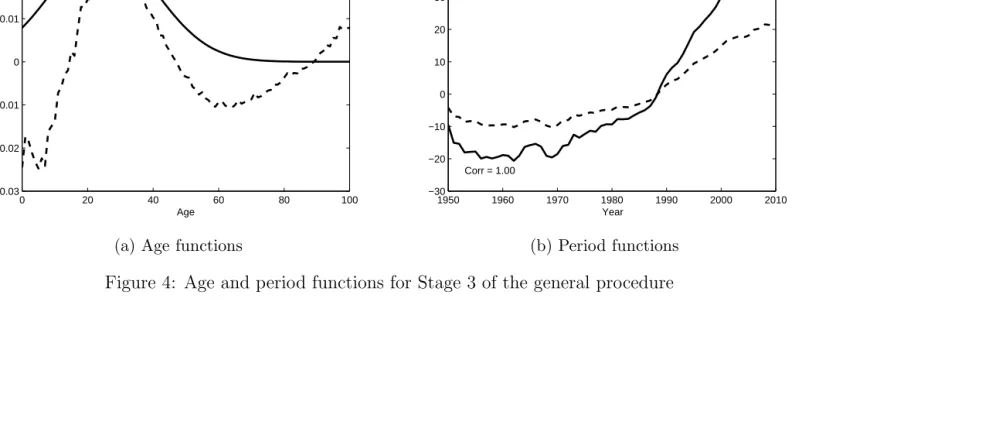
Our discussion of the choice of an appropriate age function at Stage 2 should give us a strong idea as to the appropriate shape of the age function for Stage 3. The GP gives us the evidence to support or reject our conjecture by first extending the model with a new non-parametric age/period term

ln(µx,t) =αx+ 2

X

i=1

f(i)(x)κ(i)_t +βxκ (3)

t (5)

The fitted non-parametric model gives the values of βx and κ(3)t shown

in Figure 4. This confirms that a suitable choice for f(3)_{(x) could indeed}

be some form of hump-shaped function centred around age 25 and so we experiment with

f(3)(x)∝ 1

σ exp

−(x−xˆ)

2

σ2

(6)

This function has two free parameters, ˆx and σ which, by analogy with the normal distribution, govern the location of the hump and its width. These are estimated using Poisson maximum likelihood estimation. We choose the starting values for these parameters by observing the pattern of theβx

func-tion, before applying our optimisation algorithm. The final, fitted values should not be overly sensitive to the initial choice. If they are, this indicates that the choice of age function may be inappropriate and will cause problems with the model when additional terms are added.

The final fitted f(3)_{(x) and κ}(3)

t functions are shown in Figure 4. When

adding a new term to the model, we need to check that it does not signifi-cantly alter the demographic interpretation of the previous terms. Plots of the first two terms - not shown here - indicate that they have not changed significantly due to the presence of the third term.

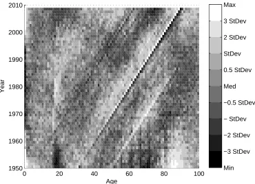
Visual inspection of the heat map of residuals in Figure 5 shows us that a) there appear to be additional age/period effects in the data, most obvi-ously centred on age 0 and age 18 and b) there is a clear need for a cohort

0 20 40 60 80 100 −0.04

−0.03 −0.02 −0.01 0 0.01 0.02

Age

β_x f(x)

(a) Age functions

1950 1960 1970 1980 1990 2000 2010 −20

−15 −10 −5 0 5 10 15 20

Year Corr = 0.94

Non−Parametric Parametric

(b) Period functions

Figure 3: Age and period functions for Stage 2 of the general procedure

0 20 40 60 80 100 −0.03

−0.02 −0.01 0 0.01 0.02 0.03

Age

β_x f(x)

(a) Age functions

1950 1960 1970 1980 1990 2000 2010 −30

−20 −10 0 10 20 30 40 50

Year Corr = 1.00

Non−Parametric Parametric

(b) Period functions

Figure 4: Age and period functions for Stage 3 of the general procedure

effect in the model as shown by the prominent diagonal lines on the heat map indicating features which follow individual years of birth as they age. The evidence gleaned from the heat map plot is useful when deciding on subsequent terms, especially when trying to determine if the shape shown by an exploratory βxκt function is trying to approximate for a cohort effect

-something we believe is essential to avoid.

0 20 40 60 80 100

1950 1960 1970 1980 1990 2000 2010

Age

Year

Min −3 StDev −2 StDev − StDev −0.5 StDev Med 0.5 StDev StDev 2 StDev 3 StDev Max

Figure 5: Heat map of residuals from Stage 3

4.5

Stage 4 onwards - Additional age/period terms

The format of the GP from Stage 4 onwards follows the same pattern as for Stages 1, 2 and 3: choose an appropriate functional form for the age term in order to capture the main effect revealed by the non-parametricβxκtterm.

We have already dipped into our toolkit of age functions, most notably by using the two-parameter Gaussian function at Stage 3. Stage 4 and onwards require us to have a far greater range of functions available in the toolkit that we can potentially use. Appendix A contains a list of the parametric functions considered in this analysis.

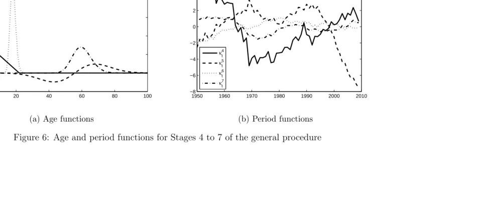
Figure 6 shows plots of the final fitted age functions f(i)(x) and trends κ(i)_t for i= 4,5,6,7. It is useful to note that the order of discovery of these functional forms provides a natural order of importance for the age terms.

The age functions we have fitted are:

• Stage 4: a broken linear function similar to the payoff of a put option, which we can associate with childhood mortality rates;9

• Stage 5: a Rayleigh function, which we associate with the postpone-ment of deaths from late middle age to old age that results from medical improvements over the past 60 years;

• Stage 6: a log-normal function centred on ages 18-19 which we associate with the peak age of the accident hump; and

• Stage 7: a normal function centred on ages 55 to 65 which may be associated with the major causes of death in late middle age, such as lung cancer and coronary heart disease and the efforts made to tackle them.

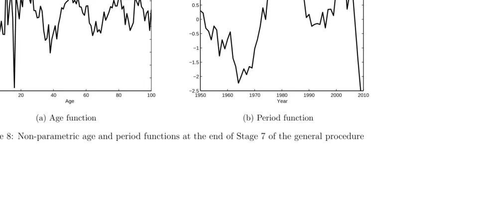
The residual heat map for Stage 7 (Figure 7) is dominated by the di-agonal lines representing the cohort effects which have been excluded from the model so far. This might lead us to conclude that we have extracted all of the important age/period effects from the data. This is confirmed by adding a further exploratory non-parametric term to the model. Whilst the resulting BIC for the model does increase, there is little structure to the βx fitted (shown in Figure 8a) except for the periodic pattern at high ages

9

This function can be thought of as a very simple linear spline with a single knot, similar to those used as basis functions in Aro and Pennanen (2011). More complex splines could also be considered as part of the toolkit of age functions.

0 20 40 60 80 100 −0.05

0 0.05 0.1 0.15 0.2 0.25 0.3

f4(x) f5(x) f6(x) f7(x)

(a) Age functions

1950 1960 1970 1980 1990 2000 2010 −8

−6 −4 −2 0 2 4 6 8

κ4 t

κ5 t

κ6 t

κ7 t

(b) Period functions

Figure 6: Age and period functions for Stages 4 to 7 of the general procedure

which is clearly trying to capture a series of cohort effects.10 _{We therefore}

conclude that, for UK male data over the sample period, there are seven distinct age/period effects in the data.

0 20 40 60 80 100

1950 1960 1970 1980 1990 2000 2010

Age

Year

Min −3 StDev −2 StDev − StDev −0.5 StDev Med 0.5 StDev StDev 2 StDev 3 StDev Max

Figure 7: Heat map of residuals from Stage 7

10

We have tested whether the use of an indicator function at age 18 or a narrow, triangu-lar “spike” function centred on this age would improve the goodness of fit. However, when using the BIC which penalises for excessive parametrisation, the use of these functions did not improve the fit of the model. The use of an indicator function also leads to mortality rates at age 18 being fit perfectly which does not accord with our desire for parsimony and may lead to discontinuous mortality rates which are not biologically reasonable.

0 20 40 60 80 100 −0.06

−0.05 −0.04 −0.03 −0.02 −0.01 0 0.01 0.02 0.03 0.04

Age

(a) Age function

1950 1960 1970 1980 1990 2000 2010 −2.5

−2 −1.5 −1 −0.5 0 0.5 1 1.5 2

Year

(b) Period function

Figure 8: Non-parametric age and period functions at the end of Stage 7 of the general procedure

4.6

Stage 8 - Cohort term

The final stage is to add the cohort parameters γt−x to yield the final model

ln(µx,t) = αx+ 7

X

i=1

f(i)(x)κ(i)_t +γt−x

Due to the limited number of observations on very early and late cohorts, we do not estimate cohort parameters in the first and last ten years of birth. Instead, we linearly interpolate these to zero for smoothness. The final model gives the cohort parameters shown in Figure 9. Adding a cohort term to the model also creates additional issues with the identifiability of the parameters, which are solved by applying extra identifiability constraints.11 _{The full set}

of identifiability constraints required by the final model produced by the GP is given in Appendix A.

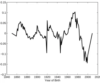
From this, we can identify the major features of interest and can try to relate them to the life histories of the affected cohorts. Most obviously, there is a clear discontinuity between years of birth 1918 and 1919. This may relate to the impact of the influenza epidemic that year. Alternatively, it could be a data artefact caused by a flood of births after the First World War distorting the assumptions used to construct exposures to risk (for a discussion, see Richards (2008)). Following this is the decline in cohort mortality observed in Willets (1999, 2004) and discussed in Murphy (2009) relating to the “golden cohort” of individuals born in the late 1920’s and early 1930’s. We also observe a further (although smaller) discontinuity between 1945 and 1946 relating to the end of the Second World War, strengthening the data artefact argument presented in Richards (2008). We are unsure what demographic significance the excess cohort mortality observed for years of birth between 1960 and 1980 has. These are individuals currently aged between 30 and 50 and therefore we have limited mortality experience data for them and so any attempt at assigning demographic significance is somewhat speculative. However, this feature is robust when adjusting the range of the data for the model and when additional age/period terms are added. This feature will be significant for projecting mortality rates if this excess mortality is continued later into life. Finally, we observe a distinct cohort effect for individuals born around the year 1900 (which again is robust to the model and data

11

This issue is discussed in Hunt and Blake (2015c).

1840 1860 1880 1900 1920 1940 1960 1980 2000 2020 −0.2

−0.15 −0.1 −0.05 0 0.05 0.1 0.15

Year of Birth

Figure 9: γt−x cohort effects from Stage 8 of the general procedure

specification). This may be due to the formative impact of experience during the First World War as young men and the lifetime health effects this may have induced.

5

Testing the final model

Our final model consists of the seven age period terms described in Table 1 plus terms for the static life table αx and the cohort parameters γt−x.

Figure 10 shows (on a logarithmic plot) the contribution each of these terms makes to improving the goodness of fit (measured by the BIC) of the model. It can be seen that the majority of the improvement in goodness of fit comes from the first three age/period terms. However, the other terms (as well as being statistically and demographically significant) are still important

Term Description f(i)(x)∝ Demographic Significance 1 Constant 1 General level

of mortality 2 Linear x−x¯ “Gompertz slope”,

rectangularisation 3 Normal exp−(x−x)ˆ2

σ2

Young adult mortality 4 “Put option” (xc −x)+ Childhood

mortality 5 Rayleigh (x−xˆ) exp (−ρ2(x−xˆ)2_{) Postponement of}

old age mortality 6 Log-normal 1

xexp

−(ln(x)−ˆx)2

σ2

Peak of accident hump 7 Normal exp−(x−x)ˆ2

σ2

Late middle / old age mortality

Table 1: Age/period terms in the final model

in describing genuine structure in the data such as the level of inequality in lifespan in the population, described by measures such as the entropy or Gini coefficient of the life table (for instance, see Shkolnikov et al. (2003)). Without them, the cohort term as the final catchall term added to the model -would attempt to capture this structure, leading to it being wrongly specified and generating inaccurate and implausible forecasts of mortality rates when projected.

Our final model should, ideally, satisfy the desirable properties relating to the adequacy and goodness of fit of the model discussed in Section 2. Specifically

1. it should provide a good and parsimonious fit to the data (which should have been achieved through the model fitting procedure);

2. it should extract all of the significant structure from the data, leaving residuals which are independent and identically distributed; and

Static 1 2 3 4 5 6 7 8 Final 104

105 106

Stage

BIC

×

−1

Figure 10: Improvement in goodness of fit at different stages of the general procedure

3. it should give parameter estimates which are robust to small changes in the data.

To test for structure within the standardised deviance residuals, we ex-tend the procedures in Dowd et al. (2010b). We first plot the heat map shown in Figure 11. This shows an apparent lack of any major age/period or cohort features and there are very few “hot” and “cold” regions or clusters in the plot. We then calculate the sample moments of the residuals which are shown in Table 2. With large exposures and death counts and assum-ing the residuals have constant variance, we can use an approximation to assume that they are N(0,1) variables under the null hypothesis and so use the Jarque-Bera statistic to test for this.

The critical statistic for the Jarque-Bera test at 95% is 5.99, whilst at 99%

0 20 40 60 80 100 1950

1960 1970 1980 1990 2000 2010

Age

Year

Min −3 StDev −2 StDev − StDev −0.5 StDev Med 0.5 StDev StDev 2 StDev 3 StDev Max

Figure 11: Heat map of residuals from Stage 8

it is 9.21. This means that we decisively reject the assumption of normality for the standardised deviance residuals. Next, we consider the correlations of the residuals with those adjacent in the age and period directions, i.e.

ρX_x =corr(ǫx−1,., ǫx,.)

ρT_t =corr(ǫ.,t−1, ǫ.,t)

Figure 12 shows the plot of these correlations against age and year and the relevant statistics if we test against the null hypothesis of independence (a two-tailed test at 95% significance) for the final model from the general procedure. Clearly, the hypothesis of independence is not supported overall. Testing these jointly (i.e., as a series of independent binomial trials where the probability of failure is 5% under the null) confirms the lack of independence in both the age and period directions at the 99% level.

Residual Standard Residual Residual Jarque-Bera mean deviation skewness kurtosis statistic General procedure -0.01 0.94 -0.03 3.38 37.70

Lee-Carter -0.02 0.98 0.47 9.75 11,700 PCA 0.00 0.94 0.06 3.26 21.25

Table 2: Properties of the residuals from Stage 8 of the general procedure and the Lee-Carter and PCA models

This lack of normality and independence should be investigated further. In practice, this may be due to isolated outliers (often caused by data errors) or due to structural changes within the data. This would cause the variance of the residuals to change with age or time. Plots of the residuals from the model against age, period and cohort (not shown) indicate that there are no extreme outliers that would need to be investigated and that the variance of the residuals is roughly constant. Therefore, it is probable that there is un-explained structure remaining within the data which is not captured by the model. However, comparing these results to those from the PCA model and other models such as the Lee-Carter model show that the GP gives results which are at least as good as those from alternative mortality models.12

We also perform a number of tests of the robustness of the model to changes in the data. These include:

1. Fitting the model to different periods of data by increasing the start date sequentially from 1950 to 1980;

2. Bootstrapping the standard deviance residuals using a method based on the procedure of Koissi et al. (2006) to test the extent of parameter uncertainty; and

3. Removing ages and years from the data by setting their weights to zero to test that none of the age/period functions are overly sensitive to specific ages and years.

The first of these tests is based on the procedure in Cairns et al. (2009). Graphs of the fitted parameters (not shown but available from the authors)

12

We will compare the relative performance of alternative mortality models in Section 6.

1960 1980 2000 −1

−0.5 0 0.5 1

Year

Correlation

0 50 100

−1 −0.5 0 0.5 1

Age

Correlation

1960 1980 2000

−5 0 5

Year

Test Statistic

0 50 100

−5 0 5

Age

Test Statistic

Figure 12: Correlations and tests statistics for residuals from the general procedure

indicate that the model fits similar patterns for the evolution of the different κ(i)_t period functions and slowly varying age functions as the age range of the data is changed.

The second robustness test we perform is to look at parameter uncertainty under residual bootstrapping. Standard bootstrapping techniques, such as that implemented by Koissi et al. (2006) were developed for use with the Lee-Carter model and assume that the residuals from the model are indepen-dent. However, this assumption is not valid.13 _{Nevertheless, for simplicity,}

13

More recently, stratified (see D’Amato et al. (2011)) and block-bootstrapping (see Liu and Braun (2010)) procedures have been used, as have those based on geo-statistical techniques which look at the correlation structure across residuals (see Deb´on et al. (2008, 2010)).

we implement an approach based on this method of residual bootstrapping in order to test our final model for parameter uncertainty. This method sam-ples randomly from the fitted residuals and adds them to the fitted mortality surface to generate artificial death counts, to which the model is refitted to generate new parameter estimates. In this fashion, the degree of parameter uncertainty can be ascertained. The plots in Figure 13 depict fan charts (see Dowd et al. (2010a)) showing the 90% confidence interval for the pe-riod and cohort parameters produced by this bootstrapping procedure using 1,000 simulations. As can be seen, the underlying pattern of the parameters remains unchanged and there is no evidence to suggest that any terms are not significant when allowance is made for parameter uncertainty. The age functions are not shown, but these are considerably more robust to the effect of parameter uncertainty than the period and cohort effects.

As a final test of the model, we systematically remove ages and years from the data by setting their weights to zeros and then refitting the parameters. This tests if any of the fitted functions are overly sensitive to the specific rows or columns of the data grid, and the model’s ability to interpolate sensibly for missing data. Figures 14 and 15 shows the impact of this analysis on the cohort parameters γt−x and on the age/period terms f

(6)_{(x) and κ}(6) t .14

As can be observed, while removing specific ages and years can distort the cohort parameters at the end of the range of data, it does not substantially affect those estimated across more data points in the centre of the range. κ(6)_t is also robust under this analysis.15_{. We are therefore satisfied that our final}

model is robust under small changes to the data.

14

This age/period term was chosen as the most specific age function fitted and therefore probably the most susceptible to uncertainty under this analysis.

15

Corresponding graphs for the age functions and other period functions, not shown here, also show considerable robustness.

1950 1960 1970 1980 1990 2000 −60 −50 −40 −30 −20 −10 0 10 20 30 40

(a) κ(1)_t

1950 1960 1970 1980 1990 2000 −25 −20 −15 −10 −5 0 5 10 15 20 25

(b)κ(2)_t

1950 1960 1970 1980 1990 2000 −15 −10 −5 0 5 10 15 20

(c) κ(3)_t

1950 1960 1970 1980 1990 2000 −5

0 5 10

(d) κ(4)_t

1950 1960 1970 1980 1990 2000 −8 −6 −4 −2 0 2 4

(e)κ(5)_t

1950 1960 1970 1980 1990 2000 −2.5 −2 −1.5 −1 −0.5 0 0.5 1 1.5

(f)κ(6)_t

1950 1960 1970 1980 1990 2000 −8 −6 −4 −2 0 2 4 6

(g)κ(7)_t

1850 1900 1950 2000 −0.25 −0.2 −0.15 −0.1 −0.05 0 0.05 0.1 0.15

(h) γt−x

Figure 13: Parameter uncertainty due to residual bootstrapping

1950 1960 1970 1980 1990 2000 2010 −2.5

−2 −1.5 −1 −0.5 0 0.5 1 1.5

Year

(a) κ(6)_t

0 20 40 60 80 100

0 0.05 0.1 0.15 0.2 0.25 0.3 0.35

Age

(b) f(6)(x)

1840 1860 1880 1900 1920 1940 1960 1980 2000 2020 −0.2

−0.15 −0.1 −0.05 0 0.05 0.1 0.15

Year of Birth

(c)γt−x

Figure 14: Parameter uncertainty due to removal of one age of data

1950 1960 1970 1980 1990 2000 2010 −2

−1.5 −1 −0.5 0 0.5 1 1.5

Year

(a) κ(6)_t

0 20 40 60 80 100

0 0.05 0.1 0.15 0.2 0.25 0.3 0.35

Age

(b) f(6)(x)

1840 1860 1880 1900 1920 1940 1960 1980 2000 2020 −0.2

−0.15 −0.1 −0.05 0 0.05 0.1 0.15

Year of Birth

(c)γt−x

Figure 15: Parameter uncertainty due to removal of one year of data

6

Comparison with alternative models

The model produced by the GP in Section 5 had some unexplained structure according to our analysis of the residuals. How serious a problem is this? Perhaps the best way to answer this question is to compare the model from the GP with some alternative mortality models: the LC model (as the most widely used mortality model) and a method based on principal component analysis which extends the Lee-Carter approach with multiple age/period and cohort terms.

The LC model, introduced in Lee and Carter (1992) has subsequently been much studied, developed and extended, most notably in the work of Lee (2000), Brouhns et al. (2002), Booth et al. (2002), Renshaw and Haberman (2003), Renshaw and Haberman (2006) and Hyndman and Ullah (2007). It has rapidly become the benchmark mortality model against which others are compared (for instance in Cairns et al. (2009) or Plat (2009)) and so is a natural starting point for comparing the model produced by the GP against. However, it is a relatively simple model with only one age/period term and no cohort term, and so we would expect the GP to give significantly better fits to the data.

The singular value decomposition used to fit the model to data in Lee and Carter (1992) is a particular implementation of principal component analysis (PCA) - see Huang et al. (2009) for more details. It is therefore the natural exten-sion of the Lee-Carter methodology capable of giving multiple age/period terms. It finds age and period functions that explain the maximum amount of variance (across the period dimension) in the model. PCA has long been used in the study of mortality rates: for example Wilmoth (1990) used it to detect higher order age/period functions, Booth et al. (2002) and Renshaw and Haberman (2003) both proposed its use to extend the

Lee-Carter model with additional age/period terms and the models of Hyndman and Ullah (2007) and Yang et al. (2010) used it directly to fit multiple age/period

ef-fects. However, it cannot directly find cohort efef-fects. Therefore a direct comparison of PCA with our model is not appropriate.

In order to compare procedures, we use a method similar to that used in Wilmoth (1990). We first use PCA to find age/period functions for ln(µx,t)

in the absence of cohort effects. We then add a cohort effect to the

lying model and use the PCA age/period effects as the starting point when maximising the Poisson log-likelihood using the algorithms in Appendix A. This process is repeated for different numbers of age/period terms and the model with the highest BIC selected for comparison against our final model.

6.1

Results

Table 3 compares the three models and shows the goodness of fit to our dataset. The LC is a single factor model and so it is unsurprising that the other two models give considerably better fits to the data, although at the cost of a far greater number of parameters. The PCA method also requires substantially fewer age/period terms to achieve a very similar goodness of fit to the model produced by the GP. Because each of these age functions has approximately one hundred free parameters compared with a maximum of two using the GP, this does not result in a more parsimonious model, however. Further, as we are primarily interested in the evolution of mortality rates over the period, we consider that it is desirable to have a high proportion of the parameters relating to the period and cohort effects of interest. This is not the case in the PCA model.

Model No. A/P No. free Log- BIC terms parameters likelihood

General procedure 7 679 −3.09×104 _−3.38×104

Lee-Carter 1 259 −5.13×104 _−5.25×104

PCA 3 735 −3.07×104 _−3.39×104

Table 3: Goodness of fit for the different models

Figures 16 and 17 show the age and period functions for the GP and PCA procedure - the age and period functions for the LC model are the same as the non-parametric terms shown in Figure 2. We find it difficult to assign demographic significance to the age functions in the LC and PCA models. The cohort parameters for the GP and PCA models are shown in Figure 18 - there is no corresponding plot for the LC model due to the absence of a cohort term. Here it is worth noting the similarities as well as the differences in the fitted parameters. Both approaches detect the discontinuities after the

First and Second World Wars and the increase in cohort mortality for years of birth around 1900 and between 1960 and 1980.

However, there are substantial differences in both the magnitude and the pattern of cohort parameters. Cohort effects for the GP are less pronounced than those from the PCA procedure. In addition, the PCA model fails to find a sustained decrease in cohort mortality for the “golden cohort” discussed previously. Most seriously, there appear to be large cohort effects at the beginning and end of the range of years of birth which are not explainable demographically. We believe that these effects are trying to compensate for the second and third age functions in the PCA model, which do not tend to zero at high ages (as shown in Figure 17a). This has very serious effects when these models are projected into the future. We therefore believe that the cohort parameters produced by the GP are more biologically reasonable and demographically significant than those fitted by the PCA procedure.

Table 2 above shows the moments and results of the Jarque-Bera tests on the residuals for the three approaches. We note that none of the three models tested give normally distributed standardised residuals, although the residuals from the GP and PCA models come considerably closer than those from the LC model.

We also compare plots of the residual heat maps in Figure 19 and test for correlation amongst the standardised deviance residuals in Figure 20 from the Lee-Carter and PCA models in Figure 20 - comparable plots for the GP are shown in Figures 11 and 12 respectively. The heat maps for the Lee-Carter and PCA models shows obvious clusters in the fitted residuals, indicating that there is still substantial structure remaining in the residuals of the PCA model. The LC residuals in particular show the clear need for a cohort term to capture the impact of the cohorts born after the First and Second World Wars. The PCA model yields residuals which are closer to normality than the GP, although they still do not pass the Jarque-Bera test. The correlations across residuals from the PCA procedure are higher than from the GP. Probably this is due to the smaller number of age/period terms. However, adding additional terms to the PCA model results in worse BICs and therefore will not improve the goodness of fit. This reinforces the conclusion that there is still structure in the data which is not adequately captured by the PCA model.

0 20 40 60 80 100 −0.05

0 0.05 0.1 0.15 0.2 0.25 0.3

Age

f1(x) (GP) f2(x) (GP) f3(x) (GP) f4(x) (GP) f5(x) (GP) f6(x) (GP) f7(x) (GP)

(a) Age functions

1950 1960 1970 1980 1990 2000 2010 −60

−50 −40 −30 −20 −10 0 10 20 30 40

Year κ1

t (GP)

κ2 t (GP)

κ3 t (GP)

κ4 t (GP)

κ5 t (GP)

κ6 t (GP)

κ7 t (GP)

(b) Period functions

Figure 16: Age and period functions for the general procedure

0 20 40 60 80 100 −0.04

−0.03 −0.02 −0.01 0 0.01 0.02 0.03

Age β1

x (PCA)

β2 x (PCA)

β3 x (PCA)

(a) Age functions

1950 1960 1970 1980 1990 2000 2010 −60

−40 −20 0 20 40 60

Year

κ1 t (PCA)

κ2 t (PCA)

κ3 t (PCA)

(b) Period functions

Figure 17: Age and period functions for the PCA model

1840 1860 1880 1900 1920 1940 1960 1980 2000 2020 −0.3

−0.2 −0.1 0 0.1 0.2 0.3 0.4 0.5 0.6

Year of Birth

GP PCA

Figure 18: Cohort parameters for the GP and PCA models

0 20 40 60 80 100 1950

1960 1970 1980 1990 2000 2010

Age

Year

Min −3 StDev −2 StDev − StDev −0.5 StDev Med 0.5 StDev StDev 2 StDev 3 StDev Max

(a) Lee-Carter

0 20 40 60 80 100

1950 1960 1970 1980 1990 2000 2010

Age

Year

Min −3 StDev −2 StDev − StDev −0.5 StDev Med 0.5 StDev StDev 2 StDev 3 StDev Max

(b) PCA

Figure 19: Residual heat maps for the Lee-Carter and PCA models

1960 1980 2000 −1 −0.5 0 0.5 1 Year Correlation

0 50 100

−1 −0.5 0 0.5 1 Age Correlation

1960 1980 2000 −20 −10 0 10 20 Year Test Statistic

0 50 100

−20 −10 0 10 20 Age Test Statistic (a) Lee-Carter

1960 1980 2000 −1 −0.5 0 0.5 1 Year Correlation

0 50 100

−1 −0.5 0 0.5 1 Age Correlation

1960 1980 2000 −5

0 5

Year

Test Statistic

0 50 100

−5 0 5 Age Test Statistic (b) PCA

Figure 20: Residual correlations across age and period for the Lee-Carter and PCA models

7

Conclusions

As the level of interest in longevity risk increases, it becomes increasingly im-portant to be able to construct more sophisticated mortality models reliably and robustly. These will need to capture most of the identifiable structure in mortality rates within the data - which calls for more terms - but to do so with the smallest number of free parameters - which calls for parsimony. Where cohort effects are believed to be real and important, they will need to be captured by the model. However, they must also be clearly distinguished from age/period effects in order that they can be projected correctly. This, in practice, means that all the significant age/period effects must be identi-fied before any attempt is made to estimate the cohort effect. Finally, terms within the model should be capable of being associated with underlying bio-logical or social processes. This requires judgement to be used to guide their projection and aid their communication with other, non-technical, stakehold-ers who are subject to longevity risk and wish to undstakehold-erstand the implications.

In this paper, we have introduced a new, general procedure for construct-ing mortality models. The general procedure is driven by forensically exam-ining the data to provide evidence for the selection of each and every term in the final model produced. We believe this improves the goodness of fit of the model parsimoniously and with demographic significance. We have applied the general procedure to a specific dataset, associated each term generated with an underlying demographic and/or socio-economic factor for the population being modelled, analysed the residuals to confirm that there is no identifiable structure remaining in the data which is not captured by the model, and compared the results with those from other methods of con-structing mortality models.

The general procedure requires the modeller to engage intelligently with the data and make various subjective decisions in its implementation. It is not a “black box” algorithm which can be deployed mechanically on various datasets, but rather requires a substantial investment of time to understand the underlying forces driving mortality within the population of interest and how these forces can be represented mathematically. But far from this being a disadvantage, we would argue that our approach accords perfectly with good model building practice, which seeks to move beyond a purely algorith-mic approach in order to understand better the underlying structure of the

data.

In conclusion, we believe that the general procedure is capable of produc-ing models which are in accordance with the desirability criteria of adequacy of fit to the data, demographic significance, parsimony, robustness and com-pleteness (by including sufficient terms to cover all ages and cohorts).

However, we are aware that in order to be practically useful, a good fit to historical data needs to be accompanied by the ability to use the model to make reliable forecasts of future mortality rates. Projecting models with multiple age/period and cohort terms consistently is a difficult problem as the historical time series are often highly correlated and display curvature, outliers or subtle trend changes which need to be accommodated (as have been described in Li and Chan (2005); Li et al. (2011) and Coelho and Nunes (2011)). We therefore intend to address this issue in Hunt and Blake (2015a) and Hunt and Blake (2015d).

A

Appendix: Algorithms and toolkit of

func-tion

In order to implement the general procedure, we need the ability to introduce new terms to existing models and to fit these to data. At each stage, all pa-rameters within the model are freely estimated (although the values found at previous stages are used as convenient starting points for later stages of the maximisation algorithm). The exception to this is when new non-parametric terms are added to the model and the previously fitted age functions are not re-estimated as this often leads to model instability. As these terms are added purely for exploratory purposes and all parameters will be re-estimated once they are replaced with suitable parametric forms, we do not believe this will have a significant impact on the final model.

As we have central exposures to risk from the Human Mortality Database (Human Mortality Database (2014)), we adopt a Poisson likelihood maximi-sation approach which enables us to do this quickly and efficiently. This procedure is based on that implemented in Brouhns et al. (2002) and is de-scribed in Algorithm 1 at high level below.

Algorithm 1 Algorithm for Poisson likelihood maximisation

1: Set initial starting values and calculate initial log-likelihood

2: while Increase in log-likelihood less than threshold value (e.g. 10−2)do

3: Maximise log-likelihood with respect toαxholding all other parameters

constant

4: for Each age/period term i do

5: Maximise log-likelihood with respect toκ(i)_t holding all other param-eters constant

6: Maximise log-likelihood with respect to free-parameters θ(i) in age function f(i)_(x;θ(i)_{) or with respect to β}

x holding all other

parame-ters constant

7: end for

8: Maximise log-likelihood with respect to γt−x holding all other

param-eters constant if model contains a cohort term

9: Impose identifiability constraints through use of invariant transforma-tions

10: Calculate updated log-likelihood

11: end while

12: Calculate residuals and BIC

The fitting algorithm used by the general procedure differs from the Brouhns et al. (2002) method in that the log-likelihood is maximised with respect to each set of parameters sequentially rather than simultaneously. It could be argued that this may lead the algorithm to find local rather than global maxima for the parameter values. In practice, we have not found this to be an issue and believe it can be largely resolved through finding the full set of identification issues for the parameters within the model (as discussed in Hunt and Blake (2015b,c)). The maximisation of each set of parameters (i.e. ξ =αx, βx, κ

(i)

t , γc, θ(i)) is done as per Algorithm 2 below.

This is nothing more than the repeated application of the Newton-Raphson procedure. The parameter φ ∈ (0,1] is a simple scaling which can be low-ered to improve the stability of parameter estimates (albeit at the cost of increasing the run time of the algorithm). In most cases, the parameter sets are treated as vectors meaning that ∂2_L

∂ξ2 is the Hessian matrix. However, this

matrix usually has a diagonal structure (e.g. ∂2_L

∂αx∂αy = 0 for x 6= y) which

Algorithm 2 Algorithm for maximisation of individual parameters

1: Start with values for maximisation passed from parent algorithm

2: while Increase in log-likelihood less than threshold value (e.g. 10−4)do

3: Calculate first derivative of log-likelihood with respect to parameters

∂L ∂ξ

4: Calculate second derivative of log-likelihood with respect to parameters

∂2_L ∂ξ2

5: Update estimate of parameters ˆξ =ξ−φ

∂L ∂ξ ∂2L ∂ξ2

6: Impose simple identifiability constraints, e.g. on the level ofκ(i)_t , using invariant transformations

7: Update fitted surface µx,t and log-likelihood 8: end while

9: Return updated parameter estimates, fitted mortality rates and

log-likelihood to parent algorithm

simplifies the implementation significantly.

Models produced by the GP will not be fully identified and so will require additional identifiability constraints to be robustly estimated. A discussion of the origin and nature of this lack of identifiability and the selection of ap-propriate identifiability constraints was given in Hunt and Blake (2015b) and Hunt and Blake (2015c). In summary, we impose the following identifiability constraints upon the final model from Stage 8.

X

t

κ(i)_t = 0 ∀i (7)

X

x

|f(i)(x;θ(i))|= 1 ∀i (8)

X

y

nyγy = 0 (9)

X

y

nyγy(y−y¯) = 0 (10)

X

y

nyγy((y−y¯)2−σy) = 0 (11)

Not all of these constraints will be applicable at all stages (e.g., the

straints in Equations 9, 10 and 11 will not apply to models without a cohort term) whilst for models with a non-parametric age function, we require the additional constraints below.

X

x

|βx|= 1 (12)

X

x

βxf(i)(x;θ(i)) = 0 ∀i (13)

(14)

We refer to Equations 8 and 12as the normalisation of the age function. In contrast to some authors (e.g. Haberman and Renshaw (2009)) we do not re-quire that age functions are non-negative. In order to normalise age functions with free parametersθ(i), we must modify the form of the age function so that

P

x|f(i)(x;θ(i))| is not a function ofθ(i). This means that the normalisation

scheme in Equation 8 holds as θ(i) _{is varied when fitting the model. This is}

usually achieved by multiplying it by a “self-normalisation” functionN(θ(i)). This was discussed in greater depth in Hunt and Blake (2015b). Equation 13 is only applied in exploratory models with a non-parametric term in order to maximise the distinctness of the age/period terms.

The functions in the toolkit we have developed so far are given in Table 4 along with the free parameters they require and the self-normalisation func-tions N(θ(i)). In this, the age range is assumed to run from age 1 to age X with ¯x= _X1 PX

x=1x andσx = 1 X

PX

x=1(x−x¯)2. Some of these normalisations

are only approximate or are true up to a constant, so it is still necessary to rescale the age functions after applying Algorithm 2 to optimise the value of the free parameters. Similar definitions for ¯y and σy are used in Equations

9, 10 and 11.

References

Aro, H., Pennanen, T., 2011. A user-friendly approach to stochastic mortality modelling. European Actuarial Journal 1 (S2), 151–167.

Booth, H., Maindonald, J., Smith, L., 2002. Applying Lee-Carter under con-ditions of variable mortality decline. Population Studies 56 (3), 325–36.

Figure 21: Age functions in toolkit

0 20 40 60 80 100 −0.02 −0.01 0 0.01 0.02 0.03 0.04 0.05 0.06 0.07 Age Constant Linear Quadratic "Put" "Call"

0 20 40 60 80 100 −0.05 0 0.05 0.1 0.15 0.2 0.25 0.3 Age Exponential Gumbel Normal Log−Normal Ellipse Rayleigh

Brouhns, N., Denuit, M. M., Vermunt, J., 2002. A Poisson log-bilinear re-gression approach to the construction of projected lifetables. Insurance: Mathematics and Economics 31 (3), 373–393.

Cairns, A. J., Blake, D., Dowd, K., 2006a. A two-factor model for stochastic mortality with parameter uncertainty: Theory and calibration. Journal of Risk and Insurance 73 (4), 687–718.

Cairns, A. J., Blake, D., Dowd, K., 2006b. Pricing death: Frameworks for the valuation and securitization of mortality risk. ASTIN Bulletin 36 (1), 79–120.

Cairns, A. J., Blake, D., Dowd, K., Coughlan, G. D., Epstein, D., Ong, A., Balevich, I., 2009. A quantitative comparison of stochastic mortality models using data from England and Wales and the United States. North American Actuarial Journal 13 (1), 1–35.

Campos, J., Ericsson, N. R., Hendry, D. F., 2005. General-to-specific mod-eling: An overview and selected bibliography. Federal Reserve Discussion Papers.

Coelho, E., Nunes, L. C., 2011. Forecasting mortality in the event of a struc-tural change. Journal of the Royal Statistical Society: Series A (Statistics in Society) 174 (3), 713–736.