Advancing integrability for strings in AdS3/CFT2

City, University of London Institutional Repository

Citation

: Lloyd, Thomas (2016). Advancing integrability for strings in AdS3/CFT2.

This is the accepted version of the paper.

This version of the publication may differ from the final published

version.

Permanent repository link:

Link to published version

:

Copyright and reuse:

City Research Online aims to make research

outputs of City, University of London available to a wider audience.

Copyright and Moral Rights remain with the author(s) and/or copyright

holders. URLs from City Research Online may be freely distributed and

linked to.

Advancing Integrability for

Strings in AdS

₃

/CFT

₂

Thomas Lloyd

A thesis submitted for the degree of

Doctor of Philosophy

City University London

Department of Mathematics

Contents

1 Introduction: gauge/gravity dualities 13

1.1 Elements of String Theory . . . 13

1.2 The Maldacena Conjecture . . . 15

1.2.1 The planar limit . . . 17

1.3 AdS3/CF T2 dualities . . . 18

1.3.1 AdS3 backgrounds from brane constructions . . . 18

1.3.2 DualCF T2 . . . 20

2 Strings and Integrability 23 2.1 Strings in Anti-de Sitter Space . . . 23

2.1.1 The String Sigma Model and its symmetries . . . 23

2.1.2 Gauge-fixing . . . 25

2.1.3 Strings on plane-waves . . . 27

2.2 Integrability of classical strings . . . 29

2.2.1 Classical Integrability . . . 30

2.2.2 Classical strings . . . 31

2.2.3 Coset model on R×S2 and a single-cut algebraic curve 34 2.3 Outline of following chapters . . . 37

3 Finite-gap equations and massless modes 39 3.1 The Penrose Limit of AdS3×S3×S3×S1 and the spectrum of bosonic strings on plane-waves . . . 39

3.2 Quasimomenta and finite-gap equations . . . 43

3.2.1 Finite-gap equations . . . 43

3.2.2 The Generalised Residue Conditions . . . 45

3.3 Strings on R×S1×S1 ⊂AdS3×S3×S3 . . . 47

3.3.1 Coset representatives and quasimomenta . . . 48

3.3.2 Solutions in lightcone gauge . . . 51

3.3.3 Solutions in static gauge . . . 54

3.4 Finite-gap equations with Generalised Residue Conditions . . . 58

3.5 Chapter conclusions and outlook . . . 61

4 Quantum corrections to the algebraic curve 63 4.1 Fluctuations around zero-cut classical solutions inAdS3×S3×T4 64 4.1.1 Examples . . . 72

4.2 Fluctuations around zero-cut classical solutions inAdS3×S3× S3×S1 . . . 74

4.2.1 Examples . . . 78

5 The worldsheet S-matrix of AdS3×S3×T4 with mixed-flux 83

5.1 Supergravity background and Killing spinors . . . 85

5.2 Bosonic action in lightcone gauge . . . 88

5.3 The Green-Schwarz Action . . . 90

5.3.1 Fixing kappa gauge . . . 94

5.4 Supercurrents . . . 96

5.5 The algebra A and its representations . . . 99

5.5.1 Near-plane-wave algebra . . . 99

5.5.2 Exact representations . . . 105

5.6 The all-loop S-matrix . . . 109

5.6.1 su(1|1)2-invariant S-matrices . . . 110

5.6.2 psu(1|1)4-invariant S-matrices . . . 112

5.7 Chapter conclusions and outlook . . . 114

6 Conclusion 117

A Index conventions 121

B Gamma matrices 123

C Quasimomenta residues for general solutions on R×S3×S1 125

D Generalised residue condition for AdS5×S5 129

E Generalised residue condition for AdS4×CP3 131

F Generalised residue condition for D(2,1;α)2 in mixed grading133

G Decoupled S1 mode 135

H Spinor identity 137

I Spin-connections 139

J Quartic Supercurrents 143

K Poisson brackets 147

L S-matrix elements 149

List of Figures

1 Particle worldline and string worldsheets . . . 13

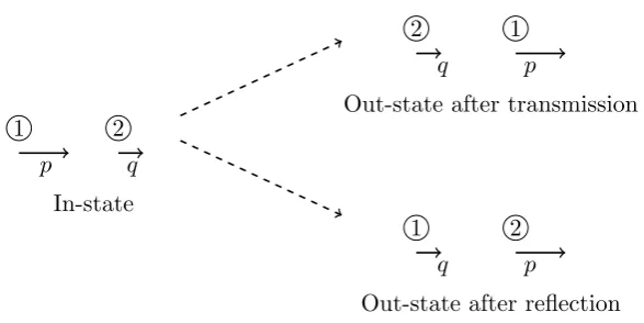
2 String interactions . . . 14

3 Planar and non-planar Feynman diagrams . . . 18

4 D1-D5 and D1-D5-D5’ systems . . . 20

5 Analytic structure of example 1-cut quasimomentum . . . 37

6 P SU(1,1|2) modes . . . 67

Acknowledgements

I would like first and foremost to thank my supervisor Bogdan Stefa´nski for

all the guidance, advice and support he has given me over the last three and a half years. I have greatly enjoyed working with him and being his student. It

was a pleasure to collaborate with Olof Ohlsson Sax, Alessandro Sfondrini and

Bogdan, and I am very grateful to them and to Riccardo Borsato for the many useful discussions I have had with them on numerous topics of the work that

went into this thesis. I would also like to thank Nikolay Gromov, Alessandro

Torrielli, Arkady Tseytlin and Kostya Zarembo for helpful discussions and comments on this work at earlier stages.

During my doctoral studies I have been financially supported by an STFC

studentship.

Finally I would like to thank my family and my partner Jenny for the

countless ways, both small and large, they have supported me throughout this

Declaration

The work contained in this thesis was carried out by the author while studying

for the degree of Doctor of Philosophy at City University London. Parts of this work were previously published in the co-authored papers [1] and [2].

Powers of discretion are granted to the University Librarian to allow this thesis to be copied in whole or in part without further reference to the author.

This permission covers only single copies made for study purposes, subject to

Abstract

In this thesis we develop techniques of integrability in the study of dualities

between two-dimensional conformal field theories and theories of closed strings on three-dimensional Anti-de Sitter background geometries. For several years

after integrability was first applied to the 3d/2d dualities, it was an unanswered

question how to incorporate the so-called “massless modes” of these theories into the integrability machinery. Here we tackle this problem in several

con-texts. We show that in the classical integrable description of closed strings

the implementation of the string Virasoro constraints needs to be modified for geometries with multiple factors where massless modes are present. We

show further that with the correct implementation of the Virasoro constraints,

massless modes can be included in integrability techniques for obtaining quan-tum corrections to physical quantities such as the energies of string solutions.

Lastly, we consider the scattering of fundamental string excitations and derive

Chapter 1

Introduction: gauge/gravity

dualities

1.1

Elements of String Theory

String theory is a unified theory of quantum gauge and gravity interactions.

The concept of a fundamental relativistic string can be understood by com-parison with a point-particle. A single particle propagating in a spacetime

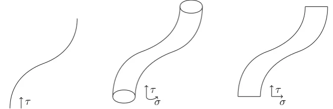
with coordinates Xm can be described by its worldlineXm(τ) giving its posi-tion at each moment in proper timeτ. A fundamental string extends along a spacelike coordinateσ in addition to a timelike coordinateτ, and is described by its worldsheet Xm(τ, σ). The coordinate σ may be identified periodically in which case we call the string closed, otherwise it is an open string.

τ

τ σ

τ σ

Figure 1: The worldline for a particle (left) and worldsheets for a closed string (centre) and open string (right).

There are two parameters that describe fundamental strings. One is the dimensionless string coupling constant gs, which controls the strength of the

string splitting and joining interactions. In perturbative calculations an

ex-pansion ings corresponds to a sum over different string topologies. The other

fundamental parameter is the string scalels, or equivalently the string tension T, which are related by

T = 1 2πα0 =

1 2πl2

s

, (1.1)

where the parameter α0 is called the Regge slope. The string can be excited along vibrational modes, and the tension determines the energy of these

ex-citations. The low energy limit is α0 → 0. The natural way to study string theory perturbatively is to consider a dual expansion in the parametersα0and

gs. If one first expands ings then each term in this expansion corresponds to

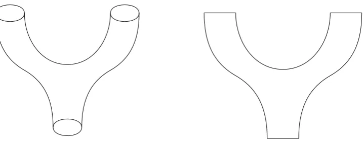
Figure 2: String interactions: splitting of a closed string (left) and an open string (right).

topology, there is an expansion in α0.

String theory places demands on the spacetime in which it is constructed in

order to maintain physical consistency. In particular, superconformal

invari-ance requires that the spacetime be ten-dimensional and obey the supergravity generalised Einstein equations [3]. The simplest possible background is

ten-dimensional Minkowski spacetime. In the Green-Schwarz formalism [4] for

implementing supersymmetry, the theory is described by the evolution of a string not just in spacetime, but in superspace. This means that in addition

to the bosonic fieldsXm(τ, σ) there are spacetime fermionic fieldsθI(τ, σ). In the theory of type IIB superstrings that we will focus on, there are two such fermions, I = 1,2, and each is a Majorana-Weyl spinor of the same chirality. This means that each has 16 independent real components and in total there

are 32 supersymmetries.

In the spectrum of vibrational excitations of the closed superstring in the

critical dimension, the lowest energy states are massless. The bosonic states

transform as a spacetime tensor which can be decomposed into symmetric traceless, antisymmetric and trace parts. The first of these is a graviton field

Gmn, the secondBmn is referred to as the B-field and the last Φ is called the

dilaton. The B-field acts as a potential for a Neveu-Schwarz-Neveu-Schwarz (NS-NS) 3-form Hmnp. There are also Ramond-Ramond (R-R) fields arising

from odd and even rank potentials in the type IIA and type IIB theories

respectively. For the backgrounds of interest to us in this thesis the only non-zero R-R field is the R-R 3-formFmnp. Consistency of the theory implies

conditions on these fields which are identical to the equations of motion arising

from a particular ten-dimensional action. This action is that of type IIB supergravity [5–8]. Since in the low energy limit α0 → 0 other states above these massless states are suppressed, we conclude that type IIB supergravity is the low energy limit of type IIB superstring theory.

Open strings have endpoints, and so variation of the string action places

boundary conditions at these endpoints in addition to equations of motion.

CHAPTER 1. INTRODUCTION: GAUGE/GRAVITY DUALITIES

where we set ∂σXm= 0 at the endpoints, and Dirichlet boundary conditions,

where we fix Xm _{to be constant at the endpoints. If we choose Neumann}

boundary conditions for endpoints in spatial dimensionsm= 0. . . p, then the string endpoints are fixed along the remaining (10−p−1) dimensions, i.e. they are constrained to lie in a (p+ 1)-dimensional hypersurface, which we call a Dp-brane [9, 10].

D-branes have a dual identity in string theory. As well as their role as endpoints for open strings, they also appear as particular solutions called p -branes in supergravity, meaning that they are dynamical objects of superstring

theory in their own right [11]. As objects in string theory they couple to R-R fields. For type IIB supergravity, stable Dp-branes exist forpodd. In addition there are 5-branes that are also charged under the bosonic B-field, the so-called

NS5-branes.

The low energy spectrum of open type II strings again starts with massless

states. Consider the excitations of an open string ending on a Dp-brane from the point of view of the (p+ 1)-dimensional space in which the brane prop-agates. From this perspective the bosonic massless excitations of the open

string divide into those perpendicular to the brane, which appear as massless

scalars, and those parallel to the brane, which appear as a gauge vector. In this way the excitations on a single Dp-brane describe a U(1) gauge theory. This gauge symmetry can be enhanced to a non-abelian one if we consider open strings on not just a single Dpbrane, butN branes coincident with one another. In this case we can introduce labels called Chan-Patton factors [12]

which specify which of the N branes the endpoints of an open string are on. Counting these labels for both ends of the string, each state now comes with

a multiplicity ofN2. In particular the gauge group is enhanced toU(N) [13]. The explicit form of the resulting gauge theory is that of a Yang-Mills the-ory [14].

1.2

The Maldacena Conjecture

The Maldacena conjecture [15] relates strings on a background involving a factor of (d+ 1)-dimensional Anti-de Sitter (AdS) space to a conformal field theory (CFT) inddimensions. The canonical example of this conjecture states that the theory of type IIB strings propagating on a background ofAdS5×S5

with constant R-R 5-form flux is dual to the gauge theory known as N = 4 Super-Yang-Mills [16, 17]. This conjecture arises by considering first type IIB

strings in flat space with a stack of N coincident D3-branes which will then backreact on the geometry. The system is examined in the low energy limit

from two perspectives corresponding to the two guises of D-branes as endpoints

The supergravity metric arising from the stack of D3-branes is [18]

ds2 = p1

f(r) −dt

2₊ 3

X

i=1 dx2_i

!

+pf(r) dr2+r2dΩ2₅

, (1.2)

wheredΩ2

n is the usual round metric inn-dimensions, andr is the associated

radial coordinate. The functionf(r) is given by

f(r) = 1 +R

4

r4 , (1.3)

so that this solution has a horizon atr= 0. Finally the parameterRis related to the string parametersgs and α0 and the number N by

R4= 4πgsα02N . (1.4)

The numberN of D3-branes in the construction enters the low energy super-gravity solution in the 5-form R-R fluxF5, with

Z

S5

F5=N . (1.5)

The Maldacena conjecture arises by looking at the low energy limit of this setup of D3-branes from two perspectives. In the first, we have a set of open

strings propagating on the branes and closed strings in the bulk (the rest of

spacetime away from the branes). In the low energy limit, the interaction between closed and open strings is subleading and so we have two decoupled

systems. The dynamics of the open strings are described by a gauge theory

on the four-dimensional space spanned by the D3-branes, with gauge group

SU(N). This gauge theory is N = 4 Super-Yang-Mills (SYM). It has been shown that its beta function is exactly zero [19–22], and so it is a CFT.

In the second perspective, we replace the open strings by the backreaction

of the D3-branes on the geometry, that is we have a system of closed strings

propagating in the spacetime (1.2). One part of the low energy limit of this spacetime is again free supergravity coming from low energy excitations of

strings in the bulk away from the branes. Another comes from the

near-horizon geometry. The energy E of an excitation at distance r from the horizon is related to the energy E∞ that an observer at infinity sees by the

redshift factor

E∞=f(r)−

1

4E . (1.6)

Low energy excitations in the bulk are unable to be brought close to the

horizon. Therefore, in the low energy limit of the second perspective we again have two decoupled systems, one of which is free supergravity. The other

CHAPTER 1. INTRODUCTION: GAUGE/GRAVITY DUALITIES

Anti-DeSitter space in the form

ds2_AdSn =−dt2+ 1

r2dr 2₊

n−2

X

i=1

dx2_i . (1.7)

By comparing the two perspectives, we are led to infer that this is an equivalent

system toN = 4 SYM.

In the SYM gauge theory describing the dynamics of the open strings,

the physical parameters are the Yang-Mills coupling gY M and the number of

colour charges N. The duality relates these to the string parameters gs and α0 via the following identifications:

gs= g_{Y M}2

4π , R4 α02 =g

2

Y MN . (1.8)

The supergravity description of the backreaction is appropriate when the

radius of curvature R of the spacetime is much larger than the string scale,

Rls. On the CFT side of the duality this is the regiong2Y MN 1. Hence

the duality relates low energy strings to the strongly coupled sector of the

gauge theory, and vice versa. This is an example of a strong-weak duality.

It means that perturbative string quantization and perturbative field theory expansions cannot be compared, making the duality harder to test. On the

other hand, it promises the possibility of solving problems of strong coupling

by solving in the dual weakly coupled regime.

1.2.1 The planar limit

The “large N” or ”planar” limit of the field theory corresponds to taking

gY M →0,N → ∞ but keeping the ’t Hooft couplingλdefined as λ≡g_{Y M}2 N = R

4

α02 (1.9)

fixed. It has been known for a long time [23] that in this limit of

Yang-Mills theories there is a simplification of perturbative calculations. The only

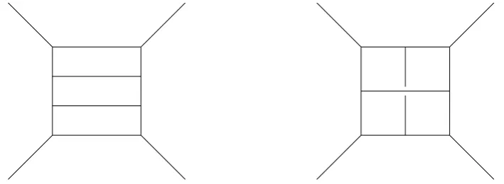
contributions that survive the limit come from Feynman diagrams that are planar, meaning they can be drawn in two dimensions without crossing, see

figure 3. We can see from equation (1.8) relating the parameters that on the string side this limit corresponds to gs →0, i.e. to a limit of free strings with

no interactions. Therefore, the planar limit of the Maldacena conjecture is a

duality between planar N = 4 SYM and free superstrings onAdS5×S5. It is in the planar limit that integrability appears. On the gauge side,

integrability appears in terms of an integrable spin-chain [24]. We will discuss

Figure 3: A planar (left) and non-planar (right) Feynman diagram.

1.3

AdS

/CF T

dualities

1.3.1 AdS3 backgrounds from brane constructions

Alongside the AdS5/CF T4 correspondence outlined above, another duality

was posited [15] which related strings on a background containing AdS3 to a two-dimensional CFT. The brane construction leading to this duality was a system ofN1 D1-branes together withN5D5-branes.1 Four spatial dimensions

along which the D5-branes extend are compactified on a T4. The D1-branes then extend along the same remaining non-compact spatial dimensions which

theD5-branes span. The metric for this setup is

ds2 = √1

f1f5

(−dt2+dx2₁) +pf1f5 dr2+r2dΩ23

+

s

f1 f5

9

X

i=6

dx2_i (1.10)

where

f1(r) = 1 +

gsα0N1

vr2 , f5(r) = 1 +

gsα0N5

r2 , v= V_T4

(2π)4_α02 , (1.11)

andVT4 is the volume of theT4. The low energy limit involvingα0 →0 is taken

together with theT4compactification in such a way thatvremains finite. Just as in the D3-brane setup, there is a horizon at r = 0 and in the low energy limit the near-horizon geometry decouples from that of the bulk. In this case

the near-horizon limit r→ 0 produces the background AdS3×S3×T4. The

radii of both AdS3 and S3 are equal and given by

R= gsα

0√_N

1N5

√

v . (1.12)

In both the D3-brane stack and the D1-D5 system, the branes couple to

R-R fields, and a full description of the supergravity solution includes these fields. In the case of the D1-D5 system, there is a 3-form R-R flux F(3) which in the near-horizon limit is a constant, proportional to the volume forms on AdS3

1_{This D1-D5 system was already well-studied for its use in describing black-hole}

CHAPTER 1. INTRODUCTION: GAUGE/GRAVITY DUALITIES

and S3. More generally, superstrings on this background can be supported by a mix of R-R and NS-NS fluxes. Supergravity backgrounds supported

by these mixed fluxes are generated by NS5-branes and fundamental strings

in addition to D1-branes and D5-branes. There is a one-parameter family of supersymmetric backgrounds involving this mix of branes, and so a

one-parameter family of dualities with mixed fluxes. Namely, when we set the

AdS3 radius to 1, the fluxes can be written as

F = ˜q(Vol(AdS3) + Vol(S3)) , H =q(Vol(AdS3) + Vol(S3) (1.13)

where

q2+ ˜q2 = 1 . (1.14)

Another set of AdS3/CF T2 dualities is found involving the background AdS3×S3×S3×S1. The radiiR+ and R− of the two three-spheres in this

background are related to the radius R ofAdS3 as follows:

1

R2 =

1

R2 +

+ 1

R2

−

, (1.15)

which is required to make the background a consistent supergravity solution. We introduce a parameter α defined by

1

R2₊ = α R2 ,

1

R2₋ =

1−α

R2 , (1.16)

and again we have a one-parameter family of such backgrounds. This

parame-terαappears in the symmetry superalgebra of these backgrounds as discussed in section 1.3.2. When giving worldsheet expressions on this background in this thesis we will generally use the alternative parameter φdefined by

α = sin2φ . (1.17)

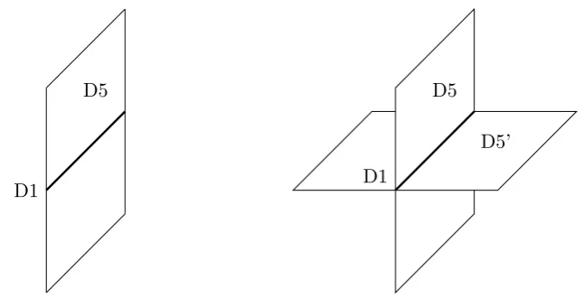
The brane construction used to construct this background [26–28] is that of a D1-D5-D5’ system, which can be thought of as a D1-D5 system to which

is added a second set of D5-branes, compactified on the directions transverse

to the first set and vice versa. We denote this setup in the following diagram:

1 2 3 4 5 6 7 8 9

D1 ×

D5 × × × × ×

D50 × × × ×

where×’s mark spatial directions spanned by the various branes, see also fig-ure 4. One subtlety is that this construction actually leads to the geometry of

D5

D1

D5

D5’

D1

Figure 4: Three-dimensional representation of a D5 system (left) and D1-D5-D5’ system (right).

from RtoS1.

Early progress in studying strings on theseAdS3backgrounds was achieved

using worldsheet CFT techniques [29–36] to study the pure NS-NS

back-grounds, which are related to the pure R-R backgrounds by S-duality. The use of integrability in AdS/CF T dualities, which we discuss in the following chapter, avoids the need for applying an S-duality and also makes it possible

to study the mixed-flux backgrounds.

1.3.2 Dual CF T2

Identifying the dual conformal gauge theory to the AdS3 string background

is a harder problem than in the case ofAdS5/CF T4. In particular, the gauge

theory describing the open string dynamics in the low energy limit is not con-formally invariant. The dual CFT is instead conjectured to arise from the

renormalization group flow to the IR of this gauge theory. Another important

difference between thisAdS3/CF T2duality and the canonicalAdS5/CF T4 du-ality is the presence of a large moduli space [37]. N = 4 SYM is a theory with only two tuneable parameters: λ and N. However, there are various scalars which arise from the open string dynamics on the D1-D5 system which have non-zero expectation values. The field content of the D1-D5 systems contains

vector multiplets and hypermultiplets. Both of these multiplets contain scalar

fields. The two branches of the moduli space are the Higgs branch, where the hypermultiplet scalars have non-zero vacuum expectation values, and the

Coulomb branch where the vector multiplet scalars have non-zero vacuum

expectation values. The IR Higgs branch CFT is conjectured to be dual to

AdS3 strings [15], because it is this branch that corresponds to motion of

the D1-branes inside the D5-branes and so is consistent with the near-horizon

picture.

The CFT can also be understood by treating the D1-branes as an instanton

CHAPTER 1. INTRODUCTION: GAUGE/GRAVITY DUALITIES

in the moduli space where this instanton shrinks to zero size that the spin-chain picture which integrability relies on emerges. It has been believed for

some time that this moduli space can be obtained as a deformation of the

spaceSymN(T4), the symmetric space ofN copies ofT4, where N =N1N5 is the product of the numberN1 of D1-branes and N5 of D5-branes [40]. Early

work on the CFT side of the AdS3 dualities was undertaken by studying the SymN(T4) orbifold theories and their deformations in [41–44].

In identifying the CFT dual ofAdS3×S3×S3×S1, there is the additional

problem that in studying the open string dynamics on the brane construction,

one has to deal with the difference between the factor ofRin the near-horizon

limit and the factor of S1 in the final geometry. Partly owing to this, the dual conformal theory to this background has proved among the most

elu-sive in all AdS/CF T dualities, with early work studying it in [45] and since then in [46, 47]. One thing that is known is the necessary superconformal

symmetry algebra of the dual CFT. All the brane constructions discussed in

this section preserve 16 real supersymmetries. In two dimensions these can be decomposed by chirality and we say that we have N = (4,4) supersym-metry in two dimensions. Unlike for example N = 4 supersymmetry in four dimensions, we can distinguish further between different supersymmetry al-gebras [48]. The CFT dual to AdS3×S3×T4 preserves what is called the

small N = (4,4) algebra, while the CFT dual to AdS3×S3 ×S3×S1 pre-serves the large N = (4,4) algebra. These algebras are infinite-dimensional. Their finite-dimensional subgroups which can be defined globally are the

alge-bras of the groups of superisometries of the dual string backgrounds, namely

P SU(1,1|2)2 _forAdS

3×S3×T4 andD(2,1;α)2 forAdS3×S3×S3×S1. The

parameterα here is the same one appearing in the geometry that defines the relative radii of the two three-spheres as in equation (1.16).

In this thesis we will focus on studying the string side of the AdS3/CF T2

dualities introduced in this chapter. In the next chapter we introduce the

Chapter 2

Strings and Integrability

In this chapter we will outline the basics of the ideas and techniques used in

this thesis. Full definitions of the ideas we introduce here will generally be

given in the main text.

2.1

Strings in Anti-de Sitter Space

2.1.1 The String Sigma Model and its symmetries

Our starting point is the standard bosonic string action on a curved back-ground, the non-linear sigma model. For a background with spacetime metric

Gmn(X) and supported by a non-zero two-form gauge fieldBmn(X), the action

is

Sbos=−

1 4πα0

Z

d2σ√−γγαβGmn(X) +αβBmn(X)

∂αXm∂βXn , (2.1)

whereXm are the spacetime coordinates,γαβ is the worldsheet metric,

carry-ing indices associated to the worldsheet coordinatesσα = (τ, σ) andαβ is the alternating tensor. Since we will be interested in critical superstrings of type

IIB, the background spacetime will always be ten-dimensional. In particular

we will be interested in theAdSbackgrounds discussed in the previous chapter and in limits of these backgrounds.

As in flat space, this action possesses several symmetries at the classical

level, namely invariance under reparametrisation of the worldsheet

coordi-nates,

σα→fα(σ) (2.2)

and Weyl or scale invariance under transformation of the worldsheet metric

γαβ →Ω2(σ)γαβ . (2.3)

As well as the equations of motion coming from varying the action with

respect to the spacetime fieldsXm, the action (2.1.1) also gives us the Virasoro constraints [49],

Gmn(X)

˙

Xm±X0m X˙n±X0n= 0 (2.4) arising, as in flat space, from variations with respect to the worldsheet metric.

The full superstring action is given by the bosonic action above together

latter is given by a Green-Schwarz action [4, 50], but this now requires us to describe spinors on a curved background. We give the details of how this

Green-Schwarz action is described in chapter 5 and an alternative formulation

of the fermionic action in a group theoretic description in section 2.2.2. For now we will note several important points about the Green-Schwarz action.

For type IIB strings the fermionic fields are two 10-dimensional spinors

θI,I = 1,2. These are Majorana-Weyl spinors, meaning they satisfy first the

reality condition that they are equal to their Majorana conjugate,

θ_IC =θI , (2.5)

and second that they have definite chirality,1

Γ0123456789θI=θI . (2.6)

In appendix B we give an explicit basis of ten-dimensional gamma matrices

Γ which we use throughout this thesis whenever one is needed, and define

Majorana conjugation in terms of this explicit basis. Each of the two con-ditions above reduces the number of independent components of the spinors

by half, so having started with 32 complex components they end up with 16

independent real components.

As discussed in chapter 1, the backgrounds of interest to us arise in the near-horizon limit of particular brane constructions, and as such the resulting

backgrounds are supported by the p-forms which are the charges of these branes. In particular, the AdS3 backgrounds of interest to us can in general be supported by a combination of R-R and NS-NS 3-form fluxes. The fermionic

fields θI couple to themselves and to the bosonic fields through these 3-form fluxes, just as the bosonic fields Xm couple amongst themselves through the NS-NS B-field in the bosonic action (2.1.1).

In flat space, the fermionic kappa symmetry which we discuss below can be fixed in such a way that the Green-Schwarz action becomes quadratic in

fermionic fields. For a generic curved background this is no longer possible.

However, the general type II action is known to quartic order in fermions [51] and for the backgrounds of interest here, kappa symmetry can be fixed in such

a way that there are no higher order terms above this [52]. Regardless, for our purposes in this thesis it will suffice to use the action to quadratic order

in fermions.

The full Green-Schwarz action is manifestly invariant under spacetime

su-persymmetry, which is a global fermionic symmetry. There is also another

fermionic off-shell symmetry of the theory, called kappa-symmetry, which is a gauge symmetry. Fixing a particular gauge for this symmetry is

neces-1_{Since we are interested in type IIB strings, both spinorsθ}

1andθ2have the same chirality,

CHAPTER 2. STRINGS AND INTEGRABILITY

sary to show explicitly that the Green-Schwarz action is also invariant under worldsheet supersymmetry. We will introduce it here by the simplest theory

in which such a symmetry shows up [53]: the worldline action of a massless

superparticle given by

S = Z

dτ1 e

˙

Xm−iθ¯Γmθ˙

2

. (2.7)

This action is invariant under the transformation

δθ=iΓmpmκ , δXm =iθ¯Γmδθ , δe= 4eθκ ,˙¯ (2.8)

where pm is the conjugate momentum to Xm and κ = κ(τ) is any spinor

function of proper time.

Gauge-fixing this symmetry has the effect of reducing the number of

in-dependent fermionic components by half. This last fact can be observed as

follows. The equation of motion for θis (Γmpm) ˙θ= 0. Meanwhile the

analo-gous statement of the Virasoro constraints for the superparticle action is the

vanishing of the total momentum

p2 = 0 , pm = ˙Xm−iθ¯Γmθ .˙ (2.9) which in turn implies (Γmpm)2 = 0. Hence the rank of the matrix Γmpm is

at most half of its size (as follows for example from the rank-nullity theo-rem). Indeed as there are no other constraints on the momentum, it is exactly

half. We conclude that half of the components of θ do not actually enter the equations of motion and cannot be physical. This ensures that the number of independent real components of the fermions is equal to the number of

transverse bosons, as is required for consistent worldsheet supersymmetry.

This argument we have presented to show how kappa symmetry arises for a superparticle in flat space in fact extends to the full superstring action in flat

space [4] and further to any supergravity background [54]. Kappa symmetry

is as such a symmetry of the full string action.

2.1.2 Gauge-fixing

In this section we discuss the various gauge choices that can be made to fix

the symmetries discussed in the previous section. In looking at these gauge

choices we draw attention to the issues that arise on curved backgrounds in general, and on the AdS spaces of interest to us in particular.

One gauge choice that can be made is to use reparametrisation of the

worldsheet coordinates and Weyl invariance to fix conformal gauge, where the worldsheet metric is fixed to be everywhere equal to the 2d Minkowski metric,

is no longer true for generic curved backgrounds as we discuss further below.

Lightcone gauge [55] is given by choosing lightcone spacetime coordinates

x± =ψ±t , (2.10)

then fixing

x+=p+τ (2.11)

and then using the Virasoro constraints to solve forx− in terms of the remain-ing fields. On curved backgrounds, as in flat space, it is a convenient gauge to quantize the theory in because the Virasoro constraints are solved at the

clas-sical level before quantizing. For supersymmetric theories, the use of lightcone

gauge is complicated by the need to combine it with a choice of kappa gauge, and the resulting choice for the latter is often referred to as lightcone kappa

gauge.

As mentioned above, lightcone gauge cannot be consistently taken with

conformal gauge for a generic background spacetime. The question of when these gauges are consistent was addressed in [56, 57], where it was found that

these gauges can be simultaneously imposed for spacetimes which possess a

covariantly constant null Killing vector, in addition to satisfying the usual conditions for Weyl invariance such as being in the critical dimension. The

origin of this additional requirement is that if (2.11) can be imposed, then the vector

V = ∂

∂_x−

(2.12)

is such a constant null Killing vector. Note that theAdSspacetimes of interest to us do not satisfy this condition2, and as such the fixing of lightcone gauge for these backgrounds [58, 59] does not use the conformal gauge. We will discuss in section 2.1.3 examples of non-flat spacetimes where this condition

is satisfied.

Static gauge consists of the choice

t=κτ (2.13)

where t represents the usual time coordinate of AdS. In some sense, it rep-resents a half-way choice between lightcone quantization and conformal

quan-tization, since the number of degrees of freedom is reduced by one below the critical dimension, but is still one higher than the number of physical degrees

of freedom. However, at the classical level it is often a natural choice to study

particular string solutions where the Virasoro constraints can be checked ex-plicitly. These solutions can then be studied semiclassically in the static gauge

by requiring the timelike bosonic field to not receive quantum corrections.

Be-2

Although they possess null Killing vectors, they are not covariantly constant ones. This is necessary so that, for example,G−−= 0, and thus the Virasoro conditions have a linear

CHAPTER 2. STRINGS AND INTEGRABILITY

cause of its frequent use in classical and semiclassical string solutions, it is generally encoded into the classical description of strings in the integrability

framework which we discuss below.

Different kappa gauges have been studied. One of these is known as the coset gauge [60], which for example on AdS3×S3×T4 is [61]

Γ6789θI = 0 , (2.14)

where 6789 are the T4 directions. In this gauge the Green-Schwarz super-string action reduces to a coset action. Any such action as this admits an

algebraic structure and is classically integrable [62]. However, the coset kappa

gauge does not lead to a conventional quadratic kinetic term for the massless fermions, but rather a kinetic term which is higher order in fields. Such a

higher order kinetic term is not convenient for the introduction of canonical Poisson brackets. As such we will find it convenient, following [63–65], to use

a different kappa gauge,

Γ+ηI= 0 , Γ+χI = 0 , (2.15)

where ηI and χI are suitable redefined fermions. We will discuss the exact

field redefinitions required in chapter 5. Here we will simply mention that η,

χ are defined so as to make them neutral under the U(1)’s associated with shifts in tand ψ.

2.1.3 Strings on plane-waves

We turn now to strings on backgrounds which are not Anti-de Sitter, but a

class of spacetimes known as plane-wave spacetimes. These arise in particular

limiting process from other geometries. Studying strings on these backgrounds is an interesting question in its own right because they provide a rare example

where it is understood how to exactly quantize the theory even in the presence of curvature. We will be interested in them because of the guide they provide

to understanding strings on AdS spaces. Once we fix a particular lightcone gauge, if we consider an expansion in transverse fields, the leading order terms are the same as those in the plane-wave theory, and higher order terms can

be treated as corrections away from the plane-wave. In particular, considering

string theory on the plane-wave limit of the backgrounds of interest to us will provide us with what we can think of as a set of elementary excitations of the

theory with a set of associated masses.

The general metric for a plane-wave spacetime is

ds2=−4dx+dx−+

D−2

X

i=1

mix2i(dx+)2+ D−2

X

i=1

where mi is in general allowed to be a function of x+. For our purposes as

will shortly become clear we will be interested solely in considering mi to be

constants, and of course we are also considering only the critical dimension

D = 10. Plane-wave metrics of the form (2.16) are defined within the larger class of pp-wave spacetimes as those which possess a covariantly constant

null Killing vector, and hence as explained in section 2.1.2, strings on these

backgrounds can be quantized similarly to strings on flat space. When this is done, the bosonic sigma model action reduces to that of 8 free bosons whose

masses are given by the constants mi [66, 67]. This can be compared with the

action of free massless bosons which arises from string theory on flat space, which is of course exactly what the metric (2.16) reduces to when all mi = 0.

It was observed in [66, 68] that one particular plane-wave background rep-resents another maximally supersymmetric solution of type IIB string theory

possessing 32 supercharges, alongside flat space and AdS5×S5. This case is

when each of the massesmi is the same,mi =m, and the bosonic background

is supplemented by a 5-form R-R flux given by

F+1234 =F+5678= 2m . (2.17)

This background is obtained by taking a Penrose limit of theAdS5×S5 back-ground [69, 70]. A Penrose limit involves selecting a particular null geodesic in

spacetime and considering a limit in the near-vicinity of the geodesic such that the resulting metric remains non-singular. In the case of the possible Penrose

limits ofAdS5×S5, the choice of null geodesic which preserves maximally

su-persymmetry in the IIB theory is a null geodesic whose spacelike part simply moves around the equator of the sphere.

The theory of IIB superstrings on the plane-wave background obtained by a Penrose limit of AdS5×S5 can be quantized in the lightcone gauge. The

question of how this Penrose limit relates to the duality with N = 4 SYM was first considered in [70]. As well as a geometric limit of the background spacetime, the plane-wave IIB theory can also be thought of as a limit where

particular Noether charges are taken to be large. In particular, given the

energy E and an angular momentum J associated to motion around the S5

equator, we are considering a limit where

E → ∞ , J → ∞ (2.18)

This “large charge” limit can be carried over naturally to the gauge side of the duality, where we will be taking the dimensions of the relevant operators to be

large. The limit is called the BMN limit (Berenstein, Maldecena, Nastau) [70]

in the context of AdS/CFT, and perturbative calculations have been made on both sides of the duality in this limit.

Pen-CHAPTER 2. STRINGS AND INTEGRABILITY

rose limit which maximises supersymmetry, and consequently leading to a theory which is most likely to be solvable. For the case of AdS3×S3 [71–75]

the appropriate limit is one where again the spacelike component of the null

geodesic in the limit runs around the equator of the sphere, so the geodesic is given by

t=ψ=τ . (2.19)

ForAdS3×S3×S3 [76, 77] we choose a null geodesic which runs around both

equators of the spheres. In this case there is an additional parameter involved

in choosing the limit according to which linear combination one choose the geodesic to take over the two spheres. The choice which turns out to maximise

supersymmetry is [46, 76]

t=τ , ψ1 = cos2φ τ , ψ2 = sin2φ τ . (2.20)

For these particular Penrose limits, the number of supersymmetries of the

two theories are not just preserved, but are in fact enhanced, to 20

supersym-metries in the case of theAdS3×S3×S3 theory [76] and 24 in the case of the

AdS3×S3 theory. [78] After these limits, the metrics of the two backgrounds

are given by equation (2.16) with masses

{mi}={1,0} (AdS3×S3×T4)

{mi}={1,cosφ,sinφ,0} (AdS3×S3×S3×S1) (2.21)

where each mass comes with a multiplicity of four bosons and four fermions

in the former case, and two in the latter.

As can be seen, both backgrounds have massless fundamental excitations in their plane-wave limit. This is a new feature of theAdS3backgrounds which

does not show up in higher dimensions. At the level of the Penrose limit of the

geometry, the factors of T4 and S1 are essentially decoupled in the limiting procedure and so remain flat subspaces in the plane-wave spacetime. These

flat subspaces give rise to four and one massless boson(s) respectively. The

S1 background has another massless boson coming from a transverse direction around both S3 _{equators. Each of the massless bosons has a superpartner}

massless fermion. Despite their simple origin from the Penrose limit

perspec-tive, the massless modes have proven difficult to implement in the integrability descriptions of the full theories, as we will discuss further, and developments

on how to incorporate them will constitute a major recurring aspect of the

work in this thesis.

2.2

Integrability of classical strings

We now turn to the subject of integrability. We will begin by introducing the

integrability as defined for finite-dimensional systems can be extended to field theories with infinitely many degrees of freedom, using the so-called Lax

for-mulation. Then we will discuss how these ideas apply to classical strings, and

discuss how, for particular backgrounds, the string sigma model can be cast in an integrable form.

2.2.1 Classical Integrability

The original notion of integrability is that of a Liouville integrable classical system. This concept applies to finite-dimensional dynamical systems, usually

Hamiltonian systems with 2n degrees of freedom given by positions qi and

momenta pi depending on a time parameterτ, with evolution in τ governed

by a Hamiltonian H. In particular, for any function f(qi, pi), its evolution in

time is given by

˙

f ={f, H}. (2.22)

where the Poisson bracket of two functionsf, g,{f, g}is defined to be

{f, g}=X

i

∂f ∂qi

∂g ∂pi

− ∂f

∂pi ∂g ∂qi

. (2.23)

The system is defined to be Liouville integrable if there arenfunctionsfi that

are in involution,

{fi, fj}= 0 , (2.24)

one of which is the Hamiltonian, and hence all are conserved. For such

sys-tems, the Arnold-Liouville theorem guarantees that there exists a coordinate system in which all momenta are constant, and the dynamical evolution of the

positions is uniform motion around a torus.

The key idea in this original notion of integrability is that there be as many

conserved quantities as degrees of freedom in the theory. For the extension to

field theories with infinitely many degrees of freedom, it is natural to assume integrability must mean there are infinitely many conserved quantities, but it

is unclear whether this should be a sufficient condition by itself. One way to

proceed is to use the ideas of the Lax formalism [79], which can be defined for finite-dimensional integrable systems and which then generalise naturally

to field theories. This works as follows: suppose square matrices Land M of sizencan be built out of the variables of the theory such that the dynamical equations of the theory can be written as

˙

L= [M, L]. (2.25)

Then it follows that

d dτtr(L

k_{) = 0 (2.26)}

CHAPTER 2. STRINGS AND INTEGRABILITY

The obvious generalisation of the Lax formalism to infinite-dimensional systems is simply to take the Lax pair (L, M) to be infinite-dimensional matri-ces. We achieve the same result however by introducing the so-called spectral

parameterzand considering a one-parameter family of matrices (L(z), M(z)). The advantage of this approach is that we can deduce properties of a particular

solution, or obtain equations that characterise different solutions, by

consid-ering the analytic structure of the matrices on z.

The generalisation of equation (2.25) to field theories relies on something which is unique to two-dimensional field theories, and hence these are the

only ones for which we can use integrability.3 When d = 2 we can regard the Lax pair as being made up of the two components of a connection on a vector bundle, (L(z), M(z))→(Lτ(z), Lσ(z)) and then the condition that this

connection Lα be flat,

∂αLβ(z)−∂βLα(z)−[Lα(z), Lβ(z)] = 0, (2.27)

is the generalisation of equation (2.25).

In the finite-dimensional case we saw the conserved charges arising from

the Lax formulation as the eigenvalues ofL. Now in the case of field theory, we expect to have an infinite set of conserved charges arising in a similar way. We

need now to define the monodromy matrix as the path-ordered exponential of

the Lax connection,

M(z, τ) = Pexp Z 2π

0

dσLσ . (2.28)

From the flatness ofLα, this obeys the evolution equation

∂τM(z, τ) = [Lτ(2π, τ, z), M(z, τ)] (2.29)

and so

∂τtr(Mk) = 0 , (2.30)

and now the eigenvalues ofM are conserved quantities. By expanding in the spectral parameter z, typically ub oiwers if 1_z around z = ∞, we obtain an infinite set of conserved charges.

2.2.2 Classical strings

In this section we will give an overview of how classical integrability shows up

in particular string backgrounds. The key idea is that for these backgrounds,

3

the classical string action can be formulated as a coset action for a supergroup whose bosonic subgroup represents the isometries of the relevant background.

An action of this form was first given for strings onAdS5×S5 in [81], following

the earlier use [82] of a coset action to describe strings on flat space. A key feature of many examples of cosets describing strings on AdS spaces is that

they admit a Z4 automorphism [83].4 This allows a flat Lax connection to be

written down for the theory [62] and hence the theory is classically integrable in the manner discussed in the previous section. Superspaces admitting a Z4

automorphism are called semisymmetric spaces [85]. Following [61, 86, 87],

we will find it convenient to describe the setup of strings on semisymmetric spaces in a general group-theoretic form, and this can then be specialised to

the particular cases of interest to us by specifying the relevant supergroups.

We consider a coset G/H consisting of a supergroup G equipped with a

Z4 automorphism Ω :G→ G, and where H ∈G is the invariant subspace of

Ω. To form a string action on such a space, the elements in G are functions over the worldsheet, g(τ, σ) ∈ G and we can relate these group elements to the usual bosonic and fermionic fields of the Green-Schwarz action in some

(non-unique) way. We form the standard Maurer-Cartan one-forms jα in the

Lie algebra g ofG,

jα=g−1∂αg , (2.31)

and then the automorphism Ω also acts on these one-form currents, giving a decomposition of the algebra which we denote

jα = 3

X

n=0

j_α(n) , (2.32)

where the automorphism Ω acts as

Ωj(_αn)=inj_α(n) . (2.33)

In this decomposition j(0) and j(2) represent the bosonic parts of the algebra and j(1) and j(3) the fermionic parts.

The string action is given by

S =

√

λ

8π

Z

d2σStr√−γγαβj_α(2)j_β(2)+αβj_α(1)j_β(3) , (2.34) where Str denotes the unique invariant bilinear form ongwhich all superspaces of interest to us possess.56 It does not depend onjα(0) which is invariant under

4_{This was first shown for the case ofAdS}

5×S5 explicitly in [84]. 5

See e.g. [88]

6_{IfGis realised as a group of supermatrices, this bilinear form is the supertrace:}

Str

A B C B

CHAPTER 2. STRINGS AND INTEGRABILITY

Ω, and as such is an action on the coset G/H. We should note that that in general the coset action (2.34) does not describe a consistent string action. It is necessary to check, given a particular group G, that the background associated to it is a consistent string theory background (for example, that it is a supergravity solution etc.).

A Lax connection for the action (2.34) is given by

Lα=jα(0)+ z2+ 1

z2₋₁j (2) α −

2z z2₋₁

1

−γγαβ βγ_j(2)

γ

+ r

z+ 1

z−1j

(1) α +

r

z−1

z+ 1j

(3)

α . (2.35)

The flatness condition for this Lax connection is equivalent to the equations of motion arising from the action (2.34), together with the Maurer-Cartan

equa-tions for the flatness of the current (2.31). The Virasoro constraints are an

additional requirement which needs to be imposed in addition to the flatness of the Lax connection. They arise, just as in the usual sigma model, from

vari-ations of the worldsheet metric. In conformal gauge they are given explicitly

by

Str

j_τ(2)2+j_σ(2)2

= Str

j_τ(2)j_σ(2)

= 0 . (2.36)

As discussed in the previous section, given a monodromy matrix M aris-ing from a flat Lax connection we know that the eigenvalues of M are time-independent, so they are functions only of the spectral parameter z. We diagonalise the monodromy matrix arising from the Lax connection (2.35) in

terms of a particular Cartan basisHl forGas

M(z) =U−1(z)epl(z)Hl_{U(z) . (2.37)}

We refer to the functionspl(z) as the quasimomenta of the system. The infinite

set of conserved charges that characterise the theory as being integrable show

up in the quasimomenta in a convenient way. We find that expanding at large

z, the behaviour of any quasimomentum pl is

p(z) =−2

zQl+. . . (2.38)

where Ql is a conserved charge of the system, in fact it is a Noether charge

associated to a global symmetry. Higher terms in the expansion give an infinite set of conserved charges.

The quasimomenta pl(z) have a more interesting analytic structure than M(z). The Lax connection is defined as az-dependent function of the currents in such a way that its only singularities inz are atz=±1, and for a solution just in the bosonic sector these are simple poles. The monodromy matrix

indeed we can use these branch cuts to characterise classical string solutions. On each branch cut, the quasimomenta are required to satisfy the monodromy

condition

Alm/p_m(z) = 2πnl , z∈Cl,i (2.39)

where Alm = Str(HlHm) is the Cartan matrix of the group, Cl,i denotes the

set of cuts on the sheet for the corresponding quasimomentum pl, and /p_l is

the continuous part of the quasimomentum on the cut.

The monodromy condition (2.39) can be recast as a set of integral

equa-tions, called the finite-gap equations. We will see in detail in the following chapter how this is done. Solutions to these equations are often called the

algebraic curve. Finite-gap equations have been written down for strings on

the AdS5×S5 background, first in subsectors [89–91] and then for the full background [92]. Following this, finite-gap equations were written down for

strings onAdS4×CP3 [93], for the pure R-RAdS3 backgrounds of interest to

us in this thesis [61], for backgrounds involving AdS2 [87] and most recently for the mixed-flux AdS3 ×S3 ×T4 background [94]. One important result

of the work in this thesis is to show how the finite-gap equations need to be

modified in the presence of massless excitations.

2.2.3 Coset model on _R×S2 _{and a single-cut algebraic curve}

We will now illustrate the ideas of coset models and classical string solutions described as algebraic curves by considering a simple example: bosonic strings

onR×S2. We will take as the coset for this modelSU(2)/U(1), so the timelike

coordinate is supplementary. We parametrise elements g ∈ G = SU(2) in terms ofC2 coordinates as

g= Z1 −Z

2 Z2 Z1

!

(2.40)

where Zi ≡ Z_i∗ and |Z1|2+|Z2|2 = 1. In terms of this parametrisation the

currents (2.32) are given by

j= Z

1_dZ1+Z2_{dZ2 Z}2_dZ1_−Z1_dZ1 Z1dZ2−Z2dZ1 Z1dZ1+Z2dZ2

!

. (2.41)

For a sigma model describing bosonic strings only, theZ4automorphism of

a semisymmetric superspace is reduced to aZ2automorphism, that isGis now

a symmetric space. We can define a particular choice of this automorphism Ω acting onsu(2) in terms of its action on the Pauli matrices. A useful choice is Ω(σ1) =−σ1 , Ω(σ2) =−σ2 , Ω(σ3) =σ3 . (2.42)

CHAPTER 2. STRINGS AND INTEGRABILITY

by its diagonal and off-diagonal parts respectively. The invariant subalgebra of

su(2) under this automorphism is clearly a U(1) subalgebra, so this is indeed giving us the coset we want.

The other simplification of the general picture when considering bosonic

strings only is that we can replace the “supertrace” in the action by the usual

trace. The action is therefore

S=

√

λ

8π

Z

d2σ√−γγαβ

tr

j_α(2)j_β(2)

−∂αt∂βt

(2.43)

We can see that this action is indeed equivalent to the usual action for bosonic strings on R×S2, and in this process see also how the action of the

coset works explicitly in this case, by changing from complex coordinates Zi

to angular coordinates on S3. If we take

Z1 = cosθeiϕ , Z2= sinθeiψ (2.44)

then we find

−1

2tr

h

j(2)i2

=dθ2+ sin2θcos2θ(dϕ−dψ)2 . (2.45) The automorphism Ω selecting only the off-diagonal parts of the current is therefore giving us theS2subsector ofS3given in these coordinates byψ+ϕ= 0.

We will now look briefly at how particular solutions to the classical

evo-lution of strings on R×S2 can be readily seen to give rise to quasimomenta

possessing branch cuts. We will consider strings in conformal gauge, and so-lutions of the form

t=κτ , ϕ=−ψ=nσ , θ=θ(τ) (2.46) in the coordinates (2.44). The equation of motion for θ can be solved with the Virasoro constraints to give a general elliptic integral solution, but we can

ignore the exact form of this solution. The resulting Lax connection for this solution has a componentLσ given by

Lσ =incos(2θ)σ3−insin(2θ) z2+ 1

z2₋₁σ1−iθ˙

2z

z2₋₁σ2 . (2.47)

Now we see that for this solution the Lax connection is independent ofσ, so the path-ordered exponential required to give us the monodromy matrix sim-plifies greatly to an ordinary matrix exponential. When we then diagonalise

by

p(z) = 2π

z2₋₁

q

n2_(z2₋₁₎2_cos2_{θ+ 4n}2_z2_sin2_{θ+ (z}2_{+ 1)}2_θ˙2 _{. (2.48)}

In this form it appears thatp(z) depends onτ throughθ, but the path-ordered exponential is to be taken at any fixed τ, so given a particular solution θ(τ) we could simply substitute its values at sayτ = 0. We know that the flatness of the Lax connection means that for any θ(τ) which obeys the equations of motion, the expression in the square root here is indeed τ-independent. In fact for this solution, once we make use of the Virasoro constraints we can

explicitly rewrite it as

p(z) = 2π

z2₋₁

p

κ2_z2_+n2_(z2₋₁₎2 _{. (2.49)}

We can see from the form of p(z) in (2.49) that it indeed has simple poles atz =±1 as we always expect, and in general has four branch points. Thus we have shown that in general solutions of the form (2.46) are described by an algebraic curve with two branch cuts. In fact these two branch cuts are related,

so that we regard this solution as having onephysical branch cut. This arises through the action of theZ4 automorphism on the quasimomenta.7 Given its

action on the currents, we can find that the action of the automorphism Ω on

the general Lax connection (2.35) is

Ω(Lα(z)) =Lα

1

z

. (2.50)

Also, given a particular Cartan basis, we can write the action of Ω on the

elements of this basis via a symmetry matrix S as

Ω(Hl) =HmSlm (2.51)

and then we have a symmetry in the quasimomenta of inversion in the spectral

parameterz,

pl

1

z

=Slmpm(z) . (2.52)

In our example above, we have a single Cartan element and S is the 1×1 identity matrix (see equation (2.42)) and so our single quasimomentum p(z) must always have an even number of branch cuts. We can classify solutions

by the number of branch cuts possessed in the physical region |z|> 1. The solution (2.49) has, for κ2 > 2n2, a single branch cut in the physical region connecting two branch points on the imaginary axis, as we show in figure 5.

7_{Here with quasimomenta for the bosonic sector only, the}

Z4automorphism in fact reduces

CHAPTER 2. STRINGS AND INTEGRABILITY

Re(z) Im(z)

1 -1

Figure 5: The analytic structure of the quasimomentum (2.49). There is a single branch cut in the physical region |z| > 1, which is reflected in the region |z|< 1 by inversion symmetry. There are also the usual simple poles atz=±1.

2.3

Outline of following chapters

A common theme throughout the work of this thesis will be developing the

understanding of how the massless modes that are seen in the plane-wave

lim-its of the AdS3 backgrounds should be incorporated into the machinery of integrability. It was demonstrated initially when the coset model describing

classical dynamics of strings on these backgrounds was written down [61] that

it did not include these massless modes. However, this did not prevent progress in understanding these theories through integrability. In particular, there was

a successful programme of applying the techniques of quantum integrability

to the massive-only sector of the theories. The all-loop Bethe ansatz for the massive sector of both theD(2,1;α) andP SU(1,1|2) theories (with pure R-R flux) was calculated by directly reverse-engineering from the finite-gap

equa-tions and associated spin-chains [61, 95]8, and also by means of first obtaining the exact S-matrices from the symmetries of the theories [97–100]. In addition,

integrability played a role in direct worldsheet calculations [101–108], where

the problem of missing massless modes as in the coset model did not arise.

Chapter 3, which is based on [1], deals directly with the issue of the

mass-less modes in the coset model. It begins with a review of the Penrose limit

of AdS3×S3×S3×S1 and the bosonic sector of the spectrum of strings on the resulting plane-wave background. In this spectrum there are two massless

bosons. One arises on the factor of S1, and its absence in the coset model is unsurprising based on the symmetries of the coset. The other, which we will sometimes refer to as the “coset” massless boson, emerges on the transverse

8_{There was also progress in understanding the massless modes in the spin-chain by}

direction along the equators of the two three-spheres, and as such is within the part of the geometry which the coset describes. The key result of chapter 3

is to show how, through a correction to the way the Virasoro constraints had

previously been implemented in the coset model, this mode can be incorpo-rated. Once this correction is made, the remaining massless boson, and all

four in the T4 background, can be incorporated through U(1) quasimomenta which interact with the coset only through the corrected Virasoro constraints. Chapter 4 applies the results of chapter 3 to the semiclassical methods

of quasimomenta fluctuations, again primarily in order to show how massless

modes can appear explicitly in calculations where they were previously absent. Fluctuations of the algebraic curve had been studied previously for a variety

of solutions in theAdS3 backgrounds [104,109–111], where the massless modes were absent and had to be put back in by hand. Progress in understanding the massless fermions in this context was made in [112], where it was shown how to

include additional modes that appeared with non-zero mass in a class of

back-ground solutions containing the BMN vacuum, with energy corrections which smoothly approached that of a massless mode in the limit to the BMN

back-ground. Chapter 4 contains work which has not been previously published. In

this chapter, we combine the prescriptions of [112] with the results of chap-ter 3 to show how the semiclassical algebraic curve can produce a complete

spectrum of energy corrections for semiclassical fluctuations around classical

string solutions, including both massless and massive mode contributions. Chapter 5 is based on work in [2] which combines the extension of

inte-grability techniques into the massless sector of the backgrounds with another extension of integrability into theAdS3×S3×T4 backgrounds with mixed

R-R and NS-NS flux. These mixed-flux backgrounds have been studied through

a generalisation of the coset model [94, 113], in particular the action (2.34) requires an additional term to incorporate the Wess-Zumino (WZ) term of

the GS action. The S-matrix of the massive sector of the mixed-flux

back-grounds was studied in [114, 115]. An important difference from the pure R-R backgrounds arises in the exact dispersion relation of fundamental excitations

which was further studied in [116]. The work of chapter 5 follows on from

a project initiated in the pure R-R background in [64, 65] which constructs the exact S-matrix using symmetry arguments but working from the

Green-Schwarz action rather than the coset action. In this way massless excitations

can be included and the resulting S-matrix consists of massive-massive scatter-ing which matches results obtained from the coset action, together with sectors

for massless-massless and massive-massless scattering. Chapter 5 of this thesis

Chapter 3

Finite-gap equations and

massless modes

In this chapter we will study the finite-gap equations describing classical string solutions in AdS3 backgrounds. In particular our key result will be

a modification of the finite-gap equations written down for these backgrounds

in [61]. There it was already observed that the integrability methods used were not capturing the full spectrum of the theories. The AdS3 backgrounds

contain “massless modes” which are a novel feature in relation to the higher-dimensional AdS backgrounds. These massless modes are seen in the plane-wave limit, as we saw already in section 2.1.3.

We will see that to incorporate massless modes into the classical

integrabil-ity machinery, we need to look carefully at how this machinery implements the Virasoro conditions. It is shown in this chapter that the way the constraints

had been imposed previously in the literature (for example in [61]) is, in

gen-eral, too strict. We will identify the precise condition placed on the finite-gap equations by the Virasoro constraints. This condition will be referred to as

the generalised residue condition (GRC).

Having identified the need to use a more general condition to correctly implement the Virasoro conditions in the finite-gap equations, we will see

how this relates to the issue of including massless modes. We do this by

focusing our attention on one particular massless boson in the AdS3×S3×

S3_×S1 _{spectrum, the “coset boson” not associated to the factor of S}1 _but

to a transverse direction along both S3 radii which we define precisely in equation (3.2). We consider bosonic solutions in the R×S1 ×S1 subsector

of the full theory where this massless boson is the only transverse mode, and

explicitly construct the quasimomenta associated to these solutions. We find

that their residues donot satisfy the old residue conditions, butdo satisfy the GRC, thereby showing that the GRC is necessary if this massless mode is to

be included.

3.1

The Penrose Limit of

AdS

×

S

×

S

×

S

and the

spectrum of bosonic strings on plane-waves

As we will be studying solutions corresponding to excitations of a

particu-lar massless bosonic mode, we will begin by reviewing the Penrose limit of

also review the derivation of the spectrum of bosonic strings on plane-wave backgrounds. In particular we will be interested in the dispersion relation

between the energyEand the angular momentum J associated to these back-grounds. This has a characteristic dependence on the mass of the possible excitations.

We use the following form of the metric for AdS3×S3×S3×S1:

ds2=R2

dρ2−cosh2ρdt2+ sinh2ρdγ2

+ 1

cos2_φ dθ 2

1+ cos2θ1dψ21+ sin2θ1dϕ21

+ 1

sin2φ dθ2+ cos 2_θ

2dψ22+ sin2θ2dϕ22

+du2₉

, (3.1)

we change coordinates as follows (with ζ being any real constant for now):

t=x++x

−

R2 , ρ=

˜

x2

R , θ1= cosφ

˜

x4

R , θ2= sinφ

˜

x6

R , u9= x8

R , ψ1 = cosζcosφ

x+−x

−

R2

−sinζcosφx1 R ,

ψ2 = sinζsinφ

x+−x

−

R2

+ cosζsinφx1

R (3.2)

and keep only the leading term in the limitR→ ∞. The metric reduces to

ds2 =−4dx+dx−+

8

X

i=1

m2_ix2_i(dx+)2+

8

X

i=1

dx2_i , (3.3)

with

(x2, x3) = (˜x2cosγ,x˜2sinγ), (x4, x5) = (˜x4cosϕ1,x˜4sinϕ1) ,

(x6, x7) = (˜x6cosϕ2,x˜6sinϕ2)

(3.4)

and masses mi, given by

m2=m3= 1 , m4 =m5= cosζcosφ ,

m1=m8= 0 , m6 =m7= sinζsinφ . (3.5)

The parameter ζ defines a 1-parameter family of metrics obtained from

AdS3×S3×S3×S1 via Penrose limits. This freedom comes from the choice

of a relative angle between the geodesics in the twoS3 factors. Type II string theory onAdS3×S3×S3×S1 preserves 16 supersymmetries. These remain symmetries of the plane wave limit metric (3.3); in addition for special values

CHAPTER 3. FINITE-GAP EQUATIONS AND MASSLESS MODES

that we are making this choice, and that the BMN limit has masses

m2 =m3 = 1 , m4=m5 = cos2φ ,

m1 =m8 = 0 , m6=m7 = sin2φ . (3.6)

To find the bosonic spectrum of string theory, we impose conformal gauge

gαβ =ηαβ and lightcone gaugex+=κτ. The equation of motion for xi then

becomes

(−∂_τ2+∂_σ2)xi =κ2m2ixi (3.7)

and x− is determined uniquely from the Virasoro constraints, which in this gauge are

∂τx−=

1 4κ

X

i

((∂τxi)2+ (∂σxi)2−κ2m2ix2i), ∂σx−=

1 2κ

X

i

(∂τxi)(∂σxi) . (3.8)

In lightcone gaugex+andx−become non-dynamical variables and the gauge-fixed Hamiltonian is

H = 1 4πα0

Z 2π

0

dσ 8

X

i=1

(2πα0)2p2_i + (∂σxi)2+κ2m2ix2i

. (3.9)

Solving the equations of motion (3.7), the xi _{have the following mode}

expan-sion:

xi =X₀i + r

α0

2

∞

X

n=1

1 p

ωi n

a_nie−i(ωniτ+nσ)_+ai n†ei(ω

i nτ+nσ)

+˜ai_ne−i(ωniτ−nσ)_{+ ˜a}i n

†

ei(ωniτ−nσ)

, (3.10)

where

ωi_n= q

n2_+κ2_m2

i , (3.11)

and

X₀i =xi₀cosκmτ+ α

0

κmp i

0sinκmτ (3.12)

for massive modes and

X₀i =xi₀+α0pi₀τ +wiσ (3.13)

in the massless case mi = 0.1

We can insert this mode expansion into the lightcone Hamiltonian (3.9).

1_{The windingw in the massless mode is only present if the direction associated to the}