Angluin Learning via Logic
?Simone Barlocco and Clemens Kupke Computer & Information Sciences,
University of Strathclyde, Glasgow, Scotland [email protected],
Abstract. In this paper we will provide a fresh take on Dana Angluin’s algorithm for learning using ideas from coalgebraic modal logic. Our work opens up possibilities for applications of tools & techniques from modal logic to automata learning and vice versa. As main technical result we obtain a generalisation of Angluin’s original algorithm from DFAs to coalgebras for an arbitrary finitary set functorT in the following sense: given a (possibly infinite) pointedT-coalgebra that we assume to be regular (i.e. having an equivalent finite representation) we can learn its finite representation by asking (i) “logical queries” (corresponding to membership queries) and (ii) making conjectures to which the teacher has to reply with a counterexample. This covers (a known variant) of the original L* algorithm and the learning of Mealy/Moore machines. Other examples are bisimulation quotients of (probabilistic) transition systems.
Keywords: automata learning, coalgebra, modal logic
1
Introduction
Coalgebra studies “generated behaviour” that can be observed when interacting with a system. A lot of progress has been made thus far to formalise behaviour and to create languages that allow to specify and reason about it (cf. e.g. [1]). Intriguingly little, however, has been done to formalise the process of making observations and of using these observations to learn how a system works.
This has changed thanks to a series of recent work [2–5] but the connections between coalgebra & learning are still far from being completely understood. In this paper we will describe one such connection between the above mentioned coalgebraic specification languages (aka coalgebraic modal logics) and the well-known L∗ algorithm [6] for learning deterministic finite automata (DFA).
This algorithm constructs a minimal DFA accepting a (at the beginning unknown) regular language by asking a teacher membership queries of the form “is wordwin the language?” and by making conjectures for what the language/DFA
is, to which the teacher replies with a counterexample in case the conjecture is false. A central role in the algorithm is played by so-called tables that essentially
?
consist of two sets of finite wordsS andE of which the first corresponds to the states of the constructed DFA and the second set corresponds to observations or tests that we are performing on states.
The use of tests shows that the connection to logic is not at all surprising. A bit more surprising was for us the observation that closed & consistent tables can be best understood using the notion of a filtration from modal logic. We will not discuss this observation in detail - instead we will describe a generalisation of the L∗ algorithm to coalgebras that was made possible by it. Our “Lcoalgorithm” allows - in principle - the learning of regular coalgebras for an arbitrary finitary set functor. This generalisation of L∗ is the main contribution of this paper.
1.1 What the algorithm learns
The classical L∗ algorithm looks very much like a bottom up procedure. The
starting point of the algorithm are two singleton sets that grow step-by-step until the desired DFA has been learned. It is instructive, however, to think of the algorithm as follows: The regular languageL ⊆Σ∗that we intend to learn can be thought as represented by the infinite DFA
ho, δi:Σ∗→2×(Σ∗)Σ
where o(w) = 1 iff w ∈ L and δ(w)(a) = w·a for all w ∈ Σ∗, a ∈ Σ. The assumption thatL is a regular language can be rephrased by stating that the pointed coalgebra (Σ∗,ho, δi, λ) is behaviourally equivalent to a finite well-pointed
coalgebra [7]. The aim of the algorithm is to learn this finite well-pointed coalgebra using queries that can be asked concerning the given infinite coalgebra. Our generalisation of Angluin’s algorithm looks thus as follows: We are given a (possibly infinite) pointed T-coalgebra (X, γ, x) (corresponding to the language
L) and we assume that (X, γ, x) isregular, i.e. behaviourally equivalent to a finite well-pointedT-coalgebra (Y, δ, y). The goal of the algorithm is to learn (Y, δ, y).
1.2 Means to learn
The central device for learning in our setting is logic: we assume that we are provided with an expressive modal language that allows to characterise coalgebras up-to behavioural equivalence. The learner is able to ask two types of queries:
1.3 Related Work
Within the large body of literature on Angluin learning [6], the line of research closely related to our paper is [2–5] which applies categorical techniques to automata learning. There are, however, important differences to our work. On the one hand, our logic-based methodology allows us to make the L∗ algorithm parametric in the system type, which is less clear in the cited articles. On the other hand, our results are limited to the category of sets - results such as learning linear weighted or nominal automata [2, 5] are currently out of reach for our approach. Connections between modal logic and automata theory are of course well-known [8], but the link between modal logic and automata learning that we are describing is, to the best of our knowledge, new.
Acknowledgements. The authors would like to thank Nick Bezhanishvili and Alexandra Silva for helpful discussions and pointers to the literature.
2
Preliminaries
We assume that the reader is familiar with basic category theory [9] and coalge-bra [10]. We briefly recall some definitions from coalgecoalge-bra & modal logic that will play a central role in the paper. Throughout the paper we will be working with an arbitrary finitary set functorT and we will assume - without loss of generality [7, 11] - thatT preserves intersections and for any setsX, Y withX ⊆Y the inclu-sion mapιX,Y :X →Y gets mapped to the inclusionιT X,T Y (in particular, we
haveT X⊆T Y). Under this assumption finitariness of the functorT means that for all setsX and all elementst∈T X there is a finite subsetX0⊆X such that t∈T X0. Another functor that will be playing an important role in our paper is the contravariant power set functor P :Setop →Set that maps a setX to the collectionP X of subsets ofX and a functionf :X →Y to the inverse image functionP f =f−1 where forV ⊆Y we have f−1(V) ={x∈X |f(x)∈V}.
Finally, for a setXwe denote by #X the cardinality ofXand we writeX0⊆ωX
ifX0 is afinitesubset ofX.
2.1 Coalgebra
AT-coalgebra is a pair (X, γ) whereXis a set andγ:X →T Xis a function. AT -coalgebra morphism from aT-coalgebra (X, γ) to anotherT-coalgebra morphism (Y, δ) is a functionf :X→Y such that the following diagram commutes.
X
γ
f //
Y
δ
T X
We call two statesx1 ∈X1 andx2∈X2 of two T-coalgebras (X1, γ1) and
(X2, γ2)behaviourally equivalent1if there exists aT-coalgebra (Y, δ) and coalgebra
morphisms fi : (Xi, γi)→(Y, δ) for i= 1,2 such that f1(x1) =f2(x2). In this
case we writex1 ↔T x2 or simply x1 ↔x2. Apointed T-coalgebra is a triple
(X, γ, x) where (X, γ) is aT-coalgebra andx∈X is a distinguished point (to be thought of as the “initial state”). A morphism f : (X, γ, x) → (Y, δ, y) is aT-coalgebra morphism f : (X, γ)→(Y, δ) such that f(x) =y. Two pointed coalgebras (X, γ, x) and (Y, δ, y) are behaviourally equivalent if x↔y. When discussing concrete constructions on transition systems it is important to be able to express the notion of a “successor state”, i.e. a state that can be reached after performing one step in the transition structure. Coalgebra does not come with such a notion from the outset, but it is well-known that successors can be formalised via the notion of base.
Definition 1. Given a finitary set functorT and an element t∈T X, we define BaseTX(t) :=\{Y ⊆ωX |t∈T Y}.
WheneverT andX are clear from the context we will drop the super- and subscript, respectively, and simply write Base(t).
Fact 1 Let T be a finitary set functor, let X be a set and let t ∈T X. Then t∈TBaseTX(t)and for any proper subsetX0⊂BaseTX(t)we havet6∈T X0. The notion of base can be used to associate with anyT-coalgebra a graph that can be used to give a concrete representation of reachability.
Definition 2 ([7]).Let (X, γ)be aT-coalgebra. The canonical graph (X,canγ :
X → PfX)is defined by putting canγ(x) := BaseTX(γ(x))for all x∈X.
Note that we can confine ourselves to finitely branching canonical graphs as we are considering onlyfinitaryset functors.
Example 1. 1. T =A×Id whereA is a set and Id is the identity functor. In this case BaseTX((a, x)) ={x}for (a, x)∈A×X.
2. T = 2×IdA whereAis a finite set (the “alphabet”). Then BaseTX((i, f)) =
{f a|a∈A}for (i, f)∈T X.
3. LetT =DωwhereDωXdenotes the collection of discrete probability
distribu-tions overX with finite support, i.e.DωX ={µ:X →[0,1]|Px∈Xµ(x) =
1,supp(µ) finite}and for a function f :X →Y andµ:X →[0,1] we have (Dωf)(µ)(y) =Pf(x)=yµ(x), where supp(µ) ={x∈X |µ(x)6= 0} denotes
the support ofµ. In this case BaseDω
X (µ) = supp(µ). Note that whileDωdoes
not satisfy our condition thatX ⊆Y impliesDωX ⊆ DωY, an isomorphic
modification ofDω does, e.g. the functorDω0 that maps a set X to the set
ofpartial funtions µ: X *(0,1] with supp(µ) finite and P
x∈Xµ(x) = 1.
We stick with the functorDωas it is commonly used and as this technical
subtlety is irrelevant for this specific example.
1 Readers should think of “behavioural equivalence” as a general notion of bisimilarity.
We are going to describe a learning algorithm that learns aminimalfinite representation of the behaviour of a given pointed coalgebra. Minimal here means that the learned pointed coalgebra should not have any proper subcoalgebras or proper quotients. Let us first recall those notions.
Definition 3. Let(X, γ, x)be a pointed T-coalgebra. We say (Y, δ, y)is a quo-tient of(X, γ, x)if there is a surjective morphismq: (X, γ, x)→(Y, δ, y). We say (Y, δ, y)is a subobject of(X, γ, x)if there is an injectionm: (Y, δ, y)→(X, γ, x). A quotient or subobject (Y, δ, y) of(X, γ, x)is said to be proper if(Y, δ, y)is not isomorphic to (X, x, γ).
Minimality of a pointed coalgebra is captured by the following notion from [7]. Definition 4. A pointedT-coalgebra(X, γ, x)is calledwell-pointedif it issimple andreachable, i.e. if it does not have proper quotients or proper subcoalgebras. Example 2. 1. ForT = 2×( )A, the (finite) well-pointedT-coalgebras are DFAs
where each state is reachable from the initial state and where no two states represent the same (regular) language.
2. For T=Pω(where PωX={X0 |X0⊆ωX}) well-pointedT-coalgebras are
finitely-branching Kripke frames with a designated state such that each state is reachable from the designated state and such that no two distinct states are bisimilar.
2.2 Coalgebraic Modal Logic
Coalgebraic modal logics [12, 13] are a family of logics that allow to express properties of pointed coalgebras that are invariant under behavioural equivalence. We first recall the basic definitions and state an important fact on expressivity of these logics. Later in the paper formulas will serve as tests that allow to learn a given (pointed) coalgebra. The language of coalgebraic modal logic is determined by choosing a collection of modal operators - the so-called similarity type: Definition 5. A(modal) similarity typeis a set of modal operators with arities. If Λ is a similarity type, a Λ-structureconsists of an endofunctor T :Set→Set, together with an assignment of an n-ary predicate lifting, that is, a natural transformation of type [[♥]] : (P)n → P ◦T where P : Set → Setop is the
contravariant powerset functor, to everyn-ary operator ♥ ∈Λ.
The syntax is now given as propositional modal logic, where the modal operators are the elements ofΛ. To keep things simple we treat propositional variables as nullary predicate liftings. The definition of the semantics is also standard. Definition 6. The language induced by a modal similarity type Λ is the set
F(Λ)of formulas given by
Given a Λ-structure T and a T-coalgebra(X, γ), the semantics of ϕ∈ F(Λ)is inductively given by
[[>]](X,γ)=X
[[ϕ∧ψ]](X,γ):= [[ϕ]](X,γ)∩[[ψ]](X,γ) [[¬ϕ]](X,γ):=X\[[ϕ]](X,γ),
[[♥(ϕ1, . . . , ϕn)]](X,γ):=P γ◦[[♥]]X([[ϕ1]](X,γ), . . . ,[[ϕn]](X,γ)),
Instead of x∈[[ϕ]](X,γ) we will often write (X, γ, x)|=ϕor simply x|=ϕ. In
words “the pointed coalgebra(X, γ, x)satisfiesϕ”, or simply “xsatisfies ϕ”. The logics give rise to the notion of logical equivalence.
Definition 7. Let(X, γ)and(Y, δ)beT-coalgebras and letΣ⊆ F(Λ)be a set of formulas. Two statesx∈X and y ∈Y are logically equivalent wrt Σ if for all formulas ϕ∈Σ we havex|=ϕiffy|=ϕ. In this case we write x≡Σ y. The
equivalence classes wrt≡Σ on a coalgebra(X, γ)will be denoted by|x|Σ, i.e. we
put |x|Σ={x0∈X |x0≡Σ x}. IfΣ=F(Λ)is the set of all formulas we simply
write≡for the equivalence and denote the equivalence class of somexby|x|.
The semantics of formulas of coalgebraic modal logic is invariant under behavioural equivalence. An important stronger property that coalgebraic modal logics often possess is expressivity, i.e. the property that logical equivalence implies behavioural equivalence.
Definition 8. The language F(Λ) is called expressive if for all T-coalgebras (X, γ)and(Y, δ) and allx∈X,y∈Y we havex≡y iffx↔y.
For a finitary set functorT we are always able to find an expressive language, cf. e.g. [14]. Many expressive coalgebraic modal logics have been considered in the literature, we mention two examples - note that in both examples we do not need the full Boolean structure of the language to obtain expressivity. Also note that we are simply sketching the semantics of the logics without explicitly explaining how its definition can be seen as special case of Definition 6.
Example 3. 1. For T = ( ×O)I coalgebras correspond to so-called Mealy
machines [15] and we define:
F(Λ)3ϕ::=> |pi/o, i∈I, o∈O|[i]ϕ, i∈I.
Given aT-coalgebra (X, γ), a statex∈X andi∈I,o∈O, we putx|=pi/o
ifπ2(γ(x)(i)) =o. Intuitively,pi/o is true in xif the output of the coalgebra
atxon inputiis equal too. Furthermore we putx|= [i]ϕifπ1(γ(x)(i))|=ϕ.
2. For T = PAt× Dω with At a set of propositional variables, coalgebras
correspond to probabilistic transition systems and an expressive language [16] is given by
F(Λ)3ϕ::=> |p, p∈At|ϕ1∧ϕ2|Lqϕ, q∈[0,1],
where for a coalgebra (X, γ) we have x|=pifp∈π1(γ(x)) andx|=Lqϕif
P
x0|=ϕπ2(γ(x))(x0)≥q, in words, if the probability of reaching a successor
2.3 Logical quotients
Given an expressive modal languageF(Λ) forT, it is well known that we can compute the maximal quotient of a coalgebra simply by identifying states that satisfy the same modal formulas inF(Λ).
Fact 2 Let(X, γ)be aT-coalgebra and let F(Λ)be an expressive language, let
|X| = {|x| | x ∈ X} and define γFΛ : |X| → T|X| by putting γF(Λ)(|x|) :=
(T| |)(γ(x)). Then thelogical quotientγFΛ is well-defined andq:X→ |X| given
byx7→ |x| is aT-coalgebra map that computes the maximal quotient of (X, γ). The proof of well-definedness can e.g. be found in [17]. That the quotient is maximal is an immediate consequence of the fact that truth of modal formulas is preserved by coalgebra morphisms. The method also allows us to obtain the well-pointed coalgebra that is equivalent to a given pointedT-coalgebra. Lemma 1. Let(X, γ, x)be a pointedT-coalgebra and let(Y, δ, x)be its smallest pointed subcoalgebra. The logical quotient(|Y|, δF(Λ),|x|)is well-pointed.
Proof. First note that the smallest pointed subcoalgebra (Y, δ, x) exists as T preserves intersections. It is reachable by definition. Therefore also its quotient will be reachable because (i) it is easy to see that the canonical graph of the quotient is a quotient of the canonical graph of (Y, δ, x) and (ii) by [7, Lemma 3.16] reachability of its canonical graph implies reachability of a pointedT-coalgebra. Furthermore the logical quotient of (Y, δ, x) is simple as any two distinct states can be distinguished by a formula inF(Λ) and can thus not be behaviourally equivalent. This implies that (|Y|, δF(Λ),|x|) is well-pointed (cf. Definition 4).
3
The L
coalgorithm
We first describe the possible configurations of the algorithm. After that we describe the algorithm parametric in a finitary set functor T. Finally we prove termination and correctness of the algorithm. Throughout this section we assume that we are given a pointedT-coalgebra (X, γ, x) whose finite representation we are trying to learn. Furthermore we are given an expressive languageF(Λ) forT.
3.1 Filtrations & Logical Tables
Following Angluin’s original terminology we will refer to configurations of our algorithm as logical tables or simply as tables. First we need some terminology concerning sets of formulas fromF(Λ).
Definition 9. A setΣ⊆ F(Λ)isclosed under taking subformulasorsubformula closed if we have
– ϕ1∧ϕ2∈Σ impliesϕi∈Σ fori∈ {1,2}
– for all ♥ ∈ Λ we have ♥(ϕ1, . . . , ϕn) ∈ Σ implies ϕi ∈ Σ for all i ∈
{1, . . . , n}.
Sets that are closed under taking subformulas are used in modal logic to compute filtrations of Kripke models and to prove a truth lemma for such filtrations [18]. It turns out that a similar idea is at work in the L∗ algorithm, although the relevant construction is a modification of the standard filtration. We first give a coalgebraic account of the filtrations that play a role in our algorithm.
Definition 10. Let(X, γ)be aT-coalgebra, letΣ⊆ F(Λ)be a subformula closed set of formulas and let S⊆X be a selection of points inX such that
1. for allx1, x2∈S we havex16≡Σ x2
2. for allx∈S and allx0∈Base(γ(x))we have|x0|Σ ∈ |S|Σ
where|S|Σ ={|x|Σ |x∈S}. The(S, Σ)-filtration of (X, γ)has as carrier the
set |S|Σ and as coalgebra structure γS,Σ we define the map
γS,Σ(|x|Σ) := (T| |Σ)(γ(x))
where we view the operation of identifying equivalent points as a function| |Σ :
X → |X|Σ to which the functorT is applied.
Lemma 2. Under the conditions on (S, Σ) from the previous definition, the (S, Σ)-filtration of a T-coalgebra(X, γ)is well-defined.
Proof. This follows as x ≡Σ x0 implies x= x0 and thus γ(x) = γ(x0) for all
x, x0∈S by condition 1 and as (T| |
Σ)(γ(x))∈T|S|Σ asS satisfies condition 2.
Definition 10 is reminiscent of the definition of a logical quotient in Fact 2 - the differences are that we select only one representant for each≡Σ-equivalence class
and that a (S, Σ)-filtration of a coalgebra is in general not a quotient. Instead a weaker property holds: restricted to elements inS, the map| |Σ preserves truth
of formulas inΣ.
Lemma 3. Let (X, γ) be a T-coalgebra, let Σ ⊆ F(Λ) be a subformula closed set of formulas and let (|S|Σ, γS,Σ) be the (S, Σ)-filtration of (X, γ) for some
suitable S⊆X. Then for allx∈S and all ϕ∈Σ we have
(X, γ, x)|=ϕ iff (|S|Σ, γS,Σ,|x|Σ)|=ϕ.
In particular, (|S|Σ, γS,Σ)is simple.
Proof. We prove the statement by induction on the structure of the formulaϕ. In caseϕ=>is obvious. Similarly, the Boolean casesϕ=ψ1∧ψ2 andϕ=¬ψ
easily follow from the induction hypothesis. Suppose now thatϕ=♥(ψ1, . . . , ψn).
We have x |= ♥(ψ1, . . . , ψn) iff γ(x) ∈ [[♥]]X([[ψ1]](X,γ), . . . ,[[ψn]](X,γ)) iff x ∈
P γ [[♥]]X([[ψ1]](X,γ), . . . ,[[ψn]](X,γ))
. The last statement is by I.H. on theψi’s
equivalent to
σ(x)∈P γ [[♥]]X(P| |Σ([[ψ1]](|S|Σ,γS,Σ)), . . . , P| |Σ([[ψn]](|S|Σ,γS,Σ)))
which is by naturality of [[♥]] equivalent to
x∈(P γ◦P T| |Σ) [[♥]]|S|Σ([[ψ1]](|S|Σ,γS,Σ), . . . ,[[ψn]](|S|Σ,γS,Σ))
which is equivalent toT| |Σ(γ(x))∈[[♥]]|S|Σ([[ψ1]](|S|Σ,γS,Σ)), . . . ,[[ψn]](|S|Σ,γS,Σ))
which finally is equivalent to|x|Σ|=♥(ψ1, . . . , ψn) as required.
Given our observations on filtrations we are now ready to introduce the tables that will form the configurations of our algorithm.
Definition 11. A (logical) tableis a pair(S, Σ)whereS ⊆X andΣ⊆ F(Λ) is a set of formulas that is closed under taking subformulas. A table (S, Σ) is closed if for allx∈S we have|Base(γ(x)|Σ⊆ |S|Σ. Finally we call(S, Σ) sharp
if for all x1, x2∈S we havex1=6 x2 impliesx16≡Σ x2.
Remark 1. Readers familiar with the L∗ algorithm will recognise the closedness condition. The condition that a table is sharp implies the consistency requirement in Angluin’s work. Sharpness will be maintained by adding counterexamples to the tests and not to the states, similar to what is done e.g. in [19].
3.2 Description of the algorithm
Let (X, γ, x) be a pointed coalgebra that is behaviourally equivalent to a finite well-pointed coalgebra and letF(Λ) be an expressive language. We will now describe a procedure that allows to learn the well-pointed coalgebra by asking queries to a teacher that knows (X, γ, x). Our algorithm will compute a closed and sharp table (S, Σ)2 such thatx∈S and such that the pointedT-coalgebra
(|S|Σ, γS,Σ,|x|Σ) that is based on the (S, Σ)-filtration of (X, γ, x) is the finite
quotient of a subcoalgebra of (X, γ, x) that contains x. The algorithm - depicted in Figure 1 - makes the following steps:
1. The start table is ({x},{>}) - the first component ensures that the distin-guished point of (X, γ, x) is represented, the second component equals{>}
to keep the formulation uniform as> ∈ F(Λ) independently of the choice of language.
2. At configuration (S, Σ), check whether (S, Σ) is closed. If yes, jump to Step 4. If not, proceed with the next step.
3. Given a configuration (S, Σ) that is not closed, pick an element x0 ∈ S such that |Base(γ(x0))|Σ 6⊆ |S|Σ. For all x00 ∈ Base(γ(x0)) check whether
|x00|
Σ ∈ |S|Σ, i.e. whether the equivalence class ofx00is already represented
by some other element ofS. If not, then add x00 toS. Otherwise check the
next element of Base(γ(x0)). Note that we are adding elements of Base(γ(x0)) one-by-one to maintain sharpness of the table.
2 Instead, we could use triples (S, Σ,|=
4. Given the closed configuration (S, Σ), present the (S, Σ)-filtrationγS,Σ to
the teacher. If teacher accepts, the algorithm terminates. If teacher rejects, she has to provide a counterexample, i.e. a formulaϕ ∈ F(Λ) s.t. x|=ϕ and|x|Σ 6|=ϕor vice versa. In this case we put Σ0 =Σ∪Sub(ϕ) and the
algorithm continues at Step 2 with (S, Σ0).
Algorithm 1:The Lco algorithm with teacher (X, γ, x) and languageF(Λ)
Initialize tableT = (S, Σ),withS={x}andΣ={>} ? Check ifT = (S, Σ) is closed
1 if Closed(T)then GivenT closed
Conjecture:γS,Σ:|S|Σ→T|S|Σ
|x|Σ7→(T| |Σ)(γ(x))
2 if Conjecture==⊥then
Provideϕ∈ F(Λ) s.t.xϕand|x|2ϕ UpdateΣ←Σ∪Sub(ϕ)
returnT
Go to?
else
returnAut(T)
else
GivenT not closed
Pickx ∈S s.t.|Base(γ(x))|Σ6⊆ |S|Σ
3 whileBase(γ(x))6=∅do Takey∈Base(γ(x))
4 if |y| ∈ |S|Σthen
Base(γ(x))←Base(γ(x))\ {y}
else
UpdateS←S∪ {y}
Base(γ(x))←Base(γ(x))\ {y}
returnT
Go to?
3.3 Termination & correctness
In this section we are going to prove termination and correctness of our Lco algorithm. We first state the theorem and sketch its proof. After that we will provide the proofs for the necessary technical lemmas.
an expressive language forT-coalgebras. The Lco algorithm with teacher(X, γ, x)
and test language F(Λ)terminates and returns the correct well-pointed coalgebra. Proof. That the algorithm terminates can be seen as follows:
– The algorithm builds tables (S, Σ) whereS is a subset of the carrier of the smallest subcoalgebra of (X, γ, x) that containsx. Therefore the size ofS is bound by the number of elements ofY (Lemma 4 and Lemma 5).
– Whenever a table is not closed, the algorithm will be able to close it. Whenever the algorithm turns a table into a closed one, the size ofS strictly increases (Lemma 6).
– Whenever the teacher provides a counterexample the resulting table will not be closed (Lemma 7).
Collectively these claims show that the teacher eventually will accept the conjec-ture that the algorithm produces. Correctness of the algorithm then follows: Let (S, Σ) be a closed & sharp table. By Lemma 3 we have that the (S, Σ)-filtration (|S|Σ, γS,Σ,|x|Σ) of (X, γ, x) is simple. To see that it is reachable consider the
following diagram
T S Base
T S //
T| |Σ
PωS
Pω| |Σ
T|S|Σ BaseT
|S|Σ
/
/Pω|S|Σ
where| |Σ is the mapping to equivalence classes restricted to S⊆X. Clearly
| |Σis mono (due to sharpness of (S, Σ)) and thus we know from [7, Rem. 2.49] that
the square commutes (and even forms a pullback). Whenever the algorithm adds a statex0toSwe know thatx0 ∈Base(γ(x00)) for somex00∈Sthat has been already added at an earlier stage. Commutation of the diagram implies that |x0|Σ ∈
Base(T| |Σ(γ(x00))) = Base(γS,Σ(|x00|Σ)) where the equality is a consequence of
the definition of the filtration. A routine induction argument together with [7, Lemma 3.16] reducing reachability of the coalgebra to reachability of its canonical graph can now be used to show that the (S, Σ)-filtration is reachable and hence well-pointed. If, in addition, the teacher accepts the (S, Σ)-filtration of (X, γ, x) we have that (X, γ, x)|=ϕiff (|S|Σ, γS,Σ,|x|Σ)|=ϕfor all formulas ϕ∈ F(Λ).
By expressivity of F(Λ) this means (X, γ, x) is behaviourally equivalent to (|S|Σ, γS,Σ,|x|Σ), i.e. we have learned the correct well-pointed coalgebra.
3.4 Termination Lemmas
Lemma 4. Let(S, Σ)be a table that is obtained in a run of the Lco algorithm
with teacher (X, γ, x). ThenS is contained in the subcoalgebra of(X, γ)that is generated by x.
Proof. Let (X0, γX0, x) be the smallest pointed subcoalgebra of (X, γ, x). Clearly we have Base(γ(x0))⊆X0 for allx0 ∈X as the coalgebra map γ restricts to a mapX0→T X0. Now we can easily prove the claim on the numbernof steps the Lco algorithm was closing a table to reach the table (S, Σ). For n= 0 we have
S={x}and obviouslyx∈X0. Forn=m+ 1 there is a table (S0, Σ) such that S is obtained fromSby closing the table (S0, Σ). By I.H. we know thatS0⊆X0 and by the definition of the algorithm we haveS⊆S0∪S
x0∈S0Base(γ(x0)). But as we saw at the beginning of our proof the latter is a subset of X0 which shows that S⊆X0 as required.
Consequently, we obtain an upper bound for the number of elements ofS for each tableS.
Lemma 5. Let (S, Σ) be a table computed by the Lco algorithm with teacher
(X, γ, x). Then#S ≤#Y.
Proof. By Lemma 1 we know that (Y, δ, y) is the quotient of the smallest pointed subcoalgebra (X0, γ0, x) of (X, γ, x) and by the previous lemma we haveS⊆X0. The quotient map from (X0, γ0) to (Y, δ) is a coalgebra morphism and preserves the truth of modal formulas. Therefore, for any element ofx0 ∈S⊆X0 there
exists ay ∈Y such thatx0 ≡y, in other words there is a function f :S →Y
such thatx≡f(x). We also know that (S, Σ) is sharp which means thatx1≡y
andx2≡y impliesx1=x2. Therefore the functionf :S→Y has to be injective
which shows that #S≤#Y as required.
This finishes the argument for why there is a finite upper bound on the number of states stored in a table. Let us now turn to what happens in case the current table is not closed.
Lemma 6. Let (S, Σ) be a table computed by the Lco algorithm with teacher
(X, γ, x). If (S, Σ)is not closed then Lco computes a closed table (S0, Σ) such
that #S <#S0.
Proof. Suppose (S, Σ) is a table that is not closed. While (S, Σ) is not closed, the Lco algorithm extends the collection of statesS by elements ofX as described
in the previous section. By Lemma 5 this can only happen finitely often which implies that after finitely many additions toS the table will be closed as required. Finally we need to investigate what happens in case the teacher is providing a counterexample.
Proof. Suppose for a contradiction that (S, Σ0) is closed (obviously it will be sharp). For every setZ ⊆X letfZ :|Z|Σ0 → |Z|Σ given byfZ(|x0|Σ0) :=|x0|Σ for allx0∈Z. Note this is well-defined asΣ0 ⊇Σ and thusx1≡Σ0 x2 implies x1≡Σ x2. We now claim thatfS is a pointedT-coalgebra morphism from the
(S, Σ0)-filtration of (X, γ, x) to its (S, Σ) filtration. To check this we first note that fX◦ | |Σ0 =| |Σ. Letx0 ∈S be arbitrary. We calculate:
γS,Σ(fS(|x0|Σ0)) =γS,Σ(|x0|Σ) = (T| |Σ)(γ(x0)) =T(fX◦ | |Σ0)(γ(x0)) =T fX(T| |Σ0(γ(x0)))
T| |Σ0(γ(x0))∈T|S|Σ0
= T fS(T| |Σ0(γ(x0))) which shows that fS is indeed a pointed T-coalgebra morphism between the
filtrations. This is, however, a contradiction toΣ0 containing a counterexample, i.e. a formula ϕ∈ F(Λ) such that w.l.o.g.|x|Σ0 |=ϕand|x|Σ 6|=ϕ.
This finishes the proofs of the claims that are necessary to prove Theorem 3. In summary, we have proved termination and correctness of our algorithm. Remarkably, if we measure the complexity of the algorithm in the number of logical and equivalence queries, our algorithm meets similar bounds as Angluin’s L∗-algorithm. The main difference is that the run-time of our algorithm also depends on the maximal number of successors a state of the original coalgebra has - in the case of finite automata the branching is bounded by a constant, namely the size of the input alphabet. We need the following definitions for our complexity considerations:
– Thesize of a formulais the number of its distinct subformulas.
– AT-coalgebra (X, γ) isk-branchingif there exists somek∈ω such that for allx∈X we have #Base(γ(x))≤k.
Proposition 1. Let(X, γ, x)be a k-branching pointed T-coalgebra, let nbe the size of the behavioural equivalent well-pointed T-coalgebra that the algorithm learns and let m be the maximal size of the counterexample provided by the Teacher. Then the algorithm terminates after asking O(k·m·n2)logical queries
and at mostn equivalence queries.
Proof. Let (S, Σ) be a table occurring during the run of the algorithm. By Lemma 5 we have #S ≤n. Furthermore, the size ofΣis bound bym·(n−1) as each counterexample is of size at mostmand at mostn−1 counterexamples can be added toΣas the addition of a counterexample always results in an increase of the size ofS by Lemmas 7 and 6. To check closedness of a table (S, Σ) we need to ask logical queries about the elements ofS and their successors. Therefore, we need at most (k+ 1)·n·m·(n−1) such queries. This shows that we need
O(k·m·n2) logical queries. The upper bound on equivalence queries is obvious.
4
Examples
We will illustrate our algorithm with two examples: One known example on learning Mealy machines and one example that is to the best of our knowledge new, an Angluin learning algorithm for discrete Markov chains. While learning probabilistic automata is an active area [20–22], existing work uses other learning paradigms and focuses on constructing minimal automata for a probabilistic language rather than - as our algorithm does - on bisimulation quotients of transition systems.
Example 4 (Mealy machines).In the first example we show how the algorithm learns functionsL:I+→O, i.e. maps from finite sequences overIto elements of
O whereI and Oare finite sets that constitute the input and output alphabet, respectively. The “regularity” assumption onLis thatLcan be represented by a finite Mealy machine. The latter are a generalization of deterministic automata where each transition has an associated input and output letter. Such Mealy machines correspond to coalgebras for the Mealy functor T = ( ×O)I [15]. Learning L is equivalent to learning a finite representation of the coalgebra I∗ →γ (I∗×O)I with designated point λ∈ I∗, where γ(w)(a) = hwa, L(wa)i.
Recall the expressive language from Example 3 for the Mealy functor.
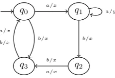
As a concrete example, we want to learn the functionLrepresented by the Mealy machine in the following diagram, where the input alphabet isI={a, b}
and the output alphabet isO={x, y}:
q0 q1
q2
q3 a/x
b/x b/x
a/y
a/x b/x a/x
b/x
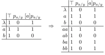
According to the algorithm 1, the first thing to do is checking if the starting table T = ({λ},{>}) is closed. The table is trivially closed, as>is always true and the first conjecture of the algorithm is as follows:
|λ| a/x b/x
As the conjecture is incorrect the teacher returns a counterexample, e.g. the formula [a]pa/y. We update the setΣof formulas with this new formula together
with all its subformulas. Note that this process is a well-known variant of the one described in [6] where the counterexample is usually added to the setS of states and not to Σ. We use this variant that allows to automatically maintain the table consistent (cf. [19]), in order to be sure to have a sharp table at every step.
The table is nowT = ({λ},{>, pa/y,[a]pa/y}) and it is not closed. Therefore,
[image:14.595.249.368.392.473.2]are not represented in S, in symbols:|Base(γ(x0))|Σ 6⊆ |S|Σ. In our particular
case, we can pick only λ; the two successors ofλare ha, xi andhb, xiand we have Base(γ(λ)) ={a, b}. We take one element of this set, saya, the equivalence class ofa is not equal to|λ|Σ, therefore we adda toS and we remove it from
Base(γ(λ)). We do the same forb. Because|b|Σ∈ |{/ λ, a}|Σ,b is also added toS.
This procedure can be seen as the standard table filling process in the L*-algorithm: in the lower part of the table, we identify those states that do not have a corresponding representative in the set of statesS and we add them in the upper part of the table; in our case both a andb have to be added. The entries of the table are 1 and 0, according to the truth values which the formula assumes in a particular state. We can schematically see this process in Table 1, where the values in the first column are shorthands for π1(γ(w)(a)), i.e., we
[image:15.595.218.397.310.404.2]writewafor the state reached fromwafter reading inputa.
Table 1.From a not closed table to a closed one
>pa/y [a]pa/y
λ 1 0 1
a 1 1 1
b 1 0 0
⇒
>pa/y[a]pa/y
λ 1 0 1
a 1 1 1
b 1 0 0
aa 1 1 1
ab 1 0 0
ba 1 0 1
bb 1 0 1
Having addedaandbtoS, we have a new table:T = ({λ, a, b},{>, pa/y,[a]pa/y}),
that is closed. Now, we can make our conjecture:
|λ| |a|
|b|
a/x
b/x
a/y
a/x
b/x a/x
b/x
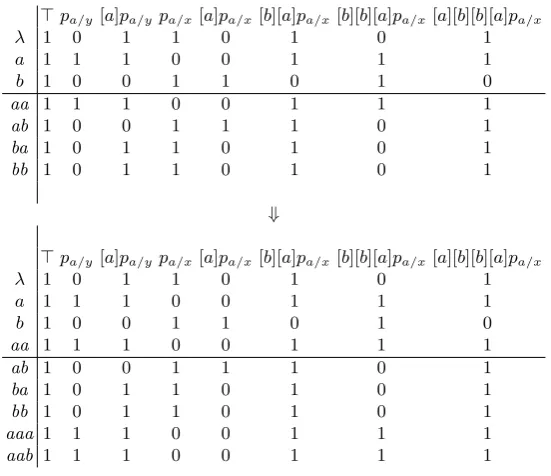
But the conjecture is incorrect and we again receive a counterexample, e.g. [a][b][b][a]pa/x. The resulting table is not closed, as|Base(γ(a))|Σ 6⊆ |S|Σ. Indeed,
the successor ofa,aa, should satisfy [a][b][b][a]pa/x, whereas the formula is false
ina. We only pick the elementaafrom Base(γ(a)) ={aa,ab}as the equivalence class ofab is already represented. The new table is:T = ({λ, a, b,aa}, Σ).
Closing the table withaa, we go toelse2 and we compute our conjecture. Table 2 on page 16 represents this step. No counterexamples are given back, therefore the conjecture is the right one and we have the same automatonAut(T) describing the Mealy machine we wanted to learn.
[image:15.595.248.366.450.530.2]Table 2.Changing of the table according to the Base-step of the algorithm
>pa/y [a]pa/y pa/x[a]pa/x[b][a]pa/x[b][b][a]pa/x[a][b][b][a]pa/x
λ 1 0 1 1 0 1 0 1
a 1 1 1 0 0 1 1 1
b 1 0 0 1 1 0 1 0
aa 1 1 1 0 0 1 1 1
ab 1 0 0 1 1 1 0 1
ba 1 0 1 1 0 1 0 1
bb 1 0 1 1 0 1 0 1
⇓
>pa/y [a]pa/y pa/x[a]pa/x[b][a]pa/x[b][b][a]pa/x[a][b][b][a]pa/x
λ 1 0 1 1 0 1 0 1
a 1 1 1 0 0 1 1 1
b 1 0 0 1 1 0 1 0
aa 1 1 1 0 0 1 1 1
ab 1 0 0 1 1 1 0 1
ba 1 0 1 1 0 1 0 1
bb 1 0 1 1 0 1 0 1
aaa 1 1 1 0 0 1 1 1
aab 1 1 1 0 0 1 1 1
the Mealy automata produce. This is not the case in our algorithm. The entries are always the values 1 or 0 according to the truth values of the formulas, whereas the output values are given by the functionγ.
Example 5 (Discrete Markov Chain).In this example we show that our algorithm can learn bisimulation quotients of (discrete) probabilistic transition systems. We confine ourselves to a finite example and we model probabilistic transition systems as PAt× Dω -coalgebras where At is a set of propositional variables
- in our example we will assume At = {p} for a single proposition p. Note, however, that the input model of our learning algorithm could be infinite and that our coalgebraic framework is general enough to cover a large variety of probabilistic systems [23]. Recall an expressive language for this example from Example 3. Consider now the following pointedPAt× Dω -coalgebra based on
X ={x0, x1, . . . , x6}with initial statex0and transition mapγ, where transitions
x0
x1
x2
x3
x4
x5 p
x6
0,1
0,2
0,4
0,3
0,7
0.3 1
0,8
0,2
1
0,9
0,1 1
The algorithm tries to learn a minimal pointed coalgebra that is behaviourally equivalent to (X, γ, x0). As always the algorithm starts with table ({x0},{>}).
This table is trivially closed and our first conjecture will be a state at which p does not hold and with a loop of probability 1. The teacher has to reject the conjecture and provides a counter example, e.g. the formula ϕ=L0.2L1p
as x0 |= ϕ and |x0| 6|= ϕ. This leads to the new table ({x0}, Σ1) with Σ1 =
{L0.2L1p, L1p, p,>}). We have Base(γ(x0)) ={x2, x3, x4, x6} and it is easy to
see that |{x2, x3, x4, x6}|Σ1 6⊆ |{x0}|Σ1. Therefore the table is not closed. It
can easily be checked that x2 ≡Σ1 x3 and x4 ≡Σ1 x6 and closing the table
leads to ({x0, x2, x4}, Σ1). We have Base(γ(x4)) ={x5} and obviously|x5|Σ1 6∈
|{x0, x2, x4}|Σ1 asx5 is the only state satisfying propositionp. Closing the table
we arrive at ({x0, x2, x4, x5}, Σ1) and this table is closed as readers can easily
convince themselves. The table leads to the correct conjecture:
|x0|
|x2|
|x4|
|x5| p
0,3
0,7
1 1
1
5
Conclusions
to provide an implementation in the near future. The biggest challenge will in our view be to implement a teacher that provides “good” counterexamples.
There are many more questions concerning our work that we would like to clarify: Our approach is currently very much based on the category of sets. This excludes for example the important example of linear weighted automata [2]. We believe that our arguments can be extended by (i) building on a duality between algebras and coalgebras and (ii) understanding how filtrations translate via this duality. There are some partial answers to the latter question in the modal logic literature (cf. e.g. [25, 26]) but modal logicians usually focus on properties of filtrations that do not play a role in learning. Closely related to this question is a more diagrammatic understanding of termination and correctness of our algorithm: we believe that all essential ingredients for this are contained in our work but we need to understand filtrations on a more abstract, categorical level.
References
1. Jacobs, B.: Introduction to Coalgebra: Towards Mathematics of States and Obser-vation. Cambridge Tracts in TCS. Cambridge University Press (2016)
2. Jacobs, B., Silva, A.: Automata learning: A categorical perspective. Volume 8464 of LNCS. Springer (2014) 384–406
3. van Heerdt, G.: An abstract automata learning framework. Master’s thesis, Radboud Universiteit Nijmegen (2016)
4. Moerman, J., Sammartino, M., Silva, A., Klin, B., Szynwelski, M.: Learning nominal automata. POPL 2017 (2017)
5. van Heerdt, G., Sammartino, M., Silva, A.: Learning automata with side-effects. CoRRabs/1704.08055(2017)
6. Angluin, D.: Learning regular sets from queries and counterexamples. Information and Computation75(2) (1987) 87 – 106
7. Ad´amek, J., Milius, S., Moss, L.S., Sousa, L.: Well-pointed coalgebras. Logical Methods in Computer Science9(3) (2013)
8. Gr¨adel, E., Thomas, W., Wilke, T., eds.: Automata, Logic, and Infinite Games. Volume 2500 of LNCS. Springer (2002)
9. Mac Lane, S.: Categories for the Working Mathematician. Volume 5 of Graduate texts in Mathematics. Springer-Verlag, New York (1971)
10. Jacobs, B., Rutten., J.: An introduction to (co)algebras and (co)induction. In: Advanced topics in bisimulation and coinduction. Volume 52 of Cambridge Tracts in Theoretical Computer Science. Cambridge University Press (2011) 38–99 11. Ad´amek, J., Trnkov´a, V.: Automata and Algebras in Categories. Kluwer Academic
Publishers (1990)
12. Cirstea, C., Kurz, A., Pattinson, D., Schr¨oder, L., Venema, Y.: Modal logics are coalgebraic. The Computer Journal54(1) (2009) 31–41
13. Kupke, C., Pattinson, D.: Coalgebraic semantics of modal logics: An overview. Theoretical Computer Science412(38) (2011) 5070 – 5094
14. Schr¨oder, L.: Expressivity of coalgebraic modal logic: The limits and beyond. Theoretical Computer Science390(2) (2008) 230 – 247
16. Desharnais, J., Edalat, A., Panangaden, P.: Bisimulation for labelled markov processes. Information and Computation179(2) (2002) 163 – 193
17. Kupke, C., Leal, R.A.: Characterising behavioural equivalence: Three sides of one coin. In Kurz, A., Lenisa, M., Tarlecki, A., eds.: Calco Proceedings, Berlin, Heidelberg, Springer Berlin Heidelberg (2009) 97–112
18. Blackburn, P., de Rijke, M., Venema, Y.: Modal Logic. Number 53 in Cambridge Tracts in Theoretical Computer Science. Cambridge University Press (2001) 19. Maler, O., Pnueli, A.: On the learnability of infinitary regular sets. Information
and Computation118(2) (1995) 316 – 326
20. Balle, B., Castro, J., Gavald, R.: Learning probabilistic automata: A study in state distinguishability. TCS473(2013) 46 – 60
21. Mao, H., Chen, Y., Jaeger, M., Nielsen, T.D., Larsen, K.G., Nielsen, B.: Learning probabilistic automata for model checking. In: 2011 Eighth International Conference on Quantitative Evaluation of SysTems. (2011) 111–120
22. Tzeng, W.G.: Learning probabilistic automata and markov chains via queries. Machine Learning8(2) (1992) 151–166
23. Sokolova, A.: Probabilistic systems coalgebraically: A survey. TCS412(38) (2011) 5095–5110
24. Gl¨uck, R., M¨oller, B., Sintzoff, M.: Model refinement using bisimulation quotients. In Johnson, M., Pavlovic, D., eds.: AMAST 2010. Springer (2011)
25. Ghilardi, S.: Continuity, freeness, and filtrations. Journal of Applied Non-Classical Logics20(3) (2010) 193–217