City, University of London Institutional Repository
Citation: Harder, F. and Besold, T. R. ORCID: 0000-0002-8002-0049 (2018). Learning
Lukasiewicz logic. Cognitive Systems Research, 47, pp. 42-67. doi:
10.1016/j.cogsys.2017.07.004
This is the accepted version of the paper.
This version of the publication may differ from the final published
version.
Permanent repository link: http://openaccess.city.ac.uk/19865/
Link to published version: http://dx.doi.org/10.1016/j.cogsys.2017.07.004
Copyright and reuse: City Research Online aims to make research
outputs of City, University of London available to a wider audience.
Copyright and Moral Rights remain with the author(s) and/or copyright
holders. URLs from City Research Online may be freely distributed and
linked to.
City Research Online: http://openaccess.city.ac.uk/ [email protected]
Learning Łukasiewicz Logic
Frederik Hardera, Tarek R. Besoldb
aFaculty of Science, University of Amsterdam, Amsterdam, The Netherlands bDigital Media Lab, Center for Computing and Communication Technologes (TZI),
University of Bremen, Bremen, Germany
Abstract
The integration between connectionist learning and logic-based reasoning is a
long-standing foundational question in artificial intelligence, cognitive systems, and
com-puter science in general. Research into neural-symbolic integration aims to tackle this
challenge, developing approaches bridging the gap between sub-symbolic and
sym-bolic representation and computation. In this line of work thecore methodhas been
suggested as a way of translating logic programs into a multilayer perceptron
comput-ing least models of the programs. In particular, a variant of the core method for three
valued Łukasiewicz logic has proven to be applicable to cognitive modelling among
others in the context of Byrne’s suppression task. Building on the underlying formal
results and the corresponding computational framework, the present article provides a
modified core method suitable for the supervised learning of Łukasiewicz logic (and
of a closely-related variant thereof), implements and executes the corresponding
su-pervised learning with the backpropagation algorithm and, finally, constructs a rule
extraction method in order to close the neural-symbolic cycle. The resulting system is
then evaluated in several empirical test cases, and recommendations for future
devel-opments are derived.
Keywords: Neural networks, Logic programs, Neural-symbolic integration, Cognitive
modelling, Reasoning
1. Introduction
Neural-symbolic integration attempts to bridge the gap between two prominent
ex-plicit knowledge representation, logic programming and search-based problem solving
techniques which have been responsible for many of the early successes in artificial
5
intelligence such as game playing, automated theorem proving and natural language
processing ([1, 2, 3]). While the paradigm is still very much alive in expert systems
managing and reasoning over vast quantities of symbolic data, it is also at times referred
to as “good old-fashioned AI” or GOFAI ([4]), having lost some of its appeal as its
lim-itations have become apparent. Learning from, and finding structure in sets of noisy
10
data is something symbolic AI largely fails at. Unfortunately this means that whole
classes of problems which are integral to a common conception of intelligence, such
as image and voice recognition, on a general scale currently can hardly be addressed
using symbolic AI.1Also, while (mostly non-monotonic) logic-based cognitive
mod-elling is still being pursued with valuable results, the brittleness of the corresponding
15
models together with their necessary restriction to high-level cognition (leaving out the
bigger part of the actual representation and processing apparatus of human cognizers),
are clear drawbacks when compared to connectionist or statistical approaches.
The second paradigm is that of machine learning. As the name suggests, it refers
to a variety of methods for learning from data, artificial neural networks (ANN)
be-20
ing one prominent group of these methods. Aided by a leap in processing power and
available data, machine learning has been credited with most of the more recent
ac-complishments in AI, from the now commonplace feat of handwriting recognition to
self-driving cars and the fully autonomous learning of computer games ([6, 7, 8]).
Promising as the paradigm may be, there are areas in which, on its own, it performs
25
very poorly. While the learning of simple logical dependencies from data is achieved
with relative ease, the process becomes increasingly difficult when higher order
cepts are involved ([9]). Examples for the latter impasse are numerous, including
con-nectionist systems’ problems with high-level visual analysis taking into account partial
1Recent logic-based approaches such as, for instance, Meta-Interpretive Learning for Logical Vision [5]
might in the future help to mitigate this problem, but currently have only reached proof of concept state
and still have to confirm their generalizability across tasks and domains, and their scalability to real-world
Figure 1: A conceptual overview of the neural-symbolic cycle (as introduced in [11]).
occlusion, light source identification, or shadow prediction, or with higher-level
infer-30
ence such as the recognition of intentions of depicted agents. Also, as knowledge is
represented in connectionist systems in a distributed fashion that is hard to interpret
from an outside perspective, it is usually difficult to provide background knowledge in
a format which the machine learning algorithm can use, or to extract learned features
from a network for instance for verification purposes. All of these are problems that
35
often become trivial when tackled with a symbolic system.
Much stands to be gained from a unification of the two paradigms that could cancel
out their respective weak spots and highlight their strengths. Neural-symbolic
inte-gration ([10]) offers some ideas in how this may be achieved, centering around the
concept of the neural-symbolic cycle (see Figure 1). The cycle contains two reasoning
40
systems. One is symbol-based, utilizing available expert knowledge, and the other is
a connectionist system or ANN, which learns from data. The challenge of interfacing
these systems is twofold. Coming from the symbolic side, the first task is to find a way
of translating the existing symbolic knowledge into the connectionist system, finding a
representation that is appropriate for the network. Secondly, one needs to devise
meth-45
ods for extracting the information gained by the connectionist system through learning
and convert it back into a clean symbolic format. Equipped with these processes of
representation and extraction the system as a whole is capable of incorporating both
background knowledge and training data as either become available.
When asked about the feasibility of integrating both paradigms, the human brain
50
struc-ture which operates on the basis of low-level processing of perceptual signals, but
cog-nition also exhibits the capability to efficiently perform abstract reasoning and symbol
processing; in fact, processes of the latter type are taken to provide the foundations
for thinking, decision-making, and other mental activities ([12]). It is precisely this
55
seamless coupling between learning and reasoning which is commonly considered the
basis for intelligence in humans—see also, e.g., [13], p. 163: “While I do not regard
intelligence as a unitary phenomenon, I do believe that the problem of reasoning from
learned data is a central aspect of it.”—and, in close analogy, quite plausibly also for the
(re-)creation of cognitive capacities up to human-level intelligence in artificial systems.
60
Returning to the neural-symbolic cycle discussed above, it should be made clear,
that the task of constructing such a cycle rapidly increases in difficulty when raising
the expressive capacities of the involved systems. There are approaches for fragments
of first order logic ([14, 15]), but most results focus on various propositional logics.
Furthermore, extraction algorithms for connectionist systems tend to be intractable. So
65
while the general method of the field can be described in a few pages, the underlying
problems are hard and there is still a long way to go before neural-symbolic integration
may be applied to state-of-the-art methods of either paradigm.
As one of the currently most prominent and best understood methods, H¨olldobler’s
and Kalinke’score method([16]) has since been developed as a neural-symbolic system
70
for, among others, propositional modal ([17]) and covered first order logic programs
([15]). It provides a way of translating logic programs into a type of multilayer
percep-tron (MLP) which, embedded in the core architecture, computes least models of these
programs. In [18], a variant of the core method for three valued Łukasiewicz logic is
presented, and it is suggested to apply the resulting approach to cognitive modelling
75
tasks (see, e.g., [19] for a subsequent application to Byrne’s suppression task [20]).
In the discussion of their work, the authors make the claim that the architecture they
have used can be modified in such a way, as to allow training via the backpropagation
algorithm ([21]). If this is in fact the case, when additionally equipped with a rule
ex-traction method, the resulting architecture should allow for a basic form of closure of
80
these ideas into practice by providing a modified core suitable for supervised learning,
implementing and executing supervised learning with the backpropagation algorithm
and, finally, constructing a rule extraction method. Section 2 gives an overview of the
85
theory and methods underlying this work, after which Section 3 is used for an in-depth
documentation of the implemented approch to learning cores and extracting learned
rules. We present the empirical results of the corresponding computational experiments
in Section 4, followed by a closing discussion and look ahead at future work in Section
5. The proofs corresponding to the theoretical results, together with the pseudo codes
90
of the extraction algorithm, have been relegated to the appendix.
2. Foundations
As conceptual basis for the work presented in subsequent sections, a number of
methods and terminology have to be clarified. The three following subsections will
respectively give a short introduction to Łukasiewicz logic programs, H¨olldobler’s and
95
Kalinke’s core method, and the backpropagation algorithm. Some basic familiarity
with classical logic and neural networks is assumed.
2.1. Łukasiewicz logic programs
We first introduce three-valued Łukasiewicz logic as a formalism, giving the main
definitions and a short account of key properties. Then we provide the relevant
infor-100
mation about logic programs and weak completion in the Łukasiewicz context, before
finally presenting the Stenning-van-Lambalgen consequence operator.
2.1.1. Three-valued Łukasiewicz logic
Łukasiewicz Logic was proposed in its ternary version in 1917 by Polish
philoso-pher and logician Jan Łukasiewicz ([23]), as a result of his work on modalities in logic.
105
The addition of a third value was meant to introduce a notion of possibility and
in-determinism to logical reasoning. Metaphysical import aside, this logic was the first
one to break with the true/false dichotomy of classical logic and thus lay the
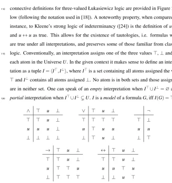
connective definitions for three-valued Łukasiewicz logic are provided in Figure 2
be-110
low (following the notation used in [18]). A noteworthy property, when compared, for
instance, to Kleene’s strong logic of indeterminancy ([24]) is the definition ofu→u
andu↔uas true. This allows for the existence of tautologies, i.e. formulas which
are true under all interpretations, and preserves some of those familiar from classical
logic. Conventionally, an interpretation assigns one of the three values>,⊥anduto
115
each atom in the UniverseU. In the given context it makes sense to define an
interpre-tation as a tupleI=hI>,I⊥i, whereI>is a set containing all atoms assigned the value
>andI⊥contains all atoms assigned⊥. No atom is in both sets and those assignedu
are in neither set. One can speak of anemptyinterpretation whenI>∪I⊥=∅and a
partialinterpretation whenI>∪I⊥(U.Iis amodelof a formulaG, iffI(G) =>.
120
∧ > u ⊥
> > u ⊥
u u u ⊥
⊥ ⊥ ⊥ ⊥
∨ > u ⊥
> > > >
u > u u
⊥ > u ⊥
¬
> ⊥
u u
⊥ >
→ > u ⊥
> > u ⊥
u > > u
⊥ > > >
↔ > u ⊥
> > u ⊥
u u > u
[image:7.612.114.458.115.482.2]⊥ ⊥ u >
Figure 2: Definitions of the connectives for three-valued Łukasiewicz logic.
As already mentioned in the previous section, according to H¨olldobler, Łukasiewicz
logic is of interest for modelling empirical observations of human reasoning.
Specifi-cally, [19] seeks to provide a logical model for the suppression task experiment ([20]).
In the corresponding set of experiments, Byrne analysed what conclusions readers will
typically draw from a certain class of natural language statements. As an example,
125
when reading the statement “If Marian has an essay to write, she will study late in
the library. She has an essay to write.”, 96% of all subjects concluded that “Marian
38% of participants conclude that Marian will indeed study in the library. It appears
130
that the additional information led more than half of the participants to revoke their
previous inferences, even though this information was not contradictory. The
non-monotonicity of this reasoning suggests that it cannot be modelled by classical logic.
Against this backdrop, in [19] it is therefore proposed that three-valued Łukasiewicz
logic interpreted under weak completion (as explained in the following subsection) fits
135
the findings best.2
2.1.2. Logic programs
Logic programs are defined as a finite set of clauses of the formA←B1∧B2∧. . .∧ Bnwhere the head of the clause,A, is an atom and theBi, with 1≤i≤n, in the body
are either literals,>or⊥. Clauses of the formA← >andA← ⊥are calledpositive 140
andnegative factsrespectively.
These logic programs are interpreted under weak completion, which takes a logic
program and transforms it into one single formula, thereby changing how it is
evalu-ated. Firstly, the bodies of all clauses with the same head are concatenated as a
disjunc-tion into one body. After this step, the resulting formulas consist of one implicadisjunc-tion
145
per head. Subsequently, all←are replaced with ↔. As a result, atoms which are
heads in clauses whose bodies all evaluate as⊥are now⊥as well. Finally,
concate-nating all clauses into one conjunction creates a single formula representing the weakly
completed program.
Weak completion adds non-monotonicity to Łukasiewicz logic. Atoms which
eval-150
uate as⊥because all associated bodies evaluated as⊥, can become>when adding
another clause without contradiction. Also, weakly completed Łukasiewicz logic
pro-grams are never contradictory, always having at least one model ([18]).
2There is an ongoing controversy on whether Łukasiewicz logic under weak completion, or completion
semantics based on the three-valued logic used by Fitting [25], is better suitable for modelling human
rea-soning in general, and the suppression task in particular. While this debate and its eventual solution are
of general interest, in this article we stay agnostic concerning the matter. Instead, as stated at the end of
Section 1, the aim is to equip the system from [18] with a backpropagation-trainable type of core and a rule
2.1.3. Consequence operators
Models for such a logic programPcan be computed through a consequence
op-155
eratorΦP. Starting from an empty interpretationI, the immediate consequenceΦP(I)
is calculated as a new interpretation and this process is iterated, untilI=ΦP(I)and
a fixed point is reached. It can be shown ([18]) that the least models of Łukasiewicz
logic under weak completion are identical to the least fixed points of the
Stenning-van-Lambalgen consequence operatorΦSvL,Pfrom [26], which is defined as follows: 160
ΦSvL,P(I) =hJ>,J⊥i, where
J>={A|∃(A←body)∈P:I(body) =>}and
J⊥={A|∃(A←body)∈P∧ ∀(A←body)∈P:I(body) =⊥}
The next section discusses the algorithm introduced by [18], which translates the
ΦSvL,Pconsequence operator of a given program into a 3-layer feed-forward network, 165
that computes the same function. Like the consequence operator, this network may
then be used on multiple iterations until a fixed point is reached.
2.1.4. Example: consequence operator application
In order to illustrate, how the consequence operatorΦSvL,Pfunctions, we provide a
small example. Consider the following four clauses:
170
A← ⊥
B← ¬A
C← ¬B
C←B∧ ¬C
All literals default touin the beginning. The first application of the consequence
operator adds A toJ1> following the first clause. The bodies of clauses 2,3 and 4
evaluate asuand nothing else happens. The second application,ΦSvL,P(I1), finds clause
as⊥, but the body of clause 4 is stillu, and as a result, a fixed point is reached. The
175
sequence of interpretations is given in the table below.
I0 I1 I2 I3
A u ⊥ ⊥ ⊥
B u u > >
C u u u u
2.2. The core method
In the following, a detailed description of how the core architecture is set up will
be provided. This account chooses a somewhat different perspective than that of the
translation algorithm given in [18]. While the algorithmic description is optimal for
180
implementation, the angle used here will hopefully provide a better understanding of
the core structure with regard to the modifications that must be made to it, and to the
introduction of sigmoidal activation units in particular.
In both input and output layer of the network, each atomAof the program is
repre-sented by two neurons. Activation in the first one indicatesA=>, while activation in
185
the second one meansA=⊥. If neither neuron is active, thenA=u. The core does not
allow for both neurons to be active in the same iteration. The input layer also contains
one neuron each, representing>and⊥, which are always active. Each program clause, or rather each clause body, is represented by two neuronshh>,h⊥iin the hidden layer. Whether a clauses body is mapped to>,⊥oruis encoded in the same way as was
190
used for the atoms.
All connections between the layers of the core serve the function of logic gates. An
h>neuron is connected to one input layer neuron for each conjunct in the clause body
it represents. If the conjunct is an atomA, it connects toA>, if it is a negated atom¬A,
it connects toA⊥and if the conjunct is>, it connects to that unit. Connection weights
195
and activation threshold are set to form an ’and’-gate, requiring activation of all input
layer neurons for the clause neuron to fire. In case a conjunct is⊥, no connection is
formed, but for sake of the logic gate this is treated as a connection to an inactive unit,
A⊥neurons, whereAis a conjunct andA>neurons, where¬Ais one. If⊥is a conjunct,
200
h⊥connects to the⊥neuron and if>is a conjunct, no connection is formed. Weights
and threshold are set to form an ’or’-gate, such thath⊥is activated when one or more
input neurons fire. This way, clause bodies are represented as>if and only if all their
conjuncts are mapped to>and represented as⊥, if and only if one or more conjuncts
are⊥.
205
In the output layer, each neuron has one connection for each clause in which the
associated atom appears as head. A> neurons are connected to the h> neurons of
the associated clauses, forming an ’or’-gate andA⊥neurons are connected to theh⊥
neurons, forming an ’and’-gate. Thus atoms are>when one or more associated clauses
are>, and⊥, when all associated clauses are⊥.
210
The logic gates are implemented such that all connection weights in the network
have the same value ω>0 and ’or’-gate thresholds are at 0.5·ω, while ’and’-gate thresholds equal to(l−0.5)·ω, wherel is the number of incoming connections. All neurons use the Heaviside activation function, emitting 1, if the received activation
meets or exceeds the threshold and 0 otherwise. Given this setup, computing a fixed
215
point merely involves feeding the network’s output back into the input layer until it
equals the previous output3.
2.2.1. Example: core method computation
For an example of how this core works in practice consider the four clauses used
in the previous example:A← ⊥,B← ¬A,C← ¬B,C←B∧ ¬C. Application of the
220
translation algorithm yields the following multilayer perceptron.
3The number of iterations necessary for reaching the least fixed point can be shown to be lesser or equal
to the number of atoms. The network has no inhibitory connections, so more input always generates equal
or more output. Starting from an empty interpretation, each subsequent iteration must therefore activate at
A> A⊥ B> B⊥ C> C⊥
> ⊥
A> A⊥ B> B⊥ C> C⊥
h>1 h⊥1 h>2 h⊥2 h>3 h⊥3 h>4 h⊥4
The following figures show how activations propagate through the network on each
iteration, starting in the input layer at the bottom. Red arrows and grey cells indicate
active connections and units. As before, a fixed point is reached after three steps.
225
A> A⊥ B> B⊥ C> C⊥
> ⊥
A> A⊥ B> B⊥ C> C⊥
h>1 h⊥1 h>2 h⊥2 h>3 h⊥3 h>4 h⊥4
The first iteration starts off with >and ⊥, the latter of which activates the h⊥1
neuron, which, being set as an ’or’-gate, has a threshold of 0.5 and this in turn activates A⊥in the output, because the ’and’-gate with a single clause also has a threshold of
0.5.
A> A⊥ B> B⊥ C> C⊥
> ⊥
A> A⊥ B> B⊥ C> C⊥
h>1 h⊥1 h>2 h⊥2 h>3 h⊥3 h>4 h⊥4
The Second iteration then starts withA⊥active and this activatesh>2 andB>in the
output.
A> A⊥ B> B⊥ C> C⊥
> ⊥
A> A⊥ B> B⊥ C> C⊥
h>1 h⊥1 h>2 h⊥2 h>3 h⊥3 h>4 h⊥4
On the third iteration, the now activeB>input unit activates theh⊥3 unit, but does
235
not activateh>4, as the ’and’-gate has a threshold of 1.5 and the second incoming con-nection fromC>is not active. theC⊥unit in the output also has a threshold of 1.5 and does not activate. At this point the output equals the input, not taking into account the
auxiliary>and⊥units, and a fixed point is reached.
2.3. The backpropagation algorithm 240
The backpropagation algorithm, introduced in [21], has become the probably most
widely used training algorithm for feed-forward networks. It offers a computationally
efficient way of deriving the partial derivatives of the cost function for classification
for adjusting the weights, usually through gradient descent, so the cost function is
min-245
imized. The name backpropagation derives from the order in which the partial
deriva-tives are calculated. This process begins in the output layer and propagates backward,
layer by layer, as the calculation in each layer requires the results of its successor.
The derivation of the backpropagation algorithm is fairly general and holds for
dif-ferent cost and activation functions. Given the binary nature of the targets, we choose
250
the logistic cost function4, because it encourages binary output. As activation
func-tion, the standard sigmoid is used. The specific formulas used in the algorithm depend
on the choice of function. A derivation for the algorithm with quadratic loss function,
along with a general introduction to the algorithm, can be found in [27] and an
analo-gous derivation for the backpropagation that was used here is provided in the appendix.
255
The implementation uses on-line training, which means that weights are updated
ev-ery time after calculating the error for one randomly selected sample. The advantage
of on-line learning over batch training for our purposes is that the former better
ac-commodates the large variations in sample size that are encountered in different cores.
Aside from this, the choice is of no conceptual importance.
260
Additionally, in our experimental implementation the na¨ıve backpropagation
algo-rithm has been enhanced by using a momentum term, saving the weight adjustment
terms in each iteration and adds a fraction of them to the weight adjustment in the next
iteration. This tends to speed up convergence by preventing fluctuation of the weights
to some extent and also leads to some robustness against small local optima. Since
265
we focused on qualitative rather than quantitative results, this is the only significant
modification to the original algorithm. Where a consistent, if limited, level of learning
success can be shown with our basic implementation, it is plausible to assume that
fur-ther attempts with more sophisticated versions of the learning algorithm (also
includ-ing, for instance, techniques such as regularization, linear-least-squares initialization,
270
or simulated annealing) will yield much better results.
4J(~w) =1
m∑ m
i=1[(y(i)logh~w(x(i)) + (1−y(i))log(1−h~w(x(i)))], with~wthe vector of weights andh~w(x(i))
3. Theory and implementation of learning cores
We now document the theoretical groundwork and the actual implementation which
have gone into this project, beginning with modifications made to the core architecture,
followed by some remarks on the learning algorithm and a thorough discussion of the
275
proposed rule extraction algorithm. The section closes with a list of control measures
used in the implementation.
Before supervised learning can be attempted in cores, three problems have to be
addressed:
1. The core architecture must reach fixed points to compute results. While the
ex-280
istence of these fixed points has been proven for translated programs, this result
does not generalize to cores whose weights have changed over the learning
pro-cess. The first task, therefore, is to ensure the existence of fixed points throughout
the learning process.
2. Following the example given, for instance, in [28], a differentiable activation
285
function must be introduced, while preserving the core’s semantics. The
back-propagation algorithm relies on the computation of derivatives of the cost
tion which includes the activation functions of the network. The Heaviside
func-tion is not differentiable and must be replaced.
3. One must decide, what kinds of samples will be used for supervised learning.
290
The core in its original form is only capable of computing the least fixed point,
when starting from an empty interpretation. If one wants to capture any of the
structure of the program, more than one sample is needed for training.
The following subsections address these issues in turn, before drawing all the
indi-vidual steps and solutions together in a backpropagation algorithm for learning cores.
295
The second to last subsection then introduces the rule extraction algorithm, before the
final subsection shortly touches upon two measures introduced in order to assure the
3.1. Ensuring a fixed point with unipolar weights
Convergence to a fixed point is essential to the core method. While this
prop-300
erty is guaranteed for H¨olldobler’s and Kalinke’s discrete cores and will be proven for
their sigmoidal analogs below, it is difficult to ensure it throughout the learning
pe-riod, where the network may change drastically and with little regard for the structure
in which it is embedded. Convergence, therefore, should be guaranteed by something
other than the initial setting of the weights. A possible solution to this issue, and the
305
one employed here, is to restrict the network to unipolar weights. When limiting all
non-bias weights to positive values, there are no inhibitory connections and thus the
ac-tivation of the network will monotonically increase on every iteration until it plateaus
at a fixed point. On the downside, the elimination of inhibitory units of course reduces
the modelling capacity of the network. The reason it can nonetheless be done in good
310
conscience here, is that the translation of logic programs into cores itself only uses
pos-itive weights and thus ensures that every Łukasiewicz logic program to be learned by
a core can be fully modelled, and therefore also learned, using these simpler unipolar
networks.
A standard activation function used in feed forward networks is the sigmoid
func-315
tionsig(z) =1/(1+e−z)where z=~wT~x, the dot product of the weight vector and the incoming activations. In the implementation of unipolarity is achieved by squaring
all but the bias weight in the activation function. So, while the sigmoid function
re-mains the same,zis now computed asw0·x0+∑i>0(12(wi)2·xi). The values stored in
the weight matrix may still be negative, but will effectively be treated as positive. To
320
preserve the previous behaviour of cores, all non-bias weights are replaced by their
re-spective square root after the translation algorithm has been applied. With this measure,
the translation algorithm can ignore the modification to the activation function and act
as if it was the standard sigmoid, so long as it only sets positive weights. The
subse-quent argument that semantics are preserved in the sigmoidal core will also assume the
325
3.2. Preserving core semantics
With the introduction of sigmoidal activation to the network, the range of
possi-ble activations for each neuron changes from 0 and 1 to the interval]0,1[, and what it means for a neuron to ’fire’ becomes less clear. To ensure compatibility with the
330
core architecture, the network’s output is discretized by rounding it half up to 0 and 1.
A fixed point is reached when this rounded output is equal to the input of the current
iteration. Whithin the network, however, instead of an activation value it makes more
sense to define an interval bounded by a certain value[A+,1]where all activation val-ues in that interval are considered as firing, and another interval[0,A−]of activations
335
regarded as not firing.
As these two intervals should be disjoint, it follows thatA−<A+and because the classification into firing and non-firing is integral to the way the core is built, it must be
ensured that no activations in the interval]A−,A+[are produced. Given these changes, the approach of using logic gates, which was explained in the previous section, can
340
be maintained, but must deal with the following complications. Because the output
of a non-firing neuron is no longer 0, and can take on values up toA−, an ’or’-gate
must ensure that it won’t fire, even if all connected neurons send an activation ofA−
each, while at the same time guaranteeing that it will fire if one neuron sends activation
A+and all others send nothing. Similarly ’and’-gates should fire when all connected
345
neurons from the previous layer send A+, but not if all but one send an activation
of 1 and the last one sendsA−. It becomes clear that these constraints of maximal
non-activating input and minimal activating input5can only be satisfied with the right
choice ofA−andA+. In the core, bothA−andA+ are determined by the value of
ω. If ω is large, A− andA+, approach 0 and 1 respectively. For a smallω, both
350
values lie close to 1/2. It can be shown, that semantics of the network are preserved ifω>2 log(2deg−1), wheredegis the maximum in-degree among neurons in the output layer. The formal proof for this can be found in the appendix.
3.3. Fixed point calculation with initial activation
The original core architecture serves to compute fixed points for a given logic
pro-355
gram and no additional input. Evidently, this one sample of (empty) input and
cor-responding output does not contain exhaustive information about the program which
produced it. To train a network which captures the functionality of the program, more
samples are required. Given the context of logic programs, it seems like an obvious
choice to generate additional samples for possible interpretations of the atoms. There
360
are 3npossible interpretations for a set of ternary logic formulasPwithnatoms. What
additional inferencesPallows, based on a partial interpretation, provides information
aboutP, and having this information for all 3ninterpretations specifiesPto its semantic
equivalence class.6
3.3.1. C-interpretation 365
A na¨ıve approach for using such partial interpretations in a core is to enforce them
as the base activation while running the core, and see what additional inferences are
drawn before reaching a fixed point. This is achieved by adding the interpretation to
every starting activation on the first iteration as well as to the output at the end of
every iteration. This method must be called na¨ıve because the underlying definition of
370
interpretations, while applicable to Łukasiewicz logic, actually makes very little sense
for the weakly completed logic programs at hand. Determining the value of an atom
from the outset, while leaving the program as is, takes away both the non-monotonicity
and the property of non-contradiction. On the plus side, only few changes to the core
are necessary to accommodate this interpretation, which will from now on be referred
375
to as C-interpretation.
3.3.2. Ł-interpretation
In order to preserve the semantics of weakly completed Łukasiewicz logic, an
al-ternative Ł-interpretation is proposed. Here the process will be handled slightly
differ-ently, as it seems more adequate to model different interpretations in such a way that
380
6If the interpretation leads to no contradictions, it is a model ofP, otherwise it is not. Knowing all
they represent logic programs in their own right. As such, setting an atomAto>or⊥
in the interpretation should have the same effect as adding a positive or negative fact
to the program. Doing this preserves the important property, that the
Stenning-van-Lambalgen consequence operator always reaches a model. Note that in this choice of
interpretation setting atoms to false only has an effect, if they do not occur as heads of
385
clauses in the program, and that setting atoms to true in the interpretation will prevent
the consequence operator from inferring these atoms to be false even if all other clauses
in the program would lead to this conclusion.
Going with the interpretation as adding clauses to the program, the most intuitive
approach would be adding neurons to the hidden layer of the core which represent these
390
rules. Unfortunately this does not seem like a viable option. The addition of neurons
would change the in-degrees of some of the core’s output units which would in turn
necessitate an update of their respective bias weights, in order to maintain Łukasiewicz
semantics. For each interpretation there could be changes to the whole network which
would not only be computationally costly but also pose problems in the context of
395
learning, where changes to the core network should likely be limited to the learning
algorithm itself.
Instead it appears more promising to adjust the way in which the inputs to the
network are generated and outputs are interpreted. For negative facts likeA← ⊥this
is can be done fairly simply. Given weak completion these clauses only affect the
400
program at all, if there is no other clause with headAin the program. In this caseA
will be set to⊥and keep this value, as there is no other clause to change it. This can
be modelled in the core by checking the in-degree of the atom’s associated output unit
in the network. If the in-degree is 0,Ais set to⊥in the input to the network on every
iteration as well as on the final output, which in the neural net means the activation
405
of the neurons corresponding toAis(0,1). Positive facts of the typeA← >have to be treated differently. If such a clause exists,Awill be true independently of the rest
of the program. This meansAshould be set to >on all inputs as well as the final
contradiction must be resolved and the easiest way of doing this is to set activation of
theA⊥neuron in the output to 0 on all inputs and the final output.
3.3.3. C*-interpretation
In addition, a form of Ł-interpretation will be tested, which is different only in that
415
it leaves out the contradiction resolution step. The resulting new C*-interpretation can
be viewed as using explicit negation, rather than the negation by failure present
un-der Ł-interpretation, with regards to elements of the interpretation. Unfortunately, this
makes the logic monotonic and allows for contradictions. C*-interpretation is
nonethe-less of interest because, as will become obvious from the results reported below, it can
420
be trained better than Ł-interpretation but still bears some similarities. Training
un-der C- and C*-interpretations performs so similarly that C-interpretation will not be
discussed separately in the empirical results.
It is clear that all three interpretations generate the same output for empty
inter-pretations. Furthermore it can be shown, that all non-contradictory models under
C*-425
interpretation are equivalent to the Ł-interpretation under the same input7. All three
interpretations have been implemented and tested.
3.4. Backpropagation in cores
With the modifications to the core that have been described above it is now possible
to create samples and test the core’s capacity for learning. In the given set-up, two cores
430
are used. The first core is generated by translating the complete program into it and is
subsequently run with all possible inputs computing the desired outputs, the pairs of
which will be used as training samples. Core number two is created based on a partial
version of the program, where some clauses have been deleted. The learning task now,
is to train the second core with samples from the first one and see whether it can learn
435
the missing parts of the program.
It may take the core multiple iterations to reach a fixed point, but only the last one
is used for training. For a given sample, the core is run on the sample input and when
reaching a fixed point returns activation values of all the networks layers. Note that
the activation of the output layer is not the final output of the core, which may contain
440
modifications from interpretation or contradiction-resolution. The backpropagation
al-gorithm is then applied to the network with that activation. Due to the non-classical
activation function used in the network, the algorithm differs slightly from its more
common form. The derivation of the relevant formulas found in the appendix is done
analogous to the proof of standard backpropagation found in [27].
445
3.5. Rule extraction
The algorithm for extracting information from a core discussed in this section
fo-cuses on C- and C*-interpretation. It has been pointed out previously that through
iterations the core’s activation increases monotonically under these interpretations, due
to a lack of inhibitory connections in the network. The same reasoning ensures
mono-450
tonicity with regard to interpretations. While the number of possible interpretations
rises exponentially with the number of atoms, diminishing hopes for a tractable rule
extraction algorithm, the property of monotonicity allows for heavy pruning, making a
viable solution at least for small sample sizes possible.
Our algorithm is inspired by the approach for knowledge extraction and the
corre-455
sponding algorithm for regular networks from [29]. Still, the method presented here
warrants an independent introduction as well as analysis for soundness and
complete-ness.
3.5.1. The basic extraction algorithm
The algorithm extracts all minimal activating and all maximal non-activating inputs
460
for each output neuron of the network, which can then be used to compute the logical
rules generating this activation. In the following, the set of all inputs to the network
will be looked at as a partial order with the input vector of zeros as bottom element
and the vector of ones as top element. Input vectors are ordered in such a way that
v1≥v2⇔ ∀i:v1[i]≥v2[i]. 465
For each output neuron separately, the algorithm traverses the space of all possible
interpre-tations starting from top and bottom element. The new boundaries are generated by
computing alldirect successorsof each element of the existing boundary. For an
el-ement of the lower boundary a direct successor is a copy of the elel-ement in which
470
exactly one activation is changed from 0 to 1. The direct successor of an element in
the upper boundary, analogously, has one active input less than that element. All
in-puts connected through a series of direct successions will be called successors and the
definition for predecessors follows from this. An input in the lower boundary is said to
besubsumedby an activating input if it is a successor of that input and is subsumed by
475
a non-activating input, if it is a predecessor of that input. For subsumption in the upper
boundary, successor and predecessor relations are reversed. In either case, the
target-activation produced by the subsumed input is equal to, and therefore determined by, the
other input. Whenever an activating input is found in the lower boundary, which is not
subsumed by an input already stored in the set of minimal activating inputs, it is added
480
to that set. The progression through a lower boundary ensures that all predecessors
have already been checked and the one that has been found is in fact minimal. Also,
if all direct successors of a non-activating input are activating, then that input is added
to the list of maximal non-activating inputs. In the upper boundary, relevant inputs are
found in an analogous manner, where activation is the default. The algorithm
termi-485
nates once the two boundaries have passed by one another, which is not implemented
explicitly, but a result of the pruning mechanisms discussed below.
Prior to pruning, the soundness and completeness of the extraction algorithm are
evident, but spelled out here for the sake of completeness. All activating inputs found
in the lower boundary, which are not greater than previously found ones are minimal,
490
as all smaller activating inputs would be in that set. Complementary, all non-activating
inputs whose direct successors are activating are maximal, as all their successors are
activating due to monotonicity. The analog holds for the upper bound. Thus the
ex-traction is sound. All minimal activating inputs are found by the algorithm, as they are
activating and not subsumed by any other activating inputs. All maximal non-activating
495
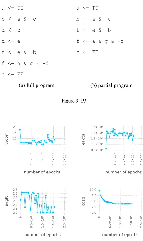
inputs are found by the algorithm as the successors of each are activating by definition.
Here, too, the analog is true for the upper bound and so the extraction is complete as
3.5.2. Pruning
Due to the monotonic nature of the space of possible inputs, once an activating
500
input is found in the lower bound, none of its successors need to be investigated any
more, as all of them will be activating as well. An efficient extraction algorithm must
therefore limit its exploration of the space of possible inputs to the relevant nodes which
may hold new information. The pruning is best explained from the perspective of one
of the boundaries. From the perspective of the lower boundary, minimal activating
505
inputs will be calledrulesand maximal non-activating inputs are calledanti-rules(for
lack of a better term). These terms are relative to the boundary, such that rules in the
lower boundary are anti-rules in the upper boundary and vice versa. When a rule is
discovered, all of its successors should be pruned, as their values will hold no new
information. This must be ensured both in the current boundary, where it is a rule,
510
and the opposite boundary, where it is an anti-rule and two pruning mechanisms ensure
this.
The pruning mechanisms can not be explained without covering the specifics of the
algorithm in some detail. It may help to have a look at the pseudo code provided in the
appendix for reference.
515
To avoid too much confusion, the algorithm refers to inputs as vertex objects, owing
to the graph-like feel of the partial order. Alongside its input value and a number of
other things, each vertex stores a memory array to keep track of the direct successors
it should generate and those that should be pruned. This array has one entry for each
neuron, which is 1, if switching the value of this input from 0 to 1 or vice versa will
520
generate a valid successor, 0 if the successor and all subsequent successors are invalid,
and -1 if the direct successor is invalid, but later ones may be valid.
Thetest function checks whether a vertex is a rule or subsumed by an anti-rule.
If the vertex is a rule, the memory array is set to all zeros, so that no successors are
generated and the vertex is added to the set of found rules. If the vertex is subsumed
525
by an anti-rule, some, but not necessarily all successors will be subsumed as well. In
all places where switching the input would generate a subsumed direct successor, the
This information is utilized in thesuccessorsfunction. As the name suggests, this
function creates the direct successors of a given vertex, but also uses the step to
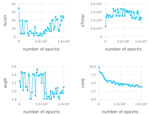
ex-530
change pruning information among the successors. Firstly, the input vertex istested
again, in case new anti-rules were discovered while traversing the other boundary.
Then, each valid direct successor of the vertex (as indicated by the memory array) is
looked up and if it does not exist yet, is generated and tested. For each such successor
which is a rule, the preceding vertex’s memory is set to 0 at the index, which was used
535
to generate that successor, indicating that this successor should not be investigated
fur-ther. After this has been completed, all the successors are traversed for a second time
and all 0s from the vertex memory are copied into their respective memories as well.
This way, each successor receives information about all vertices, with which it shares
a common direct predecessor. Now, when a rule is discovered, all of its direct
prede-540
cessors will set the index in their memory which generated this rule to 0 and pass this
information on to all their successors. If a vertex subsumed by the rule were to be
gen-erated, it would have to have a direct predecessor which is not subsumed by the rule (or
the problem propagates down until this condition occurs). This predecessor, however,
must be a successor of one of the rule’s predecessors. Therefore it would not generate
545
that vertex and it follows that no vertices subsumed by rules are generated. Note that
the same does not hold for anti-rules. Finally, the successors function also serves to
determine, whether the given vertex is an anti-rule. This is the case, if the vertex is not
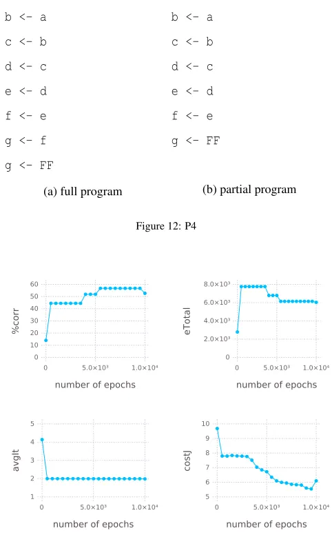
subsumed by an anti-rule (i.e. no entry in the memory is set to−1) and no generated
successor has the same target-activation value as the vertex. As rules trivially share
550
these properties by having all their successors pruned, they must be filtered out. This
is done by checking for the right target-activation, given the vertex’s boundary, before
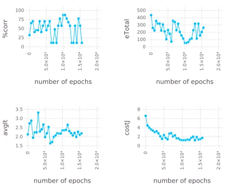
adding it to the set of rules. In the lower bound an anti-rule must be non-activating,
and activating, if in the upper bound. So now, when therules for targetfunction
fi-nally creates the two boundaries and traverses the partial order, the pruning ensures no
555
vertices that are subsumed by known rules are looked at.
The anti-rule related pruning is handled with some care by the algorithm, as it can
lead to problematic cases. In general, it might happen, that all direct successors of a
succes-sors invalid could hinder the generation of valid ones down the line. If, for example,
560
(1,1,1,1,0,0,0)and(1,0,0,0,1,1,1)were known anti-rules, the lower boundary in-put(1,0,0,0,0,0,0)would generate no direct successors and unsubsumed successors like(1,0,0,1,1,0,0)would not be reached. In the algorithm this problem is solved by looking only at the first anti-rule found, rather than the whole set of subsuming
anti-rules. Apart from the trivial case where the anti-rule is the top or bottom element
565
(which ends the search as either all inputs are activating or none are), a single anti-rule,
will not prune all successors of the vertex. The indices at which the anti-rule differs
from its predecessors (of which, barring the trivial cases, it has at least one) can be
changed in the vertex to generate valid successors.
Of course this strategy can, at times, dismiss useful information and generate
ver-570
tices which are subsumed by known rules at the point of creation. As a stand-in for
more elaborate methods it will suffice to generate some first results.
In order to ensure that soundness and completeness are maintained, it must be
proven that pruning neither changes the results of examining a particular vertex, nor
prevents any rule vertices from being examined. Addressing part one, the test for rules
575
functions in the same way as without pruning and only relies on the vertex’s target
activation value, which is not affected by pruning. With pruning, the test for anti-rules
employs the memory of the given vertex, rather than looking at all successors, but it
does so, only to infer the target-activation values of the invalid immediate successors.
Assuming that rules have been identified correctly, every 0 in the memory is linked to
580
a successor which has a different target-activation value than the vertex. Each−1 is
linked to a successor which has the same value as the vertex. Generating each of these
invalid successors would take more time but yield the same result. Therefore all
exam-ined vertices are still classified correctly. The second part follows from the soundness
of the pruning algorithm.
585
3.5.3. Example: rule extraction
As an illustration of the extraction algorithm, we consider a network with only two
>and⊥unit of a literal are active.
590
uA,uB
>A,uB ⊥A,uB uA,>B uA,⊥B
EA,uB >A,>B >A,⊥B ⊥A,>B ⊥A,⊥B uA,EB
EA,>B EA,⊥B >A,EB ⊥A,EB
EA,EB
The extraction algorithm is applied for each of the four units (A>,A⊥,B>, B⊥)
separately. We begin by looking at A>. Memory cells of highlighted elements are
encoded as a 4-tuple, which indicates changes to the units in the same order. So,
for example, element(>A,uB) with memory[0,1,0,1] will generate the successors 595
(EA,uB)and(>A,⊥B).
uA,uB
>A,uB ⊥A,uB uA,>B uA,⊥B
EA,uB >A,>B >A,⊥B ⊥A,>B ⊥A,⊥B uA,EB
EA,>B EA,⊥B >A,EB ⊥A,EB
EA,EB
[1,1,0,1]
[0,1,0,1] [1,0,0,1] [0,0,0,0] [1,1,0,0]
Starting at the bottom element, we find that zero activation in the input does not
activateA>. Going through the four immediate successors,(>A,uB)and(⊥A,uB)both
turn out as non-activating inputs and are queued up for the following iteration. Then
600
(uA,>B)is tested and turns out to be a minimal activating input, i.e. a rule, and the
memory of the bottom element is adjusted accordingly from[1,1,1,1] to[1,1,0,1]. After testing(uA,⊥B) and adding it to the queue as well, the memory of the three
uA,uB
>A,uB ⊥A,uB uA,>B uA,⊥B
EA,uB >A,>B >A,⊥B ⊥A,>B ⊥A,⊥B uA,EB
EA,>B EA,⊥B >A,EB ⊥A,EB
EA,EB
[0,1,0,1] [1,0,0,1] [0,0,0,0] [1,1,0,0] [−1,−1,0,−1]
[0,0,0,0]
605
The second element in the queue is the top element, which activatesA>upon testing
is therefore not a rule of the upper bound. It is, however, subsumed by the newly
discovered anti-rule(uA,>B)and the element’s memory is updated to[−1,−1,1,−1]
to reflect this. As a result, three of the four direct successors are pruned. The fourth
one, (EA,⊥B), is generated, queued and tested. It turns out to be a maximal non-610
activating input and thus an upper boundary rule. The top element’s memory is updated
to[−1,−1,0,−1]and this update is passed to all its successors, which has no effect in this case.
uA,uB
>A,uB ⊥A,uB uA,>B uA,⊥B
EA,uB >A,>B >A,⊥B ⊥A,>B ⊥A,⊥B uA,EB
EA,>B EA,⊥B >A,EB ⊥A,EB
EA,EB
[0,−1,0,−1] [−1,0,0,−1] [0,0,0,0] [−1,−1,0,0] [0,0,0,0]
Next, the four queued lower boundary elements are tested. One is the lower bound
615
rule and the three others are all subsumed by the anti-rule(EA,⊥B), and after updating
their memories, no new successors are queued. Finally, the upper bound rule is taken as
a last element from the queue, producing no successors, and the algorithm terminates.
3.6. Controls
Verifying the correctness of an implementation as a whole beyond the checking of
test cases is usually associated with an enormous effort and has therefore not been in
the scope of this project. Checks have been installed at two crucial steps in the program
which are worth mentioning:
625
1. A function has been implemented which can run a core with discrete activation
units as in the original algorithm (with the one difference that it squares all
non-bias weights to compensate for the fact that they were reduced to their square
roots in the new translation). The function is used to run a core with both kinds
of activation and for all possible inputs under a chosen interpretation, returning
630
an error if the activations reach different models for the same input. This way,
it is possible to verify that the implementation of the translation algorithm with
sigmoidal units does preserve the semantics of the cores.
2. As a standard measure to ensure the correctness of the implementation of the
backpropagation algorithm, numerical gradient checking has been implemented.
635
As gradient checking is computationally costly, it is only used on a small number
of training samples to verify the correctness of backpropagation and disabled
for the actual training of the network. Given the more complicated nature of
learning in a core as compared to the classical application of backpropagation
there are a number of other errors that may occur which prevent learning and are
640
not detected by gradient checking, but the method still serves to eliminate one
common source of errors.
4. Empirical results
Test following test results are based on an implementation in Julia.8 The source
code of our implementation is open source and available for download from GitHub.9As
645
already stated before, a thorough quantitative analysis of training results is not within
8julialang.org
the scope of this article. Instead, several exemplary cases will be used to highlight
consistently observed features of the learning process.
The first such program is displayed below in the format, in which it is read by the
implementation. To keep things simple and in ASCII-encoding,←,∧, and¬have been
650
written as<-,&and-respectively. The partial program, consisting of clauses 1, 5 and
6, is translated into a core and then trained on samples generated from the full program.
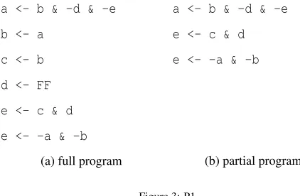
4.1. Comparison of C*- and Ł-interpretation
a <- b & -d & -e
b <- a
c <- b
d <- FF
e <- c & d
e <- -a & -b
(a) full program
a <- b & -d & -e
e <- c & d
e <- -a & -b
[image:29.612.188.399.267.405.2](b) partial program
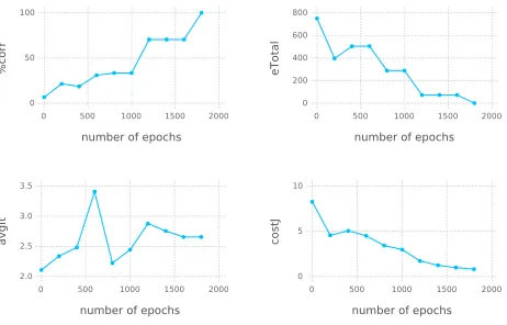
Figure 3: P1
The first example program illustrates that there are cases in which the method yields
good results under C*-interpretation. Training was done with learning rate and
mo-655
mentum of 0.05 under C*-interpretation and 0.02 under Ł-interpretation. During the
learning process a number of parameters are measured and reported for intermediate
results after every 200 training steps (500 in later examples). %corrindicates the
per-centage of correctly classified training samples, whileeTotalmeasures the total number
of errors, i.e. the number of incorrect rounded outputs over all output neurons and all
660
samples. In addition,avgItgives the average number of core iterations over all samples
andcostJis the total value of the error cost function. If the learning algorithm functions
correctly, one would expect a steady decline in the cost function, followed by decrease
of the total number of errors, which, in turn, leads to an overall rise in the amount
of correctly classified samples. Since%corr does not differentiate between samples
665
still high,%corrmay even increase, aseTotalis reduced, but more evenly distributed
across the samples. A similar distribution of errors may also happen in the relationship
between cost function and number of errors.
670
For the C- and C*-interpretation samples, training of the first test program tends to
converge after two to three thousand iterations. Depending on the random
initializa-tion, usually one of two optima is reached, the first one being at around 80% correct
classification, the second one at 100%.
number of epochs 0 500 1000 1500 2000 0
50 100
%corr
number of epochs 0 500 1000 1500 2000 0
200 400 600 800
eTotal
number of epochs 0 500 1000 1500 2000 2.0
2.5 3.0 3.5
avgIt
number of epochs
0 500 1000 1500 2000
0 5 10
[image:30.612.193.424.259.407.2]costJ
Figure 4: P1 training results under C*-interpretation
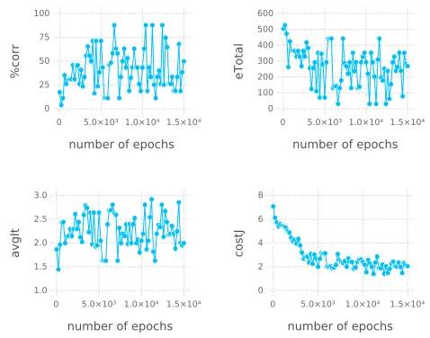
Under Łukasiewicz interpretation, the cost function can still be seen to generally
675
decrease, though not always monotonically, before it starts to fluctuate. Choosing
smaller learning rates remedies the fluctuation to some extent, but in many cases the
algorithm does not seem to converge even for small learning rates.10 The graphs also
show less correlation between the cost function and the total number of errors. This can
be attributed to the conflict resolution mechanism active under Ł-interpretation, which
680
may generate errors on the final output that are not accounted for in the cost function.
10Choosing very small learning rates (in the given example the threshold is at around 0.00003) leads to a
steady increase of the cost function. This has been observed across all examined cases but the source has not
number of epochs
0 5.0×10³ 1.0×10⁴ 1.5×10⁴
0 25 50 75 100 %corr
number of epochs
0 5.0×10³ 1.0×10⁴1.5×10⁴
0 100 200 300 400 500 600 eTotal
number of epochs
0 5.0×10³ 1.0×10⁴ 1.5×10⁴
1.0 1.5 2.0 2.5 3.0 avgIt
[image:31.612.188.427.129.317.2]number of epochs 0 5.0×10³ 1.0×10⁴ 1.5×10⁴ 0 2 4 6 8 costJ
Figure 5: P1 training results under Ł-interpretation
4.2. Correlation between error measures
Often times, as displayed by the second example, the learning process quickly gets
stuck in local optima under C*-interpretation. While the cost function converges, the
average number of iterations keeps fluctuating. Still, this does not seem to affect the
685
classification performance. Under Ł-interpretation, results are less clear-cut, but the
correlation betweencostJ,eTotaland%corris still clearly recognizable.
a <- b & c
b <- d & -e
c <- e
c <- b & -e
d <- a
e <- FF
(a) full program
a <- b & c
b <- d & -e
c <- e
c <- b & -e
(b) partial program
number of epochs
0 1×10³ 2×10³ 3×10³
0 20 40 60 80 %corr
number of epochs
0 1×10³ 2×10³ 3×10³ 0 200 400 600 800 eTotal
number of epochs 0 1×10³ 2×10³ 3×10³ 2.25 2.50 2.75 3.00 3.25 avgIt
[image:32.612.188.423.152.337.2]number of epochs 0 1×10³ 2×10³ 3×10³ 0 2 4 6 8 costJ
Figure 7: P2 training results under C*-interpretation
number of epochs
0 5.0×10³ 1.0×10 ⁴ 1.5×10 ⁴ 2.0×10 ⁴ 0 25 50 75 100 %corr
number of epochs
0 5.0×10³ 1.0×10 ⁴ 1.5×10 ⁴ 2.0×10 ⁴ 0 100 200 300 400 500 eTotal
number of epochs
0 5.0×10³ 1.0×10 ⁴ 1.5×10 ⁴ 2.0×10 ⁴ 1.5 2.0 2.5 3.0 3.5 avgIt
number of epochs
0 5.0×10³ 1.0×10 ⁴ 1.5×10 ⁴ 2.0×10 ⁴ 0 2 4 6 8 costJ
[image:32.612.191.421.426.614.2]4.3. The problem of hidden errors
The third program to be examined contains eight atoms, three more than the
pre-vious programs. This adds six neurons to the network and increases the number of
690
training samples from 243 to 6561. The fluctuation in the plots can in part be explained
by this fact. Steps of 500 samples make up less than 10% of the total sample size and
may at times lead the algorithm in different directions.
What is interesting about this example, is how the algorithm can be observed
plum-meting in overall performance in the first 500 training steps. This can be attributed to
695
two factors. Under the logistic cost function, which incentivises many smaller errors
over fewer large ones, distributing the error may serve to reduce the overall cost, but
increase the total amount. Secondly, the backpropagation algorithm is based on the
network output. And as the final output is created only after all facts from the
in-put, backpropagation will perceive all misclassifications which are fixed by this final
700
step. Correcting for these errors will decrease the cost function, but does not increase
the core’s performance. Under Ł-interpretation, the contradiction resolution step
con-tributes to this problem with an additional layer of error correction invisible to the
learning algorithm. Moreover, this step cannot be modeled without inhibitory
connec-tions, which leaves the algorithm trying—and failing—to correct an error that does
705
not actually exist. There may be multiple reasons for the weak performance under
Ł-interpretation, but this is certainly one of them.
In this example, these shortcomings are underlined by the fact that the initial
per-formance from partial background knowledge is much better than the local optimum
reached through training.
a <- TT
b <- a & -c
d <- c
d <- e
f <- e & -b
f <- a & g & -d
h <- FF
(a) full program
a <- TT
b <- a & -c
f <- e & -b
f <- a & g & -d
h <- FF
[image:34.612.186.417.115.504.2](b) partial program
Figure 9: P3
number of epochs
0 5.0×10³ 1.0×10 ⁴ 1.5×10 ⁴ 2.0×10 ⁴ 0 5 10 15 20 %corr
number of epochs
0 5.0×10³ 1.0×10 ⁴ 1.5×10 ⁴ 2.0×10 ⁴ 8.0×10³ 1.0×10⁴ 1.2×10⁴ 1.4×10⁴ 1.6×10⁴ eTotal
number of epochs
0 5.0×10³ 1.0×10 ⁴ 1.5×10 ⁴ 2.0×10 ⁴ 2.0 2.1 2.2 2.3 2.4 2.5 2.6 avgIt
number of epochs
0 5.0×10³ 1.0×10 ⁴ 1.5×10 ⁴ 2.0×10 ⁴ 0.0 2.5 5.0 7.5 10.0 costJ
number of epochs
0 5.0×10³ 1.0×10⁴
0 10 20 30 40
%corr
number of epochs
0 5.0×10³ 1.0×10⁴
0 5.0×10³
1.0×10⁴
1.5×10⁴
2.0×10⁴
eTotal
number of epochs
0 5.0×10³ 1.0×10⁴
1.8 2.0 2.2 2.4 2.6
avgIt
number of epochs
0 5.0×10³ 1.0×10⁴
0.0 2.5 5.0 7.5 10.0
[image:35.612.188.427.130.314.2]costJ
Figure 11: P3 training results under Ł-interpretation
4.4. Core compression
The final program examined here, is simply a long chain of inferences. The training
results are meant to highlight a phenomenon that is less pronounced but observable in
most trained cores. In this extreme case the partial program starts with an average
number of iterations of 4.14, which immediately drops to around 2, changing very
715
little thereafter. This number includes the last iteration where input and output must
be equal. Therefore, in all but very few cases, the inference is compressed into one
iteration. In general, trained cores tend to have fewer iterations on average than their
translated counterparts. This can be explained by the fact, that the backpropagation
algorithm does not take multiple iterations into account and optimizes for correct output
720
after just one iteration. This property does not decrease the performance of trained
b <- a
c <- b
d <- c
e <- d
f <- e
g <- f
g <- FF
(a) full program
b <- a
c <- b
d <- c
e <- d
f <- e
g <- FF
[image:36.612.185.426.116.504.2](b) partial program
Figure 12: P4
number of epochs
0 5.0×10³ 1.0×10⁴
0 10 20 30 40 50 60 %corr
number of epochs
0 5.0×10³ 1.0×10⁴
0 2.0×10³ 4.0×10³ 6.0×10³ 8.0×10³ eTotal
number of epochs
0 5.0×10³ 1.0×10⁴
1 2 3 4 5 avgIt
number of epochs
0 5.0×10³ 1.0×10⁴
5 6 7 8 9 10 costJ
Figure 13: P4 training results under C*-interpretation
4.5. Analysis through rule extraction
The developed rule extraction method is not yet suited to provide a complete picture
of the information contained in a core, but it may be used to take a look at individual
725
neurons and their activation rules. This can be done both for translated and trained
out(d>) a> a⊥ b> b⊥ c> c⊥ d> d⊥ e> e⊥ f> f⊥ g> g⊥ h> h⊥
translated 1 0 0 0 0 1 0 0 0 0 0 0 0 0 0 0 0
translated 2 0 0 0 0 0 0 1 0 0 0 0 0 0 0 0 0
translated 3 0 0 0 0 0 0 0 0 1 0 0 0 0 0 0 0
trained 1 0 0 0 0 1 0 0 0 0 0 0 0 0 0 0 0
trained 2 0 0 0 0 0 0 1 0 0 0 0 0 0 0 0 0
trained 3 0 0 0 0 0 0 0 0 1 0 0 0 0 0 0 0
Figure 14: Extracted minimal activating inputs ofd>in P3
out(f>) a> a⊥ b> b⊥ c> c⊥ d> d⊥ e> e⊥ f> f⊥ g> g⊥ h> h⊥
translated 1 0 0 0 0 0 0 0 0 0 0 1 0 0 0 0 0
translated 2 0 0 0 0 1 0 0 0 1 0 0 0 0 0 0 0
translated 3 0 0 0 0 0 1 0 0 0 1 0 0 1 0 0 0
trained 1 0 0 0 0 0 0 0 0 1 0 0 0 0 0 0 0
trained 2 0 0 0 0 0 0 0 0 0 0 1 0 0 0 0 0
Figure 15: Extracted minimal activating inputs off>in P3
In the third example above, for instance, in which the core was generated from the
program P3 with two missing clausesd <- candd <- eand then trained, it turns
out that thed>neuron’s activation rules in the trained core match the full program.
730
While learning was successful with regard tod>,d⊥does not show any activation in
the trained core, whereas the core containing the complete translated program has an
activation ind⊥when bothc⊥ande⊥are active.
These findings alone do not explain, why the trained core classifies less than 10%
of samples correctly. Looking further, it can be found that other inference structures
735
have largely broken down. For instance,f>has three activation rules in the core
con-taining the complete program. In the trained core, two rules are extracted, one of which
is wrong. This does not mean, that the connections to thef>output neuron are
neces-sarily wrong. Due to the core’s multiple iterations, the activation patterns of different
![Figure 1: A conceptual overview of the neural-symbolic cycle (as introduced in [11]).](https://thumb-us.123doks.com/thumbv2/123dok_us/1376033.90867/4.612.145.468.137.238/figure-conceptual-overview-neural-symbolic-cycle-introduced.webp)