Multivariate Asset Models Using Levy Processes and Applications

City, University of London Institutional Repository

Citation

:

10.1080/1351847X.2013.870917

This is the accepted version of the paper.

This version of the publication may differ from the final published

version.

Permanent repository link:

Link to published version

:

Copyright and reuse:

City Research Online aims to make research

outputs of City, University of London available to a wider audience.

Copyright and Moral Rights remain with the author(s) and/or copyright

holders. URLs from City Research Online may be freely distributed and

linked to.

City Research Online: http://openaccess.city.ac.uk/ [email protected]

Laura Ballotta∗ Efrem Bonfiglioli†

November 2013

Abstract

In this paper we propose a multivariate asset model based on L´evy processes for pricing of products written on more than one underlying asset. Our construction is based on a two factor representation of the dynamics of the asset log-returns. We investigate the properties of the model and introduce a multivariate generalization of some processes which are quite common in financial applications, such as subordinated Brownian motions, jump diffusion processes and time changed L´evy processes. Finally, we explore the issue of model calibration for the proposed setting and illustrate its robustness on a number of numerical examples.

Keywords: Jump Diffusion process, L´evy processes, model calibration, multinames derivative contracts, subordinated Brownian motions, time changed L´evy processes.

JEL Classification: G13, G12, C63, D52

1

Introduction

The aim of this paper is to introduce a simple, parsimonious and robust model for multivari-ate L´evy processes with dependence between components, which can be easily implemented for financial applications, such as the pricing of several types of multi-names derivative contracts commonly used for example in the credit and the energy markets. The interest in the construc-tion of multidimensional asset models based on L´evy processes is motivated by the importance of capturing market shocks using more refined distribution assumptions compared to the standard Gaussian framework, as highlighted by the recent crisis in the financial markets.

The proposed approach is based on a parsimonious two-factor linear representation of the assets (log)-returns, in the sense that it uses a linear combination of two independent L´evy pro-cesses representing respectively the systematic factor and the idiosyncratic shock. Hence, the model has a simple and intuitive economic interpretation and retains a high degree of mathe-matical tractability, as the multivariate characteristic function is always available in closed form.

∗

Faculty of Finance, Cass Business School; Email: [email protected]

†

Itau-Unibanco; Email: [email protected]

Further, dependence is generated by the chosen construction and the features of the distribu-tion of the processes chosen as systematic and idiosyncratic components. Our construcdistribu-tion can be further applied to originate multidimensional versions of time changed L´evy processes with dependence between components. This would allow to incorporate stochastic volatility features which are shown to improve the performance of L´evy processes in pricing options across different maturities (see Carr et al., 2003; Carr and Wu, 2004; Huang and Wu, 2004, for example).

The idea of inducing correlation via a factor approach dates back to Vasicek (1987) for the case of Brownian motions; the application of linear transformations has been extensively adopted in the literature for the case of L´evy processes as well. We cite, amongst others, the approaches put forward by Baxter (2007), Moosbrucker (2006a,b), Lindskog and McNeil (2003), Brigo et al. (2007), Semeraro (2008) and Luciano and Semeraro (2010). In more details, Baxter (2007) and Moosbrucker (2006a,b) use a factor copula approach for both subordinated Brownian motions and Jump Diffusion (JD) processes, whilst Lindskog and McNeil (2003) make use of linear combinations to develop a common Poisson shock process framework for dependent events frequencies in the context of insurance loss modelling and credit risk modelling. This approach is then extended in Brigo et al. (2007) to a formulation which avoids repeated defaults at both cluster level and single name level. Semeraro (2008) and Luciano and Semeraro (2010) instead apply the factor approach to build multivariate subordinators from which they derive the multivariate version of several families of subordinated Brownian motions, such as the Variance Gamma process, in this way generalizing the approaches of Luciano and Schoutens (2006), Cont and Tankov (2004), Leoni and Schoutens (2006) and Eberlein and Madan (2009).

In spite of being in general simple and relatively parsimonious, these approaches present a number of drawbacks, including restrictions on the range of possible dependencies and the set of attainable values for the correlation coefficient. This is also documented, for example, by Wallmeir and Diethelm (2012) whose empirical analysis shows the limited potential to match ob-served correlations of the multivariate Variance Gamma models of Leoni and Schoutens (2006) and Semeraro (2008). We note that for the case of subordinated Brownian motions, Semer-aro (2008) and Luciano and SemerSemer-aro (2010) improve the richness of the correlation struc-ture through an alternative construction which uses correlated Brownian motions. However, as pointed out by the the same authors, this is achieved at the cost of increasing the number of pa-rameters required for calibration: the presence of a correlation matrix for the Brownian motion part of the components, in fact, implies that the number of parameters grows with the square of the number of assets included in the basket, whilst market data available for calibration is usually linear in the number of instruments.

to jump diffusion processes. In particular, in the case of jump diffusion processes, it allows the distribution of the jump sizes to depend on the nature of the underlying shock; in the case of subordinated Brownian motions, instead, the construction does not necessarily rely on the process chosen as subordinator. This is of relevance, for example, in those cases in which the simulation of the process subordinator proves inefficient, as in the case of the CGMY process (see Ballotta and Kyriacou, 2014, for example). Further, our model is flexible enough to accommodate complete dependence, independence, positive and negative linear correlation, and is relatively parsimonious in terms of the overall number of parameters involved, as this grows linearly with the number of assets, which facilitates its calibration to market data.

Finally, we note that model calibration to market data is an essential step for practical pricing applications; however, calibration of any multivariate model requires the existence of actively traded multi-names derivatives, and this is not the case in general. Hence, in the paper we explore the implications of this issue on the proposed construction and the potential limitations. The remaining of the paper is organized as follows. In section 2, we introduce our class of multivariate L´evy processes, investigate its general properties and apply it to build multivariate subordinated Brownian motions and jump diffusion processes. A financial application focussed on model calibration and testing the robustness and the flexibility of the model is presented in section 3; in this section, we also consider the pricing of spread options in view of recovering information on the implied correlation matrix. Extensions to the case of time changed L´evy processes are introduced in section 4; section 5 concludes.

2

Multivariate L´

evy process via linear transformation

L´evy processes are characterized by independent and stationary increments; they are fully de-scribed by their characteristic function which admits L´evy-Khintchine representation

φ(u;t) = etϕ(u), u∈_R

ϕ(u) = iuα−u2σ 2

2 +

Z

R

eiux−1−iux1(|x|<1)

Π (dx).

The terms in the characteristic exponent, ϕ(·), i.e. (α, σ,Π) represent the characteristic triple of the L´evy process. The parameter α∈ _Rdescribes the drift of the process, σ >0 represents its diffusion part, whilst the jumps are fully characterized by the L´evy measure Π, i.e. a positive measure satisfyingR

R

2.1 General framework

To construct a multivariate L´evy process with dependent components, we use the property that these processes are invariant under linear transformations. The main result is given in the following.

Proposition 1 LetZ(t),Yj(t),j= 1, ..., nbe independent L´evy processes on a probability space

(Ω,F,P), with characteristic functionsφZ(u;t)andφYj(u;t), forj = 1, ..., nrespectively. Then,

for aj ∈R, j= 1, ..., n

X(t) = (X1(t), ...Xn(t))> = (Y1(t) +a1Z(t), ..., Yn(t) +anZ(t))>

is a L´evy process on Rn. The resulting characteristic function is

φX(u;t) =φZ





n

X

j=1 ajuj;t





n

Y

j=1

φYj(uj;t), u∈R

n_{. (1)}

Corollary 2 Let X(t) be the multivariate L´evy process introduced in Proposition 1. Then.

(i) For j= 1, ..., n, the mth cumulant,cm, of the jth component of X(t) is

cm(Xj(t)) =t

cm(Yj(1)) +amj cm(Z(1))

. (2)

(ii) For any j6=l, the covariance between the jth and lth components ofX(t) is

Cov(Xj(t), Xl(t)) =ajalVar(Z(1))t.

The proof of both Proposition 1 and Corollary 2 follows from the properties of L´evy processes (see, for example Cont and Tankov, 2004, Theorem 4.1).

The construction given in Proposition 1 offers a simple and intuitive economic interpretation as for each margin,Xj, the processZcan be considered as the systematic part of the risk, whilst

the process Yj can be seen as capturing the idiosyncratic shock. Due to the presence of the

Corollary 3 For each t≥0, X(t) is positive associated, i.e.

Cov(f(X(t)), g(X(t)))≥0

for all non decreasing function f, g :Rn →R for which the covariance is well-defined, if either aj ≥0 for j= 1, ..., n or aj ≤0 for j= 1, ..., n.

In the more general case in which the coefficientsaj do not have the same sign for j = 1, ..., n,

the components Xj(t) and Xl(t), j 6= l, are pairwise negative quadrant dependent if ajal <0.

Moreover, it follows directly from the construction ofX(t) that the components are condition-ally independent; further, ifY(t) is degenerate, the components of X(t) are perfectly (linear) dependent; on the other hand, if Z(t) is degenerate, the components of X(t) are independent.

For the case of the proposed construction, the dependence between components of the mul-tivariate L´evy processX(t) is correctly described by the pairwise linear correlation coefficient

ρX_jl =Corr(Xj(t), Xl(t)) =

ajalVar(Z(1)) p

Var(Xj(1))

p

Var(Xl(1))

, (3)

(see Embrechts et al., 2002, for example). Indeed, ρX_jl = 0 if and only if either ajal = 0 or

Var(Z(1)) = 0, i.e. Z is degenerate and the margins are independent. Moreover, |ρXjl| = 1

if and only if Y(t) is degenerate and there is no idiosyncratic factor in the margins. Further,

signρX_jl=sign(ajal) and therefore both positive and negative correlation can be

accommo-dated. Finally, for fixed aj = ¯a > 0 (resp. aj = ¯a < 0), ρX_jl is a monotone increasing (resp.

decreasing) function of al, which can take any value from −1 to 1 (resp. from 1 to -1). In

particular,ρX_jl = 0 if either ¯a= 0, oral= 0 or both, whilst |ρXjl|= 1 as a limit case for ¯a→ ∞

and al→ ∞.

The previous results highlight an advantage of our model compared to the multivariate sub-ordinator approach of Semeraro (2008) and Luciano and Semeraro (2010), and the factor copula approach of Baxter (2007) and Moosbrucker (2006a,b). All these constructions, in fact, can only accommodate strictly positive correlation values due to restrictions on the parameter control-ling the correlation coefficient, which are required to ensure the existence of the characteristic function of the processes involved. Moreover in the case of Semeraro (2008) and Luciano and Semeraro (2010), the correlation coefficient can be zero (for symmetric subordinated Brownian motions) even though the processes are still dependent.

Finally, the pairwise linear correlation between the margin processes can be expressed in terms of the correlation between each margin and the systematic component as

Corr(Xj(t), Z(t)) =aj

s

Var(Z(1))

Var(Xj(1))

implying thatρX_jl =Corr(Xj(t), Z(t))Corr(Xl(t), Z(t)).

The multidimensional modelling approach put forward in this section is quite flexible as it allows to specify any univariate L´evy process for Y(t) and Z(t); the resulting distribution of the margin might not be known analytically, but it is still accessible via the corresponding characteristic function. On the other hand, for any chosen distribution for the margin process

X(t), it is possible to impose convolution conditions on the processes Y(t) and Z(t) so that the linear combination Y(t) +aZ(t) has the same given distribution of X(t). This could be particularly convenient in the case in which the multivariate L´evy processX(t) is used to build a model for financial assets which is consistent with the information provided by traded vanilla (univariate) options. As in general correlation cannot be directly observed in the market due to lack of sufficiently liquid multinames derivative contracts (and therefore reliable quotes for these instruments), by imposing convolution the calibration of the marginal distribution to observable market data would be independent of the fitting of the correlation matrix, and therefore the parameters governing the idiosyncratic and the systematic processes. These parameters would be recovered at a second stage from any given correlation matrix and the relevant restrictions imposed by the convolution. In more details, to facilitate the convolution, we chooseX(t),Y(t) and Z(t) from the same family of processes and, given the margins parameters, we solve

ϕXj(u) =ϕY j(u) +ϕZ(aju) j= 1,2, ..., n. (5)

This implies that, if m is the number of parameters describing the processes Xj(t), Yj(t) and

Z(t), and the parameters of the margin processes are given, for a known correlation matrix the fitting of the joint distribution requires n(m+ 1) +m parameters. As shown by eq. (3), we can recover the m parameters describing the common process Z(t) and the n loadings aj,

j= 1,2, ..., n, through the correlation matrix subject to relevant convolution conditions arising from eq. (5). Thenm parameters of the idiosyncratic process Yj(t) would then be obtained by

solving eq. (5) directly.

We note the following. In first place, the presence of convolution conditions on the parameters of the idiosyncratic and systematic processes does not restrict the behaviour of the correlation coefficient (3), as their effect would be to ensure that the cumulantscm(Xj(t)) and cm(Yj(t) +

ajZ(t)) match for j = 1, ..., n. Further, convolution conditions would not be necessary for

applications in which keeping the number of parameters small when dealing with univariate contracts is not of particular relevance, and reliable information on the correlation matrix is available.

2.2 Multivariate subordinated Brownian motions

A subordinated Brownian motion X = (X(t) :t≥0) is a L´evy process obtained by observing a (arithmetic) Brownian motion on a time scale governed by an independent subordinator, i.e. an increasing, positive L´evy process. HenceX(t) has general form

X(t) =θG(t) +σW (G(t)), θ∈R, σ >0, (6)

where W = (W(t) :t≥0) is a Brownian motion and G = (G(t) :t≥0) is a subordinator independent ofW. The resulting characteristic function is

φX(u;t) =e tϕG

uθ+iu2σ2

2

, u∈_R, (7)

whereϕG(·) denotes the characteristic exponent of the subordinator.

Constructing L´evy processes by subordination has particular economic appeal as, in first place, empirical evidence shows that stock log-returns are Gaussian but only under trade time, rather than standard calendar time (see Geman and An´e, 1996, for example). Further, the time change construction recognizes that stock prices are largely driven by news, and the time between one piece of news and the next is random as is its impact.

In general, the parameters of the distribution of the subordinator are chosen so thatEG(t) = t, in order to guarantee that the stochastic clock G(t) is an unbiased reflection of calendar time (see Madan et al., 1998, for example). The law of the increments of G(t) allows us to characterize the resulting process. There are different methods for choosing a subordinator which is suitable for financial modelling; one class of such processes which proves to be quite popular due to its mathematical tractability is the family of tempered stable subordinators, which have characteristic exponent

ϕG(u) =

α−1

αk

1− iuk

1−α α

−1

, u∈R, (8)

wherek >0 is the variance rate of G(t) andα ∈[0,1) is the index of stability. In particular, if

α= 0, expression (8) is to be understood in a limiting sense andG(t) is a Gamma process so that

X(t) is a (asymmetric) VG process (see Madan et al., 1998, for example). If, instead, α= 1/2, the subordinator follows an Inverse Gaussian process and X(t) is the NIG process introduced by Barndorff-Nielsen (1995). We note that the probability density of tempered stable processes is known in explicit form only for these values of the stability index (i.e. α = 0 and α = 1/2), however, through eq. (7) - (8) it is possible to construct subordinated Brownian motions for any value of α∈[0,1).

follow Proposition 1 and let Yj(t) and Z(t) be independent subordinated Brownian motions

chosen from the same family of distributions, and obtained by subordinating respectively a Brownian motion with drift βj ∈ R and volatility γj > 0 by an unbiased subordinator GY j,

and a Brownian motion with drift βZ ∈R and volatility γZ > 0 by an unbiased subordinator

GZ. Then, X(t) is a multivariate subordinated Brownian motion with margins of the same

distribution’s class asYj(t) andZ(t) if the convolution condition (5) is satisfied.

For sake of illustration, in the following we consider the case in which the subordinatorsGj,

GY j, for j= 1, ..., nand GZ are unbiased tempered stable processes with variance rates kj >0,

νj >0 and νZ >0 respectively. Then, eq. (5) and (8) imply

(

kjθj =νZajβZ j = 1, ..., n

kjσj2=νZa2jγZ2 j= 1, ..., n

(9)

consequently

θj =βj+ajβZ, σj2=γj2+a2jγZ2, kj =νjνZ/(νj+νZ)

(10)

The subordinators, in fact, are assumed to have the same stability indexαin order to guarantee thatXj(t),Yj(t) and Z(t) belong to the same family of distributions.

We note the following. Firstly, the application of Proposition 1 only requires knowledge of the characteristic function of the subordinated Brownian motions, whilst the exact features of the subordinator processes are not necessary (see, for example Ballotta and Kyriacou, 2014, for the construction based on Proposition 1 of a multivariate CGMY process, which is a subordinated Brownian motion whose subordinator’s distribution is not available in explicit form). Secondly, in this construction dependence stems from both the subordinator and the associated Wiener process. In particular, somehow similar to the model of Luciano and Semeraro (2010), our approach allows for the activity of the (margin) stochastic clock to be governed by a systematic component and a component which is instead asset specific, as supported by the empirical analysis performed by Lo and Wang (2000).

Example 1 (The VG process) LetG(t) be a gamma process, i.e. a tempered stable process with scale parameter α= 0; thenX(t) is a VG process with characteristic function

φX(u;t) =

1−iuθk+u2σ 2

2 k

−_kt

, u∈_R.

parameters (θj, σj, kj) constructed as described above and characteristic function

φX(u;t) =



1−iβZνZ n

X

j=1

ajuj+

γ_Z2

2 νZ





n

X

j=1 ajuj

  2  − t νZ _n Y j=1

1−iujβjνj +u2j

γ_j2

2 νj

!−t

νj

.

The coefficient of pairwise correlation given by equation (3) in this case reads

ρX_jl = ajal γ

2

Z+βZ2νZ

q σ2

j +θj2kj

q σ2

l +θ2lkl

. (11)

Example 2 (The NIG process) In the case in which the tempered stable subordinatorG(t) has scale parameter α = 1/2, i.e. is an Inverse Gaussian process, then X(t) is a NIG process with characteristic function

φX(u;t) =e

t k(1−

√

1−2iuθk+u2_σ2_k)

, u∈_R.

Under the convolution restrictions (9), the margins Xj(t) are NIG processes with parameters

(θj, σj, kj) as constructed above. The resulting characteristic function of the multivariate NIG

process is

φX(u;t) = etϕ(u)

ϕ(u) = 1

νZ



 1−

v u u u

t1−2iβZνZ

n

X

j=1

ajuj+γ_Z2νZ





n

X

j=1 ajuj

  2   + n X j=1 1 νj

1−q1−2iujβjνj +u2jγj2νj

.

Equation (11) describes the pairwise correlation coefficient also in this case.

As both the VG and NIG are 3-parameter processes, the number of parameters required for the joint fit, given the margins, is (4n+ 3), of which 3 +n are observed from the correlation matrix subject to conditions (9), and 3nare obtained from the conditions on drift and diffusion coefficients.

2.3 Multivariate jump-diffusion (JD) process

they experience large jumps upon the arrival of important information with more than just a marginal impact. By its very nature, important information arrives only at discrete points in time and the jumps it causes have finite activity. A motion portraying such a dynamic is a jump-diffusion process, which can be decomposed as the sum of a Brownian motion with drift and an independent compound Poisson process. Hence, a L´evy process in the JD class has form

X(t) =µt+σW(t) +

N(t)

X

k=1

ξ(k), µ∈_R, σ >0,

whereW = (W (t) :t≥0) is a Brownian motion,N = (N(t) :t≥0) is a Poisson process count-ing the jumps of X and ξ(k) are i.i.d. random variables capturing the jump sizes (severities).

W,N and ξ are independent of each other.

We assume that the rate of arrival of the Poisson process isλ >0. In this case, we say that the process X(t) has parameters (µ, σ, λ) and jump sizes distributed as a random variable ξ; the resulting characteristic function is

φX(u;t) = e t

iuµ−u2σ₂2+λ(φξ(u)−1)

,

φξ(u) = E

eiuξ, u∈_R.

Popular examples of JD processes used in finance are the so-called Merton process (Merton, 1976), for which the jump sizes are Gaussian, and the Kou process (Kou, 2002) in which case the jump sizes follow an asymmetric double exponential distribution.

In order to construct the multivariate version of the JD process, we follow the same steps as in the previous sections and let the idiosyncratic factor,Yj, and the global factor,Z, to be two

independent JD processes, respectively with parameters (βj, γj, δj) and jump sizes distributed

as a random variable ηj, and (βZ, γZ, δZ) and jump sizes distributed as a random variableηZ.

The corresponding pairwise correlation coefficient is

ρX_jl = ajal γ

2

Z+δZE ηZ2

r σ2

j +λjE

ξ2

j

q σ2

l +λlE ξl2

. (12)

Further, for the convolution condition (5) to hold, i.e. for the process X(t) =Y(t) +aZ(t) to be a multivariate JD process, whose margins have parameters (µj, σj, λj) and jump sizes

distributed as a random variable ξj, we require

µj =βj+ajβZ, σj2 =γj2+a2jγZ2

further, as the Poisson process is closed under convolution, we also impose

λj =δj +δZ, (14)

from which it follows that eq. (5) reduces to the following convolution on the distribution of the jump sizes:

φξj(u) =

δjφηj(u) +δZφηZ(aju)

δj+δZ

, u∈_R. (15)

We note the following. Firstly, under the proposed construction, the compound Poisson process components are allowed to jump at different points in time. Secondly, the convolution conditions reported above show the decomposition of both the continuous part of the risk and the pure jump one into their corresponding asset specific part and the one common to the entire basket under consideration. Further, the proposed construction of multivariate JD processes falls in the more general common Poisson shock framework, reviewed in Lindskog and McNeil (2003) and further extended by Brigo et al. (2007). In our case, we use only two different types of shock (systematic and idiosyncratic); however, the distribution of the jump sizes depends on the nature of the underlying shock.

We note that a simple solution to eq. (15) can be obtained by assuming thatξj, ηj and ajηZ

are identically distributed. This is the case discussed by Moosbrucker (2006a) . However, in the following we do not consider this alternative as it imposes the unrealistic restriction that the jump sizes of each margin and the ones of its idiosyncratic component are identically distributed. Therefore, we make use of the (numerical) solution of eq. (15). In particular, as this condition indicates that the margins’ jump size distribution is given by a mixture of the distributions of the components’ jump sizes, we solve the resulting missing data problem by moment matching.

Example 3 (The Merton process) Assume that the distribution of the jump sizes is Gaus-sian. Then, ifηj ∼N

ϑY j, υ2Y j

andηZ∼N ϑZ, υ2Z

, the processXj(t) =Yj(t) +ajZ(t) is a

Merton JD process with parameters (µj, σj, λj) as defined above, and jump sizesξj ∼N

ϑj, υ_j2

, whereϑj and υj are the solutions of

eiuϑj−u2 υ_j2

2 = δje

iuϑY j−u2 υ2

Y j

2 +δ_ZeiuajϑZ−u 2a

2

j υ2Z

2

δj+δZ

, u∈R. (16)

The above implies

ϑj =

δjϑY j+δZajϑZ

δj+δZ

,

υ_j2 = δj(ϑ

2

Y j+υ2Y j) +δZaj2(ϑ2Z+υZ2)

δj+δZ

The coefficient of correlation is given by equation (12), with

E ξj2

= ϑ2_j +υ_j2, ∀j= 1, ..., n

E ηZ2

= ϑ2_Z+υ_Z2.

Example 4 (The Kou process) In the case of the Kou process, the jump sizes follow a double exponential distribution with parameters (p, α+, α−), i.e. their density function is given by

pα+e−α+y1(y≥0)+ (1−p)α−eα

−_y

1(y<0), α+, α−∈R++, p∈[0,1].

Thus, ifηj,ηZ,ξjhave a double exponential distribution respectively with parameters (pY j, α+Y j, α

−

Y j),

(pZ, α+_Z, α−_Z), (pj, α_j+, α−_j ), then, for the convolution condition (15) to hold, these parameters

must satisfy the following

pj

α+_j

α+_j −iu+ (1−pj) α−_j

α−_j +iu =

1

δj+δZ

" pY j

δjα+Y j

α+_{Y j}−iu + (1−pY j)

δjα−Y j

α−_{Y j}+iu+pZ

δZα+_Z

α+_Z −iaju

+ (1−pZ)

δZα−_Z

α−_Z +iaju

# .(17)

The correlation coefficient is obtained from equation (12) for

E ξj2

= 2



 

pj

α+_j 2

+ 1−pj

α−_j2





, ∀j= 1, ..., n

E η2Z

= 2 pZ

α+_Z2

+1−pZ

α−_Z2 !

.

Finally, we note that for the multivariate Kou model, the reconstruction of the margin param-eters (p, α+, α−) from the components parameters can only be performed numerically.

In the following, we consider applications of our multivariate approach to option pricing problems; therefore, without loss of generality, we consider the case of a JD process with no drift, i.e. we setµj =βj =βZ = 0 for j= 1, ..., n. This implies that for the joint fit, given the

3

Multivariate asset modelling: calibration and derivative

pric-ing

In this section we analyze the calibration of the multivariate L´evy process model to market data in view of applications to the problem of pricing multi-assets products.

To this purpose, we consider a frictionless market in which (equity) asset log-returns are modelled by the multivariate L´evy process defined in Proposition 1, so that under any risk neutral martingale measure asset prices are given by

Sj(t) =Sj(0)e(r−qj−ϕXj(−i))t+Xj(t), j= 1, ..., n

where r > 0 is the risk free rate of interest, Sj(0) and qj denote respectively the spot price

and the dividend yield of the jth _{asset, and ϕ}

Xj(−i) is the exponential compensator of the jth

component of the multivariate L´evy process,Xj(t). As in general the given market is incomplete,

there are infinitely many risk neutral martingale measures; the availability of market prices for European vanilla options, though, allows us to “complete” the market and extract the pricing measure by calibration.

As outlined in the previous sections, the full calibration procedure should use both single-name and multi-single-names derivatives in order to access information on the log-returns correlation matrix as well. However, in general suitable multi-names contracts are not sufficiently liquid to generate reliable estimates. Therefore, we assume that option traders views about this cor-relation is strongly based on observed asset prices; we further explore a procedure with which information about the market consensus on correlation could be recovered, in a way similar to the one used to extract implied volatility from vanilla options, if a suitable number of prices of exotic options (that are sensitive to correlation) is available. Finally, we note that the cal-ibration of the model can only be solved numerically via constrained least square; hence, we analyze the resulting approximation error by quantifying the difference between the moments of the distribution of the processesX(t), calculated using the components parameters in conjunc-tion with eq. (2), and the same moments calculated instead using the margin parameters and the corresponding model exact formulae (reported in B for the case of subordinated Brownian motions and C for the case of JD processes).

3.1 Model calibration: a 3-asset case

We test the flexibility of the model by calibrating it to option prices on Ford Motor Company, Abbott Laboratories and Baxter International Inc. We use Bloomberg quotes at three different valuation dates, September 30, 2008, February 27, 2009 and September 30, 2009, in order to explore the behaviour of the proposed model when fitting different correlation values. A synopsis of the three assets is reported in Table 1. The risk free rate of interest is taken from Bloomberg as well in correspondence of the relevant dates. Correlation between assets log-returns has been estimated on a time window of 125 days up to (and including) the valuation date.

The three assets considered in this analysis are constituents of the S&P100 index, and rep-resent three different industries: automotive, drug manufacturers and medical instruments and supplies respectively. Abbott Laboratories and Baxter International Inc. are part of the same healthcare sector. Further, from Table 1 we observe that in September 2008 the three assets exhibit positive correlation, at a level which is fairly similar between Ford and the remaining two assets, whilst it is significantly higher between Abbott and Baxter. This date, in fact, co-incides with the peak of the financial crisis which led to the collapse of Lehman Brothers; the car industry was also experiencing a particularly difficult period following the General Motors liquidity crisis and the sales fall also reported by its main competitors. Correlation values fur-ther increase in February 2009, when the effects of the credit crisis are fully captured by the estimation procedure used in this analysis. These observations lead us to expect the common component Z(t) to play a significant role in the prices of Abbott Lab. and Baxter, whilst we expect it to have a smaller impact on Ford prices. The same consideration holds especially for the September 2009 valuation date, when Ford exhibits negative correlation with the other two assets considered in this analysis.

the relevant convolution conditions.

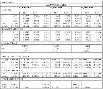
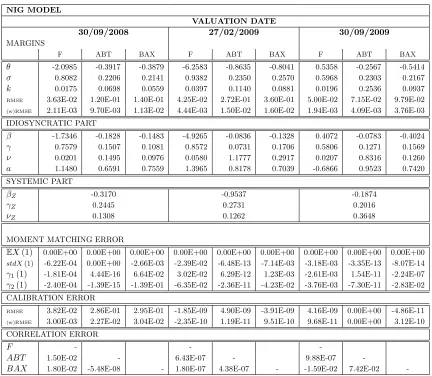
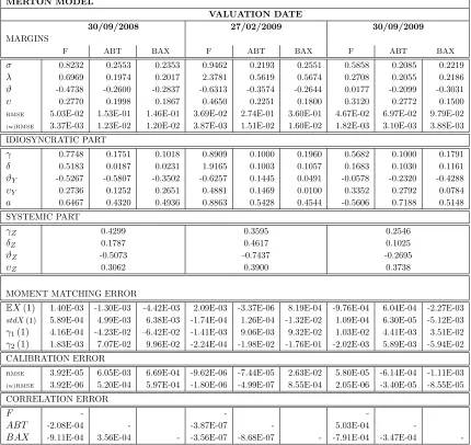
The calibrated parameters of the margins, the idiosyncratic components and the systematic process are reported in Tables 2-5 for all the valuation dates considered and models analysed in this paper. The Tables also report the accuracy with which the postulated linear combination reproduces the margin process distribution (which we quantify under the heading “Moment Matching Error”), and the error originated in fitting the given correlation matrix (heading “Correlation Error”). Further, Figures 1-2 show the QQ plots of the (simulated) samples of the margin process obtained by direct calibration to European vanilla options and the same process obtained, instead, by linear combination of the idiosyncratic process and the systematic process. In particular, in these plots we consider the case of the multivariate VG model and Merton JD model (similar results have been obtained for the other models presented in this paper and are available from the authors). These results illustrate the goodness of the convolution provided by the fitting procedure, although the accuracy of the approximation tends to deteriorate at the very far end of the tails. Also, the full range of observed correlations is captured with a satisfactory degree of accuracy.

As a further test, we re-calculate the prices of the European vanilla options using the joint characteristic function and quantify the error against the corresponding market data, as reported in Tables 2-5. The (weighted) root mean squared errors are very close to the ones generated by direct calibration of the marginal distribution, which shows that any potential approximation error introduced by the joint fitting procedure is relatively negligible for this type of application. We note though that the higher the number of parameters in the joint distribution, the less flexible the fitting of the multivariate model, which highlights the importance of having a parsi-monious margin model for the fitting procedure to converge efficiently. Finally, Figure 3 shows the volatilities recovered by the standard Black-Scholes formula in the case in which the input prices are generated by the multidimensional VG process. The plot also reports the original bid-ask volatilities obtained from market data.

of the total variance of Ford log-returns in September 2008, against 60% of the total variance of Abbot Lab. and 67% of Baxter. This changes in February 2009 to 14% for Ford, 90% for Abbott Lab. and 62% for Baxter. In September 2009, the contribution ofZ accounts for 10% of the total variation of Ford, and 49%-41% for Abbott Lab. and Baxter respectively. Similar considerations hold for the other models analyzed in this paper.

3.2 Pricing of Exotics and implied correlation

In this section, we consider the pricing of European style multi-names products in the market model calibrated in section 3.1. In particular, we consider the case of a spread (call) option with payoff at maturityT

(S1(T)−S2(T)−K)+.

The choice of this contract class is motivated by the fact that they carry information about the market consensus on correlation between the underlying assets.

In this example, we assume a joint VG dynamics for the log-returns of the two assets, with parameters obtained by the joint model calibration reported in Table 2. Further, we assume that the assets considered are Baxter and Abbott Lab. forj= 1,2 respectively; finally the valuation date is 27/02/2009. All prices are computed using the Fourier inversion method proposed by Hurd and Zhou (2009).

The “implied” correlation is obtained from the standard model using as input the spread option prices obtained under the multivariate VG model, and the implied volatility of each asset extracted from vanilla option prices computed under the VG model in correspondence of each strike and maturity. The results are presented in Figure 4 - panel (a). We note, in particular, that the implied correlation is higher than the historical correlation (which is fixed at 83% - see Table 1) in the case of in-the-money options (i.e. if K < A(0), for A(0) = S1(0)−S2(0)) and

it decreases as the option moves out-of-the-money and deep out-of-the-money (i.e. K > A(0)). This observed “skew” pattern is consistent with the so-called correlation leverage effect reported for example by Da Fonseca et al. (2007).

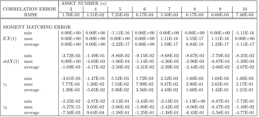
3.3 Model calibration in higher dimensions

We conclude this section with some additional comments on the performance of the model and the proposed 2-step calibration procedure when more than three assets are considered.

for the 5-assets and 10-assets cases are presented in Figures 5-6. We note that, as somewhat expected, the dimensionality of the problem affects both the quality of the correlation fit and the robustness of the numerical solution to the convolution conditions, especially as far as the tails of the distributions are concerned.

4

Extensions to multivariate time changed L´

evy processes: a

simple setting.

The multivariate L´evy process introduced in Proposition 1 can also be used as the basis for mul-tivariate time changed L´evy processes constructions, allowing for the introduction of stochastic volatility features. As L´evy processes have independent and stationary increments, in fact, they suffer in terms of fitting performance especially over medium-long maturities. In this respect, time changed L´evy processes represent a way to simultaneously and parsimoniously capture the fact that not only asset prices jump, but also returns volatilities are stochastic and are correlated to asset returns. These processes have been studied in the context of option pricing by, amongst others, Carr et al. (2003), Carr and Wu (2004), and Huang and Wu (2004) (see Appendix B).

For a simple construction, let V(t) be a n-dimensional absolutely continuous time change with components of the form

Vj(t) = bjV(t)

= bj

Z t

0

v(s)ds j= 1, ..., n,

for positive constants bj, j = 1, ..., n, and a positive integrable process v(t) representing the

instantaneous (common) business activity rate. A multivariate time changed L´evy processB(t) can be then obtained by evaluating each component of a n-dimensional L´evy process X(t) as given in Proposition 1 on a time scale governed by V(t) so that

Bj(t) =Xj(Vj(t)) j = 1, ..., n.

The corresponding characteristic function of the margin process is given by

φBj(uj;t) =E h

E

eiujXj(Vj(t))

Vj(t)

i

uj ∈R, j= 1, ..., n; (18)

ifVj(t) is independent of Xj(t) for j= 1, ..., n, (18) reduces to

φBj(uj;t) =φV (−ibjϕXj(uj);t) j= 1, ..., n. (19)

are correlated (to capture the so called leverage effect) can be obtained using the leverage-neutral measure of Carr and Wu (2004). The corresponding multivariate characteristic function is therefore

φB(u;t) = φV (−ig(u;a,b) ;t) (20)

g(u;a,b) =

n

X

j=1

bjϕY j(uj)

+b₍₁₎ϕZ





(n)

X

l=(1) ulal



+

(n)

X

l=(2)

(bl−bl−1)ϕZ





(n)

X

k=(l) ukak



 (21)

where b_(j) is the j-th element of the sequence (b₍₁₎, b₍₂₎, ..., b_(n)) obtained by rearranging in increasing order the sequence of parameters (b1, b2, ..., bn) (and (1),(2), ...,(n) is a permutation

of 1,2, ..., n). Further, for anyj 6=l, the covariance between thejthand lth components ofB(t) is

Cov(Bj(t), Bl(t)) =ajalmin(bj, bl)E(V(t))Var(Z(1)) +bjblE(Xj(1))E(Xl(1))Var(V(t)), (22)

from which the correlation coefficient follows (the proof of equations (20)-(22) is provided in Appendix B.2). We note the limited dependence structure offered by the proposed construction due to the common time change applied to the base L´evy process; a full, richer construction of multivariate time changed L´evy processes is left to future research.

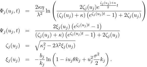
For an illustration, we consider the case of a multivariate VG process (as given in section 2.2) time changed by an independent integrated CIR process (as in Carr et al. (2003)), so that

dv(t) =κ(η−v(t))dt+λpv(t)dW¯(t),

where ¯W(t) is a standard Brownian motion independent of the base processX(t). The charac-teristic function of V(t) is well known from standard results on affine processes (see Filipovi´c, 2009, for example); therefore (19) reads

with

Φj(uj, t) =

2κη λ2 ln





2ζj(uj)e

ζj(_uj)+κ

2 t

(ζj(uj) +κ) eζj(uj)t−1

+ 2ζj(uj)





Ψj(uj, t) =

2ξj(uj) eζj(uj)t−1

(ζj(uj) +κ) eζj(uj)t−1

+ 2ζj(uj)

ζj(uj) =

q

κ2_j −2λ2_ξ

j(uj)

ξj(uj) = −

bj

kj

ln

1−iujθkj+u2j

σ2

2 kj

.

The parameters of the multivariate VG-CIR model calibrated to the market data described in section 3.1, under the assumption of a risk neutral dynamic of the stock price,

Sj(t) =Sj(0)e(r−qj)t−Φj(−i,t)−Ψj(−i,t)v(0)+Bj(t),

are reported in Table 7. For illustration purposes, we only consider the valuation date as of 27/02/2009. The Table reports the error in fitting the correlation matrix as well as the error in reproducing the original option prices by the multivariate VG-CIR model. Comparison with Table 2 shows the improved performance of the time changed VG construction due to the additional stochastic volatility features. Further evidence is provided in Figure 3, where we plot the implied volatilities generated by the multidimensional VG-CIR process and compare them with the ones obtained previously from the multivariate VG model. In particular, we note that the implied volatility induced by the VG-CIR construction provides a better fit especially for the more liquid contracts, as expected (see Carr et al., 2003; Huang and Wu, 2004, for example). In Figure 4 - panel (b), we show the implied correlation extracted from the prices of the spread option introduced in section 3.2. Similarly to the case of the multivariate VG model, we observe high values of the implied correlation for in-the-money options, which decreases as the contract moves out-of-the-money. Further, the calibrated multivariate VG-CIR process generates implied correlation values that are consistently higher than the ones generated by the multivariate VG model calibrated to the same dataset. This is due to the higher variance of the Gamma clock as compared to the integrated CIR process, which in turns generates a distribution of the underlying spread with higher variance than under the VG-CIR framework. Therefore the multivariate VG model is expected to give a relatively higher price for this contract.

be considered as an alternative to the Wishart processes approach introduced for example by Gourieroux (2006), Da Fonseca et al. (2007) and further extended by Leippold and Trojani (2008).

5

Conclusions

In this note we present an alternative construction of multivariate L´evy processes which keeps the appealing properties of the approaches existing in the literature and, at the same time, addresses their limitations. The proposed model could also be used as a platform to construct multivariate time changed L´evy processes, allowing for a richer stochastic volatility structure.

The empirical analysis presented in this paper shows that our approach is flexible enough to accommodate the full range of possible linear dependence, from negative to positive correlation, from complete linear dependence to independence, but, at the same time, it is relatively parsi-monious in terms of number of parameters involved, as this grows linearly with the number of names in the basket. The presence of restrictions on the parameters due to convolution condi-tions implies some accuracy error in reproducing the margin distribution when the number of assets grows. Further, model calibration requires access to the log-returns (risk neutral) correla-tion matrix, which is however not directly observable due to lack of actively traded multi-assets securities. Hence, current research is focussed on investigating alternative estimation methods of the parameters of the systematic process based on index options and asymptotic properties of the L´evy processes considered, in order to both relax the convolution requirement and gain information on the correlation matrix as to improve the tractability of the model, especially its calibration to market data.

Acknowledgments

necessarily reflect those of Itau-Unibanco. Usual caveat applies.

References

An´e, T., Geman, H., 2000. Order flow, transaction clock, and normality of asset returns. Journal of Finance 55, 2259–2284.

Ballotta, L., Fusai, G., 2013. Counterparty credit risk in a multivariate structural model with jumps. Working Paper, Cass Business School.

Ballotta, L., Kyriacou, I., 2014. Monte carlo simulation of the CGMY process and option pricing. Journal of Futures Markets Forthcoming.

Barndorff-Nielsen, O.E., 1995. Normal inverse Gaussian distributions and the modeling of stock returns. Research report 300. Department of Theoretical Statistics, Aarhus University.

Baxter, M., 2007. L´evy simple structural models. International Journal of Theoretical and Applied Finance 10, 593–606.

Brigo, D., Pallavicini, A., Torresetti, R., 2007. Cluster-based extension of the generalized Poisson loss dynamics and consistency with single names. International Journal of Theoretical and Applied Finance 10, 607–631.

Carr, P., Geman, H., Madan, D.B., Yor, M., 2003. Stochastic volatility for L´evy processes. Mathematical Finance 13, 345–382.

Carr, P., Madan, D.B., 1999. Option valuation using the fast Fourier transform. Journal of Computational Finance 2, 61–73.

Carr, P., Wu, L., 2004. Time-changed L´evy processes and option pricing. Journal of Financial Economics 71, 113–141.

Cont, R., Tankov, P., 2004. Financial modelling with Jump Processes. Chapman & Hall/CRC Press.

Da Fonseca, J., Grasselli, M., Tebaldi, C., 2007. Option pricing when correlations are stochastic: an analytical framework. Review of Derivative Research 10, 151–180.

Dumas, D., Fleming, J., Whaley, R.E., 1998. Implied volatility functions: Empirical tests. The Journal of Finance 53, 2059–2106.

Embrechts, P., McNeil, A., Straumann, D., 2002. Correlation and dependence in risk manage-ment: properties and pitfalls, in: Dempster, M. (Ed.), Risk managemanage-ment: Value at risk and beyond. Cambridge University Press, pp. 176–223.

Filipovi´c, D., 2009. Term structure models. Springer, A graduate course. Finance.

Fiorani, F., Luciano, E., Semeraro, P., 2010. Single and joint default in a structural model with purely discountinuous asset prices. Quantitative Finance 10, 249–263.

Geman, H., An´e, T., 1996. Stochastic subordination. Risk .

Gourieroux, C., 2006. Wishart processes for stochastic risk. Econometric Reviews 25, 1–41.

Huang, J.Z., Wu, L., 2004. Specification analysis of option pricing models based on time-changed Levy processes. Journal of Finance 59, 1405–1439.

Hurd, T.R., Zhou, Z., 2009. A Fourier transform method for spread option pricing. SIAM Journal of Financial Mathematics 1, 142–157.

Kou, S.G., 2002. A jump-diffusion model for option pricing. Management Science 48, 1086–1101.

Leippold, M., Trojani, F., 2008. Asset pricing with matrix jump diffusion. Working Paper, SSRN 1274482.

Leoni, P., Schoutens, W., 2006. Multivariate smiling. Wilmott Magazine 8, 82–91.

Lindskog, F., McNeil, A., 2003. Common Poisson shock models: applications to insurance and credit risk modelling. Astin Bulletin 33, 209–238.

Lo, A.W., Wang, J., 2000. Trading volume: definitions, data analysis, and implications of portfolio theory. Review of Financial Studies 13, 257–300.

Luciano, E., Schoutens, W., 2006. A multivariate jump-driven financial asset model. Quantita-tive Finance 6, 385–402.

Luciano, E., Semeraro, P., 2010. Multivariate time thanges for L´evy asset models: characteri-zation and calibration. Journal of Computational and Applied Mathematics 233, 1937–1953.

Madan, D.B., Carr, P., Chang, E., 1998. The Variance Gamma process and option pricing. European Finance Review 2, 79–105.

Moosbrucker, T., 2006a. Copulas from infinitely divisible distributions: applications to Credit Value at Risk. Working Paper, Department of Banking - University of Cologne.

Moosbrucker, T., 2006b. Pricing CDOs with correlated Variance Gamma distributions. Working Paper, Department of Banking - University of Cologne.

M¨uller, A., Stoyan, D., 2002. Comparison methods for stochastic models and risks. Wiley.

Ross, S., 2010. A first course in probability theory. Pearson Education International. 8 edition.

Semeraro, P., 2008. A multivariate Variance Gamma model for financial application. Interna-tional Journal of Theoretical and Applied Finance 11, 1–18.

Vasicek, O., 1987. Probability of loss on loan portfolio. Memo. KMV Corporation.

A

To prove the result, we use the conditional covariance formula for any three random variablesξ,η andζ

Cov(ξ, η) =E(Cov(ξ, η|ζ)) +Cov(E(ξ|ζ),E(η|ζ)), (A.1) (see Ross, 2010, for example). Hence, let f, g : _Rn _→

R be non decreasing functions for which the covariances are defined. By properties of positive association (see M¨uller and Stoyan, 2002, for example),

Y(t) is positive associated because it has independent components; consequently, also Y(t) +az is positive associated for each fixedz∈R. Therefore

Cov(f(X(t)), g(X(t))|Z(t)) =Cov(f(Y(t) +aZ(t)), g(Y(t) +aZ(t))|Z(t))≥0;

hence, its expectation is non-negative. Further,_E(f(Y(t) +az)) and_E(g(Y(t) +az)) are non decreas-ing function ofz ifaj ≥0 forj = 1,2, ..., n. AsZ(t) is positive associated, it follows from the properties

of positive association (see M¨uller and Stoyan, 2002, for example) that the covariance between these two terms is non-negative as well. On the other hand, ifaj ≤0 for allj= 1,2, ..., n, then (−E(f(Y(t) +az))) and (−_E(g(Y(t) +az))) are non decreasing function ofz, and therefore

Cov(E(f(X(t))|Z(t)),E(g(X(t))|Z(t))) =Cov(−E(f(X(t))|Z(t)),−E(g(X(t))|Z(t))) is non-negative as well. The required result follows.

B

B.1 General facts

Time changed L´evy processes are obtained by observing a L´evy processX(t) on a time scale governed by a non-negative, non-decreasing stochastic processV(t). X(t) is the base process,V(t) is the time change, or stochastic clock, and the resulting process isB(t) =X(V(t)). Under the assumption of a stochastic clock independent of the base process, the process characteristic function isφB(u;t) =φV (−i(ϕX(u)) ;t).

It follows by direct differentiation of the (logarithm of the) characteristic function ofB(t) that

EB(t) = E(X(1))E(V(t)), (B.1)

Var(B(t)) = Var(X(1))E(V(t)) +E2(X(1))Var(V(t)), (B.2)

c3(B(t)) = c3(X(1))E(V(t)) + 3E(X(1))Var(X(1))Var(V(t)) (B.3)

+E3(X(1))c3(V(t)), (B.4)

c4(B(t)) = c4(X(1))E(V(t)) + 4c3(X(1))E(X(1))Var(V(t)) + 3Var2(X(1))Var(V(t)) +6E2(X(1))Var(X(1))c3(V(t)) +E4(X(1))c4(V(t)), (B.5)

from which the indices of skewness,γ1(t), and excess kurtosis,γ2(t), follow.

θ∈_R, σ >0, then (B.1)-(B.5) reduce to (see An´e and Geman, 2000, for example)

EB(t) = θE(V(t)), (B.6)

Var(B(t)) = σ2E(V(t)) +θ2Var(V(t)), (B.7)

c3(B(t)) = 3θσ2Var(V(t)) +θ3c3(V(t)), (B.8)

c4(B(t)) = θ4c4(V(t)) + 6θ2σ2c3(V(t)) + 3σ4Var(V(t)). (B.9)

B.2 Proof of Equations 20, 21, 22

(i) The multivariate characteristic function of the processB(t) can be written as

φB(u;t) =E

h

eV(t)Pnj=1bjϕY j(uj)

E

eiPnj=1ujajZ(bjV(t))

V(t)

i .

Rearrange the sequence (b1, b2, ..., bn) in increasing order to obtain (b(1), b(2), ..., b(n)), where (1),(2), ...,(n)

is a permutation of 1,2, ..., n. Then, conditioned onV(t),

n

X

j=1

ujajZ(bjV(t)) =

(n)

X

l=(1)

ulalZ(blV(t))

=

(n)

X

l=(1)

ulalZ b(1)V(t)

+

(n)

X

l=(2)





(n)

X

k=l

ukak(Z(blV(t))−Z(bl−1V(t)))



.

As conditioned onV(t),Z(t) has independent and stationary increments, eq. (20), (21) follow. (ii) Eq. (22) follows by direct differentiation of the multivariate characteristic function. Alternatively,

the covariance can be calculated using the conditional covariance formula (A.1). Due to the as-sumptions of independence betweenYj(t), Z(t) andV(t), in fact,

Cov(Xj(bjV(t)), Xl(blV(t))|V(t)) =ajalmin(bj, bl)V(t)Var(Z(1)); furtherE(Xj(bjV(t))|V(t)) =bjV(t)E(Xj(1)), from which eq. (22) follows.

C

By differentiation of the characteristic exponent, it follows

EX(t) = (µ+λE(ξ))t, (C.1) Var(X(t)) = σ2+λE ξ2t, (C.2)

c3(X(t)) = λE ξ3t, (C.3)

Table 1

Synopsis of market data for Ford Motor Company, Abbott Laboratories and Baxter International Inc.

125-day correlation

VALUATION DATE ASSET S(0) q F (Ford) ABT (Abbott Lab.) BAX (Baxter)

F 5.20 0.0% 100%

30/09/2008 ABT 57.58 2.8% 25% 100%

BAX 65.67 1.5% 30% 64% 100%

F 2.00 0.0% 100%

27/02/2009 ABT 47.34 3.0% 37% 100%

BAX 50.91 1.8% 34% 83% 100%

F 7.21 0.0% 100%

30/09/2009 ABT 49.47 3.0% -22% 100%

BAX 57.02 1.7% -15% 45% 100%

a_{Correlation matrix estimated using historical log-returns of the three assets over a 125-day time}

Table 2

Calibration of the multivariate VG model.

VG MODEL

30/09/2008

MARGINS

F ABT BAX

θ -2.6871 -0.6373 -0.5286

σ 0.8537 0.2259 0.2296

k 0.0264 0.0928 0.0897

RMSE 3.75E-02 1.23E-01 1.49E-01

(w)RMSE 2.21E-03 9.94E-03 1.18E-02

IDIOSYNCRATIC PART

β -2.1117 -0.2552 -0.1467

γ 0.8120 0.1429 0.1488

ν 0.0318 0.2316 0.2137

a 1.1564 0.7678 0.7675 SYSTEMIC PART

βZ -0.4976

γZ 0.2278

νZ 0.1547

MOMENT MATCHING ERROR

EX(1) 0.00E+00 0.00E+00 0.00E+00 stdX(1) -1.34E-03 0.00E+00 -3.72E-03

γ1(1) -3.61E-03 2.11E-15 7.77E-03 γ2(1) -5.32E-05 -5.27E-15 -2.25E-02 CALIBRATION ERROR

RMSE 9.49E-03 1.70E-07 1.18E-07

(w)RMSE 8.81E-04 -1.17E-08 2.45E-09

CORRELATION ERROR

F

-ABT 3.05E-02

-BAX -5.84E-04 5.47E-08

-VALUATION DATE

27/02/2009

F ABT BAX

-6.3009 -0.8664 -0.7969 0.5354 0.1509 0.2613 0.0588 0.1555 0.0805 4.54E-02 2.72E-01 3.60E-01 4.64E-03 1.51E-02 1.61E-02

-4.9115 -0.0838 -0.1316 0.4710 0.0469 0.2311 0.0892 1.6068 0.1512 1.4550 0.8197 0.6969

-0.9547 0.1750 0.1721

0.00E+00 0.00E+00 0.00E+00 -4.62E-02 -1.08E-14 -3.80E-02 3.41E-02 6.64E-14 -1.91E-02 -6.16E-02 -2.08E-13 -5.84E-02

9.71E-09 -5.14E-08 -1.30E-08 1.17E-09 -3.61E-10 -7.81E-10

-5.43E-08

-1.39E-07 1.22E-07

-30/09/2009

F ABT BAX

0.4058 -0.2283 -0.5425 0.6040 0.2352 0.2129 0.0104 0.2339 0.0944 4.78E-02 7.15E-02 1.01E-01 1.86E-03 4.09E-03 3.89E-03

0.2888 -0.1168 -0.4356 0.5788 0.1682 0.1431 0.0106 0.4570 0.1176 -0.9348 0.8903 0.8541

-0.1252 0.1846 0.4790

0.00E+00 0.00E+00 0.00E+00 -4.72E-03 -2.36E-14 -1.33E-14 -1.80E-02 1.11E-12 -1.58E-07 -1.28E-02 -4.05E-12 -8.48E-02

3.69E-09 0.00E+00 1.11E-09 9.43E-11 0.00E+00 5.45E-11

-4.60E-07

--5.28E-02 -9.41E-07

-a _{Parameters of the margins, the systemic part and the idiosyncratic components as at 30/09/2009,}

27/02/2009 and 30/09/2009. Parameters of the marginal distributions (θj, σj, kj) obtained by direct

calibration to market prices. Parameters governing the idiosyncratic risk process, (βj, γj, νj, aj), and

the systematic risk process, (βZ, γZ, νZ), obtained by fitting the correlation matrix and then solving the

parameters conditions given in Example 1. Moment matching error: the difference between the exact moments provided in Appendix B (calculated using the parameters of the marginal process) and the moments reconstructed using equation (2). Calibration error: difference between the errors produced by the calibration to market option prices of the margin processes,X(t), and the linear transformation

Table 3

Calibration of the multivariate NIG model.

NIG MODEL

30/09/2008

MARGINS

F ABT BAX

θ -2.0985 -0.3917 -0.3879

σ 0.8082 0.2206 0.2141

k 0.0175 0.0698 0.0559

RMSE 3.63E-02 1.20E-01 1.40E-01

(w)RMSE 2.11E-03 9.70E-03 1.13E-02

IDIOSYNCRATIC PART

β -1.7346 -0.1828 -0.1483

γ 0.7579 0.1507 0.1081

ν 0.0201 0.1495 0.0976

a 1.1480 0.6591 0.7559 SYSTEMIC PART

βZ -0.3170

γZ 0.2445

νZ 0.1308

MOMENT MATCHING ERROR

EX(1) 0.00E+00 0.00E+00 0.00E+00 stdX(1) -6.22E-04 0.00E+00 -2.66E-03

γ1(1) -1.81E-04 4.44E-16 6.64E-02 γ2(1) -2.40E-04 -1.39E-15 -1.39E-01 CALIBRATION ERROR

RMSE 3.82E-02 2.86E-01 2.95E-01

(w)RMSE 3.00E-03 2.27E-02 3.04E-02

CORRELATION ERROR

F

-ABT 1.50E-02

-BAX 1.80E-02 -5.48E-08

-VALUATION DATE

27/02/2009

F ABT BAX

-6.2583 -0.8635 -0.8041 0.9382 0.2350 0.2570 0.0397 0.1140 0.0881 4.25E-02 2.72E-01 3.60E-01 4.44E-03 1.50E-02 1.60E-02

-4.9265 -0.0836 -0.1328 0.8572 0.0731 0.1706 0.0580 1.1777 0.2917 1.3965 0.8178 0.7039

-0.9537 0.2731 0.1262

0.00E+00 0.00E+00 0.00E+00 -2.39E-02 -6.48E-13 -7.14E-03 3.02E-02 6.29E-12 1.23E-03 -6.35E-02 -2.36E-11 -4.23E-02

-1.85E-09 4.90E-09 -3.91E-09 -2.35E-10 1.19E-11 9.51E-10

-6.43E-07

-1.80E-07 4.38E-07

-30/09/2009

F ABT BAX

0.5358 -0.2567 -0.5414 0.5968 0.2303 0.2167 0.0196 0.2536 0.0937 5.00E-02 7.15E-02 9.79E-02 1.94E-03 4.09E-03 3.76E-03

0.4072 -0.0783 -0.4024 0.5806 0.1271 0.1569 0.0207 0.8316 0.1260 -0.6866 0.9523 0.7420

-0.1874 0.2016 0.3648

0.00E+00 0.00E+00 0.00E+00 -3.18E-03 -3.35E-13 -8.07E-14 -2.61E-03 1.54E-11 -2.24E-07 -3.76E-03 -7.30E-11 -2.83E-02

4.16E-09 0.00E+00 -4.86E-11 9.68E-11 0.00E+00 3.12E-10

-9.88E-07

--1.59E-02 7.42E-02

-a_{Parameters of the margins, the systemic part and the idiosyncratic components as at 30/09/2009,}

27/02/2009 and 30/09/2009. Parameters of the marginal distributions (θj, σj, kj) obtained by direct

calibration to market prices. Parameters governing the idiosyncratic risk process, (βj, γj, νj, aj), and

the systematic risk process, (βZ, γZ, νZ), obtained by fitting the correlation matrix and then solving

the parameters conditions given in Example 2. Moment matching error: difference between the exact moments provided in Appendix B (calculated using the parameters of the marginal process) and the moments reconstructed using equation (2). Calibration error: difference between the errors produced by the calibration to market option prices of the margin processes,X(t), and the linear transformation

Table 4

Calibration of the multivariate Merton jump diffusion model.

MERTON MODEL

VALUATION DATE

30/09/2008 27/02/2009 30/09/2009

MARGINS

F ABT BAX F ABT BAX F ABT BAX

σ 0.8232 0.2553 0.2353 0.9462 0.2193 0.2551 0.5858 0.2085 0.2219

λ 0.6969 0.1974 0.2017 2.3781 0.5619 0.5674 0.2708 0.2055 0.2186

ϑ -0.4738 -0.2600 -0.2837 -0.6313 -0.3574 -0.2644 0.0177 -0.2099 -0.3031

υ 0.2770 0.1998 0.1867 0.4650 0.2251 0.1800 0.3120 0.2772 0.1500

RMSE 5.03E-02 1.53E-01 1.46E-01 3.69E-02 2.74E-01 3.60E-01 4.67E-02 6.97E-02 9.79E-02

(w)RMSE 3.37E-03 1.23E-02 1.20E-02 3.87E-03 1.51E-02 1.60E-02 1.82E-03 3.10E-03 3.88E-03

IDIOSYNCRATIC PART

γ 0.7748 0.1751 0.1018 0.8909 0.1000 0.1960 0.5682 0.1000 0.1791

δ 0.5183 0.0187 0.0231 1.9165 0.1003 0.1057 0.1683 0.1030 0.1161

ϑY -0.5267 -0.5807 -0.3502 -0.6257 0.1445 0.0491 -0.0578 -0.2320 -0.4288 υY 0.2736 0.1252 0.2651 0.4881 0.1469 0.0100 0.3352 0.2792 0.0784 a 0.6467 0.4320 0.4936 0.8863 0.5428 0.4544 -0.5606 0.7188 0.5148 SYSTEMIC PART

γZ 0.4299 0.3595 0.2546 δZ 0.1787 0.4617 0.1025 ϑZ -0.5073 -0.7437 -0.2695 υZ 0.3062 0.3900 0.3738

MOMENT MATCHING ERROR

EX(1) 1.40E-03 -1.30E-03 -4.42E-03 2.09E-03 -3.37E-06 8.19E-04 -9.76E-04 6.04E-04 -2.27E-03

stdX(1) 5.89E-04 4.99E-03 6.38E-03 -1.74E-04 1.26E-04 -1.32E-02 1.09E-04 6.30E-05 -5.12E-03

γ1(1) 4.16E-04 -4.23E-02 –6.42E-02 -1.41E-03 9.06E-03 9.32E-02 1.03E-02 4.41E-03 3.51E-02 γ2(1) 1.83E-03 7.07E-02 9.96E-02 -2.24E-04 -1.98E-02 -1.76E-01 -2.02E-03 5.89E-03 -5.94E-02 CALIBRATION ERROR

RMSE 3.92E-05 6.05E-03 6.69E-04 -9.62E-06 -7.44E-05 2.63E-02 5.80E-05 -6.14E-04 -1.11E-03

(w)RMSE 3.92E-06 5.20E-04 5.97E-04 -1.80E-06 -4.99E-07 8.55E-04 2.05E-06 -3.40E-05 -8.55E-05

CORRELATION ERROR

F - -

-ABT -2.08E-04 - -3.87E-07 - 5.03E-04

-BAX -9.11E-04 3.56E-04 - -3.56E-07 -8.68E-07 - -7.91E-04 -3.47E-04

-a_{Parameters of the margins, the systemic part and the idiosyncratic components as at 30/09/2009,}

27/02/2009 and 30/09/2009. Parameters of the marginal distributions (σj, λj, ϑj, υj) obtained by direct

calibration to market prices. Parameters governing the idiosyncratic risk process, (γj, δj, ϑY j, υY j, aj),

and the systematic risk process, (γZ, δZ, ϑZ, υZ), obtained by fitting the correlation matrix and then

solving the parameters conditions given in Example 3. Moment matching error: difference between the exact moments provided in Appendix C (calculated using the parameters of the marginal process) and the moments reconstructed using equation (2). Calibration error: difference between the errors produced by the calibration to market option prices of the margin processes,X(t), and the linear transformation

Table 5

Calibration of the multivariate Kou jump diffusion model.

KOU MODEL

VALUATION DATE

30/09/2008 27/02/2009 30/09/2009

MARGINS

F ABT BAX F ABT BAX F ABT BAX

σ 0.8116 0.2549 0.2500 1.1776 0.2234 0.2794 0.5828 0.2300 0.2432

λ 0.2549 0.2000 0.2170 0.9873 0.9939 0.5105 0.3624 0.2033 0.2115

p 0.0254 0.3000 0.6184 0.0579 0.0772 0.0658 0.2385 0.4600 0.2300

α+ _{21.3413 22.1345 26.9924 5.5704 19.7977 11.7134 3.5667 8.0000 22.4224} α− 2.4050 3.5001 2.7864 2.0662 4.1458 4.5614 7.3701 4.3438 4.8337

RMSE 5.11E-02 1.63E-01 1.55E-01 3.77E-02 2.71E-01 3.56E-01 4.81E-02 1.25E-01 1.25E-01

(w)RMSE 3.57E-03 1.31E-02 1.29E-02 4.51E-03 1.49E-02 1.59E-02 1.87E-03 6.66E-03 5.17E-03

IDIOSYNCRATIC PART

γ 0.7667 0.1639 0.1169 1.1446 0.1042 0.2278 0.5629 0.1216 0.2000

δ 0.0668 0.0119 0.0289 0.4967 0.5033 0.0198 0.2424 0.0833 0.0915

pY 0.0115 0.0568 0.4937 0.0100 0.9000 0.1000 0.2681 0.2185 0.2031 α+_Y 6.3406 6.4452 41.0497 1.9113 4.7301 38.6608 3.4307 4.5397 8.8803

α−_Y 1.7582 1.9443 1.8969 2.0154 5.0739 87.2172 6.3361 4.5398 4.1503

a 0.5455 0.4003 0.4530 0.9538 0.6813 0.5581 -0.5226 0.6754 0.4788 SYSTEMIC PART

γZ 0.4878 0.2900 0.2891 δZ 0.1881 0.4906 0.1200 pZ 0.1908 0.0204 0.3709 α+_Z 2.3883 6.7138 22.9985

α−_Z 2.3863 2.0884 3.2841

MOMENT MATCHING ERROR

EX(1) -3.90E-02 -1.21E-02 4.70E-03 1.96E-02 -1.47E-01 2.61E-02 -1.52E-02 1.10E-02 -5.97E-03 stdX(1) 1.37E-02 1.13E-02 -1.41E-06 -2.34E-03 -4.74E-02 -3.05E-02 0.00E+00 2.55E-05 3.62E-03

γ1(1) -3.41E-02 -2.14E-01 -2.16E-01 -1.32E-03 -3.62E-01 2.93E-01 0.00E+00 1.20E-04 -4.84E-02 γ2(1) -2.13E-02 -4.83E-01 1.12E-04 2.53E-03 -9.59E-01 -1.02E+00 0.00E+00 -6.71E-04 -3.02E-04 CALIBRATION ERROR

RMSE 2.56E-02 5.37E-02 6.71E-02 -6.49E-04 4.68E-01 6.07E-02 -1.35E-12 -5.20E-05 8.08E-03

(w)RMSE 1.72E-03 4.32E-03 5.75E-03 -7.79E-05 2.35E-02 2.07E-03 2.12E-12 -3.44E-06 3.83E-04

CORRELATION ERROR

F - -

-ABT 9.16E-03 - 1.06E-04 - -2.57E-04

-BAX 0.00E+00 2.89E-08 - 6.25E-04 -2.44E-04 - 1.90E-04 -5.49E-04

-a _{Parameters of the margins, the systemic part and the idiosyncratic components as at}

30/09/2009, 27/02/2009 and 30/09/2009. Parameters of the marginal distributions (σj, λj, pj, α+j, α

−

j)

obtained by direct calibration to market prices. Parameters governing the idiosyncratic risk process, (γj, δj, pY j, αY j+ , α

−

Y j, aj), and the systematic risk process, (γZ, δZ, pZ, α+Z, α

−

Z), obtained by fitting the

Table 6

Correlation between asset log-returns (X) and the common component (Z) and the idiosyncratic part (Y).

VALUATION DATE

30/09/2008 27/02/2009 30/09/2009

VG MODEL NIG MODEL VG MODEL NIG MODEL VG MODEL NIG MODEL

Z Y Z Y Z Y Z Y Z Y Z Y

F 0.3622 0.9336 0.3628 0.9326 0.3893 0.9519 0.3893 0.9377 -0.3148 0.9573 -0.2639 0.9700

ABT 0.7713 0.6328 0.7303 0.6831 0.9504 0.3111 0.9504 0.3111 0.6987 0.7154 0.8337 0.5522

BAX 0.8265 0.5862 0.8764 0.5050 0.8733 0.6850 0.8733 0.5276 0.6440 0.7650 0.6287 0.7776 JD Merton JD Kou JD Merton JD Kou JD Merton JD Kou

Z Y Z Y Z Y Z Y Z Y Z Y

F 0.3416 0.9392 0.3485 0.9203 0.3893 0.9212 0.3899 0.9228 -0.2713 0.9623 -0.2709 0.9626

ABT 0.7313 0.6569 0.7436 0.6105 0.9504 0.3100 0.9495 0.5932 0.8090 0.5874 0.8129 0.5822

BAX 0.8763 0.4339 0.8607 0.5091 0.8733 0.5604 0.8739 0.6458 0.5558 0.8538 0.5529 0.8171

a _{These values have been obtained using equation (4) and the parameters of the components as}

Table 7

Calibration of the multivariate VG-CIR model.

VG-CIR MODEL

MARGINS MOMENT MATCHING ERROR

F ABT BAX F ABT BAX

θ -3.1330 -0.7165 -0.7366 EX(1) 0.00E+00 0.00E+00 0.00E+00 VG σ 1.0542 0.3296 0.3513 stdX(1) -4.31E-02 -2.94E-02 -1.58E-02

k 0.0314 0.1836 0.0927 γ₁(1) 7.15E-03 -7.07E-01 -9.79E-03

b 1.0000 0.2351 0.2220 γ₂(1) -1.98E-02 -7.03E-01 -2.80E-01 CIR λ 0.8333 0.4040 0.3926

κ 1.0993 1.0993 1.0993

η 1.1275 0.2651 0.2503 CALIBRATION ERROR

RMSE 7.63E-03 1.33E-01 7.39E-02 RMSE -8.92E-11 8.22E-13 5.15E-11 (w)RMSE 8.53E-04 8.18E-03 3.66E-03 (w)RMSE -7.55E-10 4.93E-09 2.28E-09

IDIOSYNCRATIC PART CORRELATION ERROR

β -1.8899 0.0962 -0.1144 F

-γ 0.9680 0.1849 0.2825 ABT -2.73E-07

-ν 0.0372 2.2361 0.1727 BAX -2.18E-07 -9.97E-07

-a 1.1932 0.7801 0.5972 SYSTEMIC PART

βZ -1.0418

γ_Z 0.3498

ν_Z 0.2000

a_{Valuation date: 27/02/2009. Parameters of marginal distributions (θ}

j, σj, kj, λj, κ, ηj) obtained by

direct calibration to market prices (note: λj=λ

p

bj,ηj =bjη, whereλ, ηare the parameters of the

Table 8

Calibration of the multivariate VG model (n≥3)

ASSET NUMBER (n)

CORRELATION ERROR 3 4 5 6 7 8 9 10 RMSE 1.76E-02 1.51E-02 7.25E-03 6.17E-03 5.50E-03 6.17E-03 6.66E-03 7.46E-03

MOMENT MATCHING ERROR

min 0.00E+00 0.00E+00 -1.11E-16 0.00E+00 0.00E+00 0.00E+00 0.00E+00 -1.11E-16

EX(1) max 0.00E+00 0.00E+00 0.00E+00 0.00E+00 1.11E-16 5.55E-17 1.11E-16 0.00E+00 average 0.00E+00 0.00E+00 -2.22E-17 0.00E+00 1.59E-17 6.94E-18 1.23E-17 -1.11E-17

min -3.72E-03 -1.49E-01 -8.86E-02 -9.15E-02 -8.68E-02 -8.67E-02 -7.70E-02 -8.25E-02

stdX(1) max 0.00E+00 -4.03E-03 -1.06E-04 -1.14E-05 -4.36E-05 -2.90E-03 -8.87E-04 -1.39E-03 average -1.69E-03 -4.17E-02 -2.50E-02 -2.31E-02 -2.39E-02 -2.44E-02 -2.08E-02 -2.07E-02

min -3.61E-03 -1.47E-01 5.52E-03 1.72E-03 3.52E-03 1.60E-02 1.68E-02 1.36E-03

γ1 max 7.77E-03 1.26E-02 7.53E-02 7.99E-02 9.37E-02 2.90E-01 2.65E-01 2.17E-01 average 1.39E-03 -5.65E-02 3.36E-02 3.56E-02 4.43E-02 1.66E-01 1.42E-01 1.21E-01

min -2.25E-02 -2.87E-02 -3.12E-01 -3.44E-01 -3.13E-01 -1.13E+00 -8.87E-01 -7.72E-01

γ2 max -5.27E-15 3.05E-02 -2.66E-02 -1.80E-02 -2.42E-02 -8.06E-02 -8.47E-02 -1.49E-02 average -7.50E-03 9.64E-04 -1.28E-01 -1.25E-01 -1.38E-01 -6.43E-01 -5.58E-01 -4.77E-01

a_{Correlation error: Root Mean Square Error (RMSE) of the correlation matrix fit to given data.}

Figure 1

Convolution error: recovering the VG distribution.

−8 −6 −4 −2 0 2 −8 −6 −4 −2 0 2 X Quantiles X ′ Quantiles F −3 −2 −1 0 1 −3 −2 −1 0 1 X Quantiles X ′ Quantiles ABT −3 −2 −1 0 1 −3 −2 −1 0 1 X Quantiles X ′ Quantiles BAX −20 −15 −10 −5 0 −20 −15 −10 −5 0 X Quantiles X ′ Quantiles F −4 −3 −2 −1 0 1 −4 −3 −2 −1 0 1 X Quantiles X ′ Quantiles ABT −3 −2 −1 0 1 −4 −3 −2 −1 0 1 X Quantiles X ′ Quantiles −4 −2 0 2 4 −4 −2 0 2 4 X Quantiles X ′ Quantiles F −2 −1 0 1 −3 −2 −1 0 1 2 X Quantiles X ′ Quantiles ABT −3 −2 −1 0 1 −3 −2 −1 0 1 X Quantiles X ′ Quantiles BAX

30/09/2008 27/02/2009 30/09/2009

a_{QQ plots of a Monte Carlo sample of the margin VG process,X(t), and the linear transformation}

Figure 2

Convolution error: recovering the VG distribution.

−10 −5 0 5 −10 −5 0 5 X Quantiles X ′ Quantiles F −3 −2 −1 0 1 2 −3 −2 −1 0 1 2 X Quantiles X ′ Quantiles ABT −3 −2 −1 0 1 2 −3 −2 −1 0 1 2 X Quantiles X ′ Quantiles BAX −15 −10 −5 0 5 −15 −10 −5 0 5 X Quantiles X ′ Quantiles F −4 −2 0 2 −4 −2 0 2 X Quantiles X ′ Quantiles ABT −3 −2 −1 0 1 2 −3 −2 −1 0 1 2 X Quantiles X ′ Quantiles BAX −4 −2 0 2 4 −4 −2 0 2 4 X Quantiles X ′ Quantiles F −3 −2 −1 0 1 2 −3 −2 −1 0 1 2 X Quantiles X ′ Quantiles ABT −3 −2 −1 0 1 2 −3 −2 −1 0 1 2 X Quantiles X ′ Quantiles BAX 30/09/2009 27/02/2009 30/09/2008

a_{QQ plots of a Monte Carlo sample of the margin Merton process,X(t), and the linear}