State entropy and differentiation phenomenon

City, University of London Institutional Repository

Citation

:

Asano, M., Basieva, I., Pothos, E. M. & Khrennikov, A. (2018). State entropy and

differentiation phenomenon. Entropy, 20(6), 394.. doi: 10.3390/e20060394

This is the published version of the paper.

This version of the publication may differ from the final published

version.

Permanent repository link:

http://openaccess.city.ac.uk/19807/

Link to published version

:

http://dx.doi.org/10.3390/e20060394

Copyright and reuse:

City Research Online aims to make research

outputs of City, University of London available to a wider audience.

Copyright and Moral Rights remain with the author(s) and/or copyright

holders. URLs from City Research Online may be freely distributed and

linked to.

City Research Online:

http://openaccess.city.ac.uk/

[email protected]

Article

State Entropy and Differentiation Phenomenon

Masanari Asano1,*, Irina Basieva2, Emmanuel M. Pothos2and Andrei Khrennikov3,4

1 _{Liberal Arts Division, National Institute of Technology, Tokuyama College, Gakuendai, Shunan,}

Yamaguchi 745-8585, Japan

2 _{Department of Psychology, University of London, London WC1E 7HU, UK;}

[email protected]

3 _{International Center for Mathematical Modeling in Physics and Cognitive Sciences Linnaeus University,}

351 95 Växjö-Kalmar, Sweden; [email protected]

4 _{National Research University of Information Technologies, Mechanics and Optics,}

St. Petersburg 197101, Russia

* Correspondence: [email protected]; Tel.: +81-834-29-6200

Received: 5 April 2018; Accepted: 21 May 2018; Published: date

Abstract:In the formalism of quantum theory, a state of a system is represented by adensity operator. Mathematically, a density operator can be decomposed into a weighted sum of (projection) operators representing an ensemble of pure states (a state distribution), but such decomposition is not unique. Various pure states distributions are mathematically described by the same density operator. These distributions are categorized into classical ones obtained from the Schatten decomposition and other, non-classical, ones. In this paper, we define the quantity called the state entropy. It can be considered as a generalization of the von Neumann entropy evaluating the diversity of states constituting a distribution. Further, we apply the state entropy to the analysis of non-classical states created at the intermediate stages in the process of quantum measurement. To do this, we employ the model of differentiation, where a system experiences step by step state transitions under the influence of environmental factors. This approach can be used for modeling various natural and mental phenomena: cell’s differentiation, evolution of biological populations, and decision making.

Keywords:density operator; state entropy; von neumann entropy; quantum measurement; differentiation

1. Introduction

In quantum theory, a state of a system is represented by a density operator. A density operator, e.g. ρ, can be decomposed into a weighted sum of (projection) operators representing “pure states”. This linear combination represents a statistical distribution of pure states in an ensemble of systems. However, the same density operator ρ can be decomposed in various ways. Hence, numerous statistical state distributions are mathematically encoded by the same ρ, unless ρ coincides with a pure state.

One class of these statistical distributions, namely, obtained from “Schatten decompositions” of

ρ, plays a special role. We remark that, for a density operator with degenerate spectrum, Schatten decomposition is not unique. Any selection of orthogonal bases in eigensubspaces ofρgenerates some Schatten decomposition. Each Schatten decomposition corresponds to the statistical distribution of eigenstates of ρ. The crucial point is that these eigenstates may be distinguishable on the basis of measurement of some physical quantityX, because these states are orthogonal to each other. The eigenvalues are interpreted as the frequency probabilities of the measurement outcomes. In this sense, the distribution corresponding to the concrete Schatten decomposition of the density operator ρis conceptually equivalent to a “classical” or “standard” probability distribution.

On the other hand, other decompositions of the same state ρ are “non-classical” or “non-standard” and represent ensembles of pure states which may be not orthogonal to each other. In Section2, we discuss these points in more detail.

The main topic of this paper is a quantity that evaluates structural features of various statistical state distributions encoded in the same density operatorρ. It is well-known that the von Neumann entropy [1,2], defined as−ρlogρ, can evaluate howρdeviates from a pure state, i.e., the degree of mixture of pure states. In fact,−ρlogρcan be rewritten as∑k−λklogλk, where{λk}are eigenvalues

ofρ. It equals to zero if and only ifρis a pure state. Note that the quantity∑k−λklogλkis the Shannon

entropy for classical probability distribution{λk}. Thus, the von Neumann entropy evaluates only

the classical distribution encoded inρ, but not non-classical ones.

In this paper, we define a quantity such that more detailed information about the structure of statistical state distributions, especially non-classical ones, is reflected. Our discussion is fundamental, but straightforward. First, in Section 3, we mention the “differentiation phenomenon” which an ensemble of pure states experiences under a quantum measurement of some physical observable, sayX. Each pure state is stochastically differentiated into an eigenstate ofX. If pure states in the statistical ensemble are different, the expectation values ofXestimated from each of them are also generally different. In Section4, we focus on dispersion of these expectation values and discuss its mathematical property reflecting structural features of the state distribution. Finally, in Section5, we define a“state entropy”(see Equation (17)). This quantity evaluatesthe “diversity” of pure states constituting an ensemble. It is proportional to the number of pure states and inversely proportional to similarities among them.

We also point to the interrelation between the state entropy and the von Neumann entropy. It can be briefly described in the following way. If a state distribution, which is encoded inρ, is classical, then its state entropy is equal to the von Neumann entropy. The state entropies of non-classical state distributions do not exceed the latter; see the inequality of Equation (18): The state entropy is a generalization of von Neumann entropy which is extensively used in different types of quantum entropies, e.g. conditional, relative and mutual entropies [3–5].

State entropy evaluates non-classical statistical state distributions. To stress significance of the notion of state entropy, we explain the theoretical context of state distributions. We note that classical state distributions are always identified after completion of quantum measurements. Therefore, non-classical distributions may exist at the stagesbeforemeasurements are completed, more generally, in the process of differentiation.

In Section6, we focus on the model of differentiation that was discussed in Reference [6]. This model describes accumulation of very small state transitions experienced by the system, and each transition is mathematically represented by a map in the state space, i.e., by a “quantum channel” in the terminology of quantum information theory. A quantum channel denoted by Λ∗ is given by Equation (28), which is concerned with “environmental elements” around the system. They are weakly interacting with the system causing numerous small state transitions step by step, if differentiations of states occur sequentially. The above picture corresponds to an ideal “open quantum system dynamics”. To describe the process of differentiation in the system, we consider a more complicated model, assuming differentiations not only of the system state, but also in the elements of the environment. The differentiation in each environmental element is similar to the determination of a “pointer basis” in the theory of quantum decoherence proposed by Zurek [7]. In our approach, theLindblad equation[8,9], which is a traditional way to describe open quantum system dynamics, is not employed directly.

decision making, and finance (see [10–38]). It is also applied to model behavior of biological systems, especially the functioning of genetic and epigenetic systems (see [39–46]). We plan to explore the novel mathematical apparatus developed in this paper (based on the state entropy) for such applications elsewhere.

In psychology, there has been extensive interest in employing classical entropy for quantifying uncertainty, e.g., in decision making (entropy minimization was used to model decision biases in [47]), categorization (as a way to formalize intuitions in spontaneous grouping [48]), and learning [49,50]. We plan to apply the apparatus of the quantum state entropy to these problems.

As shown in Figure1, the accumulation of transitions generated by channelΛ∗ represents an ideal differentiation process realized in the system. Further, in this modeling, non-classical state distributions in the intermediate stages are identified (see Equations (29)–(31)). We analyze them by means of the state entropy (see Figures2and3).

2. State Representation by Density Operator

If a physical quantity X is measurable in a system, the frequency probabilities {P(x)} for observed values{x}may be estimated. Then, the quantity Xis a “stochastic variable” in terms of probability theory, and the distribution{P(x)}is a “state of the system” which can be analyzed, e.g., by calculating the expectation value E(X) or dispersion V(X) = E(X2)−(E(X))2, as is usual in statistics.

The mathematical framework of quantum theory includes probability theory, where classical concepts of stochastic variables and probability distribution are expanded using the notion of “operator”. Firstly, a physical quantity is defined in the form of

X=

M

∑

k=1

xk|xk⟩ ⟨xk|. (1)

This is a Hermitian operator in Hilbert spaceH=CMwith real eigenvaluesxk∈R(k=1, 2,· · ·,M)

and eigenvectors{|xk⟩}. (A vector|x⟩ ∈ Hwhose norm is 1 is called ket-vector, and ⟨x|, which is

Hermitian conjugate of |x⟩, i.e.,|x⟩† = ⟨x|, is called bra-vector.) The form of Equation (1) implies that after a non-degenerate valuexkis observed, the system under the measurement has the definite

(pure) state represented by the operator|xk⟩ ⟨xk|. Note that the trace of product ofXand|xk⟩ ⟨xk|is

equal toxk;

Tr(X|xk⟩ ⟨xk|) =⟨xk|X|xk⟩=xk.

For the calculation, the orthogonality of vectors, i.e.,⟨xk|xk′⟩ =0 ifk ̸= k′, is used. Next, using the

pure states{|xk⟩ ⟨xk|}, let us construct the operator:

ρ=

M

∑

K=1

P(xk)|xk⟩ ⟨xk|. (2)

where{P(xk)}corresponds to the frequency probabilities of the observed values{xk}, and, in fact,

the trace ofXρis equal to the expected valueE(X);

Tr(Xρ) =E(X). (3)

Mathematically, ρ is a Hermitian matrix satisfying Tr(ρ) = 1 and ⟨x|ρ|x⟩ ≥ 0, ∀x ∈ H =

CM_{. Such operator is called density operator and used for representing a statistical mixture of pure}

M

∑

k=1

λk|ϕk⟩ ⟨ϕk|, (4)

where {λk ≥ 0} are the eigenvalues of the matrix (the same as probabilities {P(xk)} of ρ), and

{|ϕk⟩ ∈ H = CM}are the corresponding eigenvectors (the same as|xk⟩of ρ). From Equation (4),

one can obtain a picture of statistical mixture of {|ϕk⟩ ⟨ϕk|}. (This mixture is denoted by {ϕk,λk}

hereafter.) As can be seen from the construction ofρin Equation (2), to give a Schatten decomposition is conceptually equivalent to giving a probability distribution of measurement of some physical quantity. In this sense, the state distribution {ϕk,λk} is “classical”. We have to point out here

that decomposition of density operator is not unique, generally: By considering various linear combinations of{|ϕk⟩}, one can find a set of vectors{|Ψi⟩, i=1,· · ·N}, which satisfies

M

∑

k=1

λk|ϕk⟩ ⟨ϕk|= N

∑

i=1

Pi|Ψi⟩ ⟨Ψi|, N

∑

i=1

Pi=1. (5)

Note thatN≥Mand the vectors{|Ψi⟩ ∈ H=CM}need not be orthogonal to each other, that is, they

need not be eigenstates of a single physical quantity: the state distribution{Ψi,Pi}is “non-classical”.

There exist numerous state distributions corresponding to same density operator, other than{ϕk,λk}

and{Ψi,Pi}, and they are non-classical.

3. Differentiation Phenomenon in Quantum Measurement Process

As shown in Equation (3), for the density operator

ρ=

M

∑

K=1

P(xk)|xk⟩ ⟨xk|,

where{|xk⟩ ⟨xk|}are the eigenstates ofX,Tr(Xρ) =∑kM=1P(xk)xk =E(X)is satisfied. In this section,

noting the non-uniqueness of decomposition of density operator, we mention the meaning ofTr(Xρ)

that has not been discussed in the classical theory. Let us consider a different decomposition,ρ =

∑N

i=1Pi|Ψi⟩ ⟨Ψi|, that is, we assume the existence of non-classical state distribution{Ψi,Pi}. Then,

Tr(Xρ)is described as the statistical average of the averages{⟨X⟩_Ψi =Tr(X|Ψi⟩ ⟨Ψi|)}of observable

Xwith respect to the pure states{Ψi}:

Tr(Xρ) =

N

∑

i=1

Pi⟨X⟩Ψi. (6)

Each term, e.g.⟨X⟩Ψ, in the above is expanded as

⟨X⟩Ψ=

M

∑

k=1

xk| ⟨Ψ|xk⟩ |2. (7)

(∑M

k=1| ⟨Ψ|xk⟩ |2 = 1 is satisfied.) The square of inner product | ⟨Ψ|xk⟩ |2 is frequently called

“transition probability”. It is related to a problem of measurement that has been discussed in the quantum theory. In the concept of quantum measurement, the existence of the measurement device is considered first, because it is assumed that some interaction between the device and the system realizes the measurement of a physical quantity. Due to the interaction, the initial state of system |Ψ⟩ ⟨Ψ| is transferred to one of{|xk⟩ ⟨xk|}, and the values of{xk}can be read out from the device.

If⟨X⟩Ψ=∑_kM₌₁xk| ⟨Ψ|xk⟩ |2means the average of outputs, the value of| ⟨Ψ|xk⟩ |2corresponds to the

probability of transition from|Ψ⟩ ⟨Ψ|to|xk⟩ ⟨xk|.

or environmental factors. The expected value of⟨X⟩_Ψi comes from one differentiation denoted by Ψi → {xk}, and the value ofTr(Xρ) =∑Ni=1Pi⟨X⟩Ψi is to be calculated supposing a statistical mixture

ofMkinds of differentiations,{Ψi → {xk}}(i=1,· · ·,M).

4. Characteristic Quantity of State Distribution

We assume a definitive state distribution denoted by{Ψi,Pi}is given, and the calculations of

{⟨X⟩_Ψi} are possible. The average of {⟨X⟩_Ψi}, i.e., ∑N

i=1Pi⟨X⟩_Ψi = Tr(Xρ) depends only on the

density operator ρ, in which {Ψi,Pi} is encoded. A statistical quantity reflecting more detailed

information on the structure of{Ψi,Pi}is dispersion of{⟨X⟩_Ψi}, formulated as

V({⟨X⟩_Ψ

i,Pi}) =

N

∑

i=1

Pk⟨X⟩2_Ψi− (

N

∑

i=1

Pi⟨X⟩_Ψi

)2

=

N

∑

i=1

Pi⟨X⟩2_Ψi −(Tr(Xρ))2. (8)

Below, we prove the inequality

V({x_i,P(xi)})≥V({⟨X⟩_Ψi,Pi}), (9)

where V({xi,P(xi)}) is the dispersion of observable X, i.e., its dispersion with respect to the

probability distribution encoded in the Shatten decomposition (see Equation (1)), corresponding to the spectral decomposition of the observableX(see Equation (2)). Thus, the probability distribution corresponding to the spectral decomposition of X maximizes the dispersions with respect to decompositions in Equation (5). The inequality for dispersions can be interpreted by the theory of weak measurements. The quantities⟨X⟩_Ψi can be interpreted as weak values. In this framework, the inequality in Equation (9) simply means that dispersion of a weak measurement is always majorized by dispersion of the “maximally disturbing measurement”, represented by a Hermitian operator. At the same time, we are aware that interpretation of weak values is a complex foundational problem of itself.

To prove the inequality in Equation (9), let us consider the first term given by

D({⟨X⟩_Ψ

i,Pi}) =

N

∑

i=1

Pi⟨X⟩2Ψi. (10)

Let us note the following inequality

M

∑

k=1

⟨xk|ρ|xk⟩(xk)2≥D({⟨X⟩_Ψi,Pi})≥(Tr(Xρ))2. (11)

which follows from the convexity ofy=x2, because

N

∑

i=1

Pi⟨X⟩2Ψi ≥

( Tr(X

N

∑

i=1

Pi|Ψi⟩ ⟨Ψi|

)2

= (Tr(Xρ))2, (12)

and since

N

∑

i=1

Pi⟨X⟩2Ψi =

N

∑

i=1

Pi (

M

∑

k=1

xk|⟨xk|Ψi⟩|2

)2

whereX=∑_kM₌₁xk|xk⟩ ⟨xk|, one can see

N

∑

i=1

Pi⟨X⟩2Ψi ≤

N

∑

i=1

M

∑

k=1

Pi|⟨xk|Ψi⟩|2(xk)2= M

∑

k=1

Such inequality can be derived with the use of other convex functions, not limited toy=x2. Even if the dispersionVis defined as

V({⟨X⟩_Ψ

i,Pi}) =

N

∑

i=1

Pif(⟨X⟩Ψi))−f(Tr(Xρ)), (14)

using another convex function, e.g. f(x), the result holds true, that is, the inequality

M

∑

k=1

⟨xk|ρ|xk⟩f(xk)−f(Tr(Xρ))≥V({⟨X⟩_Ψi,Pi})≥0, (15)

is satisfied.

We redefine the first termDof Equation (10) as

D({⟨X⟩_Ψ

i,Pi}) =

N

∑

i=1

Pif(⟨X⟩Ψi)). (16)

As discussed in the next section, we believe that, under proper choices ofXand f(x), thisDitself becomes a quantity that captures structural features of{Ψi,Pi}.

5. State entropy

In this section, we considerDof Equation (16) in the case ofX=ρand f(x) =−logx:

D({⟨ρ⟩_Ψ

i,Pi}) =−

N

∑

i=1

Pilog⟨ρ⟩_Ψi. (17)

Here, we fix the state distribution{Ψi,Pi}for the density operatorρ, andy=−logxis our choice of

a convex function. What does the aboveDtell us about{Ψi,Pi}? To discuss this question, we first

focus on the term ofTr(ρ|Ψi⟩ ⟨Ψi|) =⟨ρ⟩_Ψi. Since

⟨ρ⟩_Ψi =Pi+

∑

Pj| ⟨

Ψi|Ψj ⟩

|2_,

1>⟨ρ⟩_Ψ i ≥Pi,

is satisfied. One can see,⟨ρ⟩_Ψ

i =Piif all the vectors{Ψj̸=i

⟩

}are orthogonal to|Ψi⟩, and⟨ρ⟩_Ψi =1 if

all{Ψj̸=i ⟩

}are parallel to|Ψi⟩. Based on this, we interpret⟨ρ⟩_Ψias a degree of “similarity” of|Ψi⟩⟨Ψi|

andρ. This interpretation of quantity⟨ρ⟩_Ψi as the degree of similarity can also be illustrated by the representation of the operators |Ψi⟩⟨Ψi| and ρ as vectors in the Hilbert space of Hilbert–Schmidt

operators endowed with the scalar product⟨A|B⟩ = TrA⋆_{B. We start with the remark that⟨A|B⟩ =} cosθAB∥A∥2∥B∥2, where∥ · ∥2is the Hilbert–Schmidt norm; we also remark that, for a self-adjoint

operatorA,∥A∥2=TrA2. In particular, the norm of any pure state and the norm of any projector are

equal to one. We have

⟨|Ψi⟩⟨Ψi||ρ⟩=Tr (

∑

j

Pj|Ψi⟩⟨Ψi||Ψj⟩⟨Ψj| )

=⟨ρ⟩_Ψ

i.

Hence,

⟨ρ⟩_Ψi =cosθTrρ2,

whereθis the angle between the vectors|Ψi⟩⟨Ψi|andρ. The scaling coefficientTrρ2is the purity of

Further, noting that y = −logx is a monotonically decreasing function, we interpret −log⟨ρ⟩_Ψ

i = −log cosθ−logTrρ

2 _{as a degree of orthogonality between the vectors|Ψ}

i⟩⟨Ψi| and

ρ. We note that the following inequality is satisfied:−logPi≥ −log(⟨ρ⟩_Ψi)>0.

In general, any convex and monotonically decreasing function is allowed as f(x). The average of orthogonality−log⟨ρ⟩_Ψi, i.e.,∑N

i=1Pi(−log⟨ρ⟩_Ψi)corresponds toDof Equation (17). Generally,

the value of D will increase in proportion to the number of states and decrease in proportion to similarities among them. That is why we call the valueD“state diversity” or “state entropy”.

The following inequality shows the significance of state entropyD:

M

∑

k=1

λk(−logλk)≥D({⟨ρ⟩_Ψi,Pi})≥ −log(Tr(ρ2)). (18)

It can be derived with the use of convexity of y = −logx, in a similar way as derivation of Equation (11). In the above form, {λk} are the eigenvalues of ρ = ∑kM=1λk|ϕk⟩ ⟨ϕk|. The term

of∑M

k=1λk(−logλk)in the left-hand side corresponds to von Neumann entropy given by −ρlogρ.

Further,Tr(ρ2)in the right-hand side is a well-known quantity in the quantum theory, too. The von Neumann entropy−ρlogρand Tr(ρ2)are frequently used to evaluate the degree of “mixing” inρ: ifρis pure, then, −ρlogρ = 0 andTr(ρ2) = 1. Ifρis a mixed state,−ρlogρ > 0 andTr(ρ2) < 1, and especially, whenλ1 = λ2 = · · · = λM = 1/M, −ρlogρtakes the maximum value of logM,

and Tr(ρ2) takes minimum value of 1/M. Mathematically, these two quantities have the relation of−ρlogρ ≥ −log(Tr(ρ2)). The inequality in Equation (18) implies that the intermediate values between these two correspond to other kinds of state entropy, which can estimated for various non-classical state distributions reducing toρ. In other words, the well-known−ρlogρand Tr(ρ2)

are newly interpreted as maximum and minimum values of state entropy.

Note that the state entropyDis different from the generalized quantum entropic measures that have been proposed until now. This point is mentioned in the Appendix.

6. Model of Differentiation and Calculation of State Entropy

As mentioned in Section2, a Schatten decomposition of a density operator such as Equation (2) represents a probabilistic distribution of orthogonal pure states. Such an ensemble of states is postulated to be the resulting state of the system after measurement of some physical quantity, whose eigenstates are orthogonal. On the other hand, using another decomposition of the density operator, a mixture of non-orthogonal pure states may be obtained, and we call such mixture non-classical. In Section3, we point out that the essence of quantum measurement is state differentiation caused by external or environmental factors. If state distribution corresponding to Schatten decomposition is a goal of differentiation, various non-classical ones will appear in intermediate stages before reaching the goal. Below, we model this mechanism as proposed in [6]. This model mathematically explains what state distribution may occur in the differentiation process. Our aim in this section is to evaluate state structural features by using the state entropy defined in Section5.

Let us consider a typical state transition caused by a quantum measurement, which is denoted by

Ψ→ {ψk,Pk}.

Ψmeans an initial state of system represented by|Ψ⟩ ⟨Ψ|, and{ψk,Pk}means a distribution where

the states{|ψk⟩ ⟨ψk|}exist with probabilities{Pk}.{|ψk⟩}correspond to eigenstates of some physical

quantity defined in Hibert spaceH=CM, and the initial vector|Ψ⟩is expanded as

|Ψ⟩=

M

∑

k=1

√

where√Pkmeans a complex number satisfying|

√

Pk|2=Pk, that is,

|Ψ⟩ ⟨Ψ|=

M

∑

k=1

Pk|ψk⟩ ⟨ψk|+

∑

√ Pk

√ Pk′

∗

|ψk⟩ ⟨ψk′|. (19)

The first term∑M

k=1Pk|ψk⟩ ⟨ψk|corresponds to the distribution{ψk,Pk}, and, therefore, vanishing

of the second term, the process called “decoherence” in quantum theory, means accomplishment of the measurement. The relation ofΨand{ψk,Pk}is represented as

M

∑

k=1

Mk|Ψ⟩ ⟨Ψ|Mk∗= M

∑

k=1

| ⟨ψk|Ψ⟩ |2|ψk⟩ ⟨ψk|= M

∑

k=1

Pk|ψk⟩ ⟨ψk|, (20)

with the use of projection operatorMk = |ψk⟩ ⟨ψk|. (The transition probability| ⟨ψk|Ψ⟩ |2is equal to

Pk.)

If the above transition is interpreted as a sort of differentiation, its development, i.e., what state distributions occur betweenΨand{ψk,Pk}, becomes a crucial concern. The model of differentiation,

which was proposed in [6], presents the picture that the initial stateΨis differentiated to{ψk,Pk}

step by step through many state transitions. Each state transition is described with use of a map from state to state, which is denoted byΛ∗. The map is called “quantum channel” in quantum information theory. A chain of state transitions given as

ρ(0) =|Ψ⟩ ⟨Ψ| →ρ(1) =Λ∗(ρ(0))→ρ(2) =Λ∗(ρ(1))→ · · · →ρ(n) =Λ∗(ρ(n−1)),

is regarded as a process of differentiation, if

lim

n→∞ρ(n) =

M

∑

k=1

Pk|ψk⟩ ⟨ψk|, (21)

is satisfied. A channel Λ∗ is to be defined based on the following: There exist numerous environmental elements around the system. Initially, states of system and these elements are given independently. Let|Φ⟩ ⟨Φ|be the initial state of one element, which is defined on a spaceK1=CL.

The initial compound state of the system and the element, on the spaceH ⊗ K1, is factorized

|Ψ⟩ ⟨Ψ| ⊗ |Φ⟩ ⟨Φ|.

At the next step, the states of the system and the element become non-separable. Such compound state is generally defined as

U|Ψ⟩ ⟨Ψ| ⊗ |Φ⟩ ⟨Φ|U∗,

using a unitary operatorUonH ⊗ K1. The unitary transformationUspecifies a correlation generated

between the system and the element, and, in the modeling, the following form is assumed:

U=

M

∑

k=1

|ψk⟩ ⟨ψk| ⊗uk. (22)

whereukis a unitary onK1. Actually, by thisU, the vector|Ψ⟩ ⊗ |Φ⟩is transformed to

U|Ψ⟩ ⊗ |Φ⟩=

M

∑

k=1

√

Pk|ψk⟩ ⊗ |Φk⟩,

where|Φk⟩=uk|Φ⟩. Then, the states of the system and the element are “entangled”, since the above

form cannot be factorized into two vectors independently defined onHandK1, if|Φk⟩ ̸= |Φk′⟩for

L

∑

j=1

(I⊗M¯j)U|Ψ⟩ ⟨Ψ| ⊗ |Φ⟩ ⟨Φ|U∗(I⊗M¯j)∗. (23)

{_M¯_{j}are projection operators corresponding to the basis set of K1} = CL, say {ϕj ⟩

}. As can be seen from Equation (20), a state transition given by a projection operator mathematically represents accomplishment of differentiation. The operation of {M¯j} means that the state of the element is

eventually differentiated into {ϕj ⟩ ⟨

ϕj}. Note that the states of the system and the element are

correlated at the second step. Thus, the state of the system is affected by the differentiation. Actually, Equation (23) may be rewritten to

L

∑

j=1

Ej|Ψ⟩ ⟨Ψ|E∗j ⊗ϕj ⟩ ⟨

ϕj, (24)

by introducing the operator,

Ej= M

∑

k=1

⟨

ϕj|Φk ⟩

|ψk⟩ ⟨ψk|= M

∑

k=1

ν_j|k|ψk⟩ ⟨ψk|. (25)

The above form implies that the state of the element of the environment gets transformed toϕj ⟩ ⟨

ϕj

with probability,

Pj =Tr(Ej|Ψ⟩ ⟨Ψ|E∗j ⊗ϕj ⟩ ⟨

ϕj) =⟨Ψ|E∗jEj|Ψ⟩, (26)

and at the same time the state of the system transits to

_Ψj⟩ ⟨

Ψj= 1

PjEj|Ψ⟩ ⟨Ψ|E ∗

j. (27)

The operator Ej introduced in Equation (25) is called Kraus operator and satisfies ∑Lj=1E∗jEj = I.

(In general, a set of Hermitian positive operators{Fi} with∑iN=1Fi = I is called positive-operator

valued measure (POVM).) With the use of{Ej}, a quantum channelΛ∗is defined:

Λ∗(·) =

L

∑

j=1

Ej·E∗j. (28)

Λ∗_{(|Ψ⟩ ⟨Ψ|) = ∑}L

j=1Ej|Ψ⟩ ⟨Ψ|E∗j means the density operator obtained from the partial trace of the

compound state,Tr_K(_∑L_j=1Ej|Ψ⟩ ⟨Ψ|E∗j ⊗ϕj ⟩ ⟨

ϕj).

The other environmental elements are defined in Hilbert spaces denoted by K2,3···. If they

interact with the system in a similar way,

ρ(n) =Λ∗(ρ(n−1)) =· · ·=Λ∗(Λ∗(· · ·Λ∗(|Ψ⟩ ⟨Ψ|)· · ·)),

is defined as the density operator of the system that is obtained after interacting withnenvironmental elements. From the definition ofΛ∗(see Equation (28)), thisρ(n)is decomposed as

ρ(n) =

∑

{j1,j2,···,jn}

P_{j1,j2,···,jn}

Ψ{j1,j2,···,jn}

⟩ ⟨

Ψ{j1,j2,···,jn}

, (29)

where

P_{j1,j2,···,jn} =⟨Ψ|E

∗

{j1,j2,···,jn}E{j1,j2,···,jn}|Ψ⟩, (30)

and

Ψ_{j1,j2,···,jn}

⟩

= 1

P_{j1,j2,···,jn}

(The notation E_{j1,j2,···,jn} means Ejn· · ·Ej2Ej1.) P{j1,j2,···,jn} is the probability that the states of n

environmental elements eventually become{ϕj1,ϕj2,· · ·,ϕjn}, and

Ψ_{j1,j2,···,jn}

⟩ ⟨

Ψ_{j1,j2,···,jn}

is a

pure state of the system at this event. It should be noted here that the density operatorρ(n)can be expanded as

ρ(n) =

M

∑

k=1

Pk|ψk⟩ ⟨ψk|+

∑

√ Pk

√ Pk′

∗

(⟨Φk|Φk′⟩)n|ψk⟩ ⟨ψk′|, (32)

by using Equation (19) and the property of

Λ∗(|ψk⟩ ⟨

ψ′_k) =

L

∑

j=1

⟨

Φk|ψj ⟩ ⟨

ψj|Φk′ ⟩

|ψk⟩ ⟨

ψ′_k=⟨Φk|Φk′⟩ |ψk⟩ ⟨

ψ′_k.

Since| ⟨Φk|Φk′⟩ |<1, the condition of Equation (21), i.e., limn→∞ρ(n) =∑Mk=1Pk|ψk⟩ ⟨ψk|. is clearly

satisfied. Thus, the state distribution{Ψ_{{j1,j2,···,jn}},P_{{j1,j2,···,jn}}}, which is encoded inρ(n), is identified at an intermediate stage in the differentiation processΨ→ {ψk,Pk}.

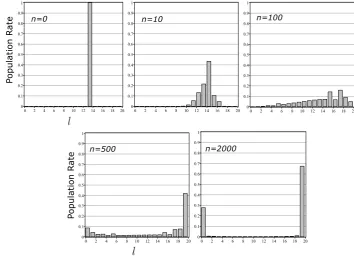
Figure1 shows the result of computational simulation with M = L = 2, |Ψ⟩ = √0.7|ψ1⟩+

√

0.3|ψ2⟩ (P1 = 0.7, P2 = 0.3 ), ν1|1 =

√

0.5 (ν_2|1 = √0.5) and ν1|2 =

√

0.45 (ν_2|2 = √0.55). The histograms of population rates of states with l−₂₀1 <|

⟨

ψ1|Ψ{j1,j2,···,jn}

⟩ |2 _≤ l

20 (l =1, 2,· · ·, 20)

are calculated in the case ofn=0, 10, 100, 500 and 2000. One can see that with increasingn, the state distribution approaches the goal of differentiation, i.e.,{{ψ1,ψ2},{0.7, 0.3}}.

P

opulat

ion R

ate

n=0 n=10 n=100

n=500 P opulat ion R ate n=2000

Figure 1. Histograms of population rates of states with l₂₀−1 < |

⟨

ψ1|Ψ{i1,i2,···,in} ⟩

|2 _≤ l

20 (l = 1, 2,· · ·, 20) in the case of n = 0, 10, 100, 500 and 2000. The parameters are set by M = L = 2,

|Ψ⟩=√0.7|ψ1⟩+

√

0.3|ψ2⟩(P1=0.7, P2=0.3 ),ν1|1=

√

0.5(ν_2|1=√0.5)andν_1|2=√0.45(ν_2|2=

√

0.55). IfΨ_{{i1,i2,···,in}}⟩≈ |ψ1⟩(|ψ2⟩),| ⟨

ψ1|Ψ{i1,i2,···,in} ⟩

|2_{takes a value nearby 1(0). With increasing}

n, the state distribution approaches to{{ψ1,ψ2},{0.7, 0.3}}.

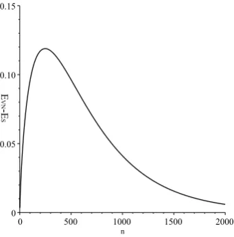
Figure2 shows the behavior of the state entropyD, von Neumann entropy and−log(Tr(ρ2))

for the distribution{Ψ_{i1,i2,···,in},P{i1,i2,···,in}}, which are calculated in the same setting of parameters.

entropyDtakes values close to von Neumann entropy at very largen. In fact, as shown in Figure3, the difference between von Neumann entropy and the state entropy is noticeable mostly at earlier stages. These results imply that state distributions appearing in the differentiation process are non-classical in general.

Figure 2. Behaviors of state entropy, von Neumann entropy and−log(Tr(ρ2))at the parameters of

M = L = 2, |Ψ⟩ = √0.7|ψ1⟩+

√

0.3|ψ2⟩ (P1 = 0.7, P2 = 0.3 ),ν1|1 =

√

0.5(ν_2|1 = √0.5)and

ν1|2=

√

0.45(ν_2|2=√0.55)

Figure 3.Difference between von Neumann entropy and state entropy.

7. Conclusions

The state entropy is a truly non-classical quantity because it depends not only on statistical probabilities, but also on similarities among states. The differentiation phenomenon is also non-classical, because it is interpreted as dynamics of the probabilities and similarities. Definition of the state entropy and modeling of the differentiation process are impossible in the framework of classical probability theory.

Author Contributions: Conceptualization, M.A., I.B. and A.K.; Methodology, M.A. and A.K.; Validation, I.B., E.M.P. and A.K.; Writing-Original Draft Preparation, M.A.; Writing-Review & Editing, I.B., E.M.P. and A.K.

Acknowledgments:I.B. was supported by Marie Curie Fellowship at City University of London, H2020-MSA-IF-2015, grant N 696331.

Conflicts of Interest:The authors declare no conflict of interest.

Appendix A. State Entropy and other Quantum Entropies

In this paper, we propose the state entropy,

D({⟨ρ⟩_Ψ

i,Pi}) =

N

∑

i=1

Pi(−log(Tr(ρ|Ψi⟩ ⟨Ψi|))).

More generally, it is defined as

D({⟨ρ⟩_Ψ

i,Pi}) =

N

∑

i=1

Pif(Tr(ρ|Ψi⟩ ⟨Ψi|)),

by using a convex and monotone decreasing function f(x). Mathematically,D({⟨ρ⟩_Ψ

i,Pi}depends

on the way of decomposition of ρ. As discussed in Section 5, for ρ = ∑_iN₌₁Pi|Ψi⟩ ⟨Ψi|,

f(Tr(ρ|Ψi⟩ ⟨Ψi|)) = f(⟨ρ⟩_Ψi)is interpreted as the degree of orthogonality between|Ψi⟩ ⟨Ψi|andρ. In

this sense,Devaluates a sort of diversity in the state distribution{Ψi,Pi}, and it takes the maximal

value equivalent to−Tr(ρlogρ)for the Schatten decomposition (see Equation (18)).

On the other hand, there are many mathematical expansions of von Neumann entropy. As examples, the quantum version of Rényi entropy [51],

Rα(ρ) = 1

1−αlog(Tr(ρ

α_{)), (A1)}

and the one of Tsallis entropy [52],

Tα(ρ) = 1

1−α(Tr(ρ

α_{)−1), (A2)}

are well-known. These entropies approach to von Neumann entropyS(ρ) =−Tr(ρlogρ)in the limit

α → 1. The index α, which is called the entropic parameter, is nonnegative andα ̸= 1. Further, such generalized entropies are uniformly represented in the form of quantum version of Salicrú entropy [53,54], which is given by

H_(h,ϕ)(ρ) =h(Trϕ(ρ)), (A3)

where the functionsh : R → Randϕ : [0, 1] → Rsatisfy either of the following conditions: (i)h is increasing andϕis concave; or (ii)his decreasing andϕis convex. In the form of Rényi entropy, h(x) =log_1−α(x)andϕ(x) =xα, and in the form of Tsallis entropy,h(x) = x−_1−α1andϕ(x) =xα. Of course, von Neumann entropy is also recovered ath(x) =xandϕ(x) =−xlogx.

Here, we have to point out thatH₍h,ϕ)(ρ)is practically calculated as

H(h,ϕ)(ρ) =h( M

∑

k=1

ϕ(λ_k)),

by using the eigenvalues ofρ, that is, any quantum entropic measure that is reduced into H(h,ϕ)(ρ)

does not depend on the way of decomposition of ρ. The state entropy is different in this point. Actually, it is clear thatD({⟨ρ⟩_Ψ

References

1. Von Neumann, J. Thermodynamik quantummechanischer Gesamheiten.Gott. Nach.1927,1, 273–291. 2. Von Neumann, J.Mathematische Grundlagen der Quantenmechanik; Springer: Berlin, Germany, 1932. 3. Horodecki, M.; Oppenheim, J.; Winter, A. Partial quantum information.Nature2005,436, 673–676.

4. Umegaki, H. Conditional expectations in an operator algebra IV (entropy and information). Kodai Math. Sem. Rep.1962,14, 59–85.

5. Ohya, M. Fundamentals of Quantum Mutual Entropy and Capacity.Open Syst. Inf. Dyn.1999,6, 69–78. 6. Asano, M.; Basieva, I.; Khrennikov, A.; Yamato, I. A model of differentiation in quantum bioinformatics.

Prog. Biophys. Mol. Biol.2017,130, 88–98.

7. Zurek, W.H. Decoherence and the Transition from Quantum to Classical.Phys. Today1991,44, 36–44. 8. Lindblad, G. On the generators of quantum dynamical semigroups.Commun. Math. Phys.1976,48, 119. 9. Gorini, V.; Kossakowski, A.; Sudarshan, E.C.G. Completely positive semigroups of N-level systems.J. Math. Phys.

1976,17, 821.

10. Khrennikov, A. Classical and quantum mechanics on information spaces with applications to cognitive, psychological, social and anomalous phenomena.Found. Phys.1999,29, 1065–1098.

11. Khrennikov, A. Quantum-like formalism for cognitive measurements.Biosystems2003,70, 211–233. 12. Khrennikov, A. On quantum-like probabilistic structure of mental information.Open Syst. Inf. Dyn. 2014,

11, 267–275.

13. Khrennikov, A. Information Dynamics in Cognitive, Psychological, Social, and Anomalous Phenomena; Ser.: Fundamental Theories of Physics; Kluwer: Dordreht, The Netherlands, 2004.

14. Busemeyer, J.B., Wang, Z., Townsend, J.T. Quantum dynamics of human decision making.J. Math. Psychol.

2006,50, 220–241.

15. Haven, E. Private information and the ‘information function’: A survey of possible uses.Theory Decis.2008,

64, 193–228.

16. Yukalov, V.I.; Sornette, D. Processing Information in Quantum Decision Theory. Entropy 2009, 11, 1073–1120.

17. Khrennikov, A.Ubiquitous Quantum Structure: From Psychology to Finances; Springer: Berlin/Heidelberg, Germany; New York, NY, USA, 2010.

18. Asano, M.; Masanori, O.; Tanaka, Y.; Khrennikov, A.; Basieva, I. Quantum-like model of brain’s functioning: Decision making from decoherence.J. Theor. Biol.2011,281, 56–64.

19. Busemeyer, J.R.; Pothos, E.M.; Franco, R.; Trueblood, J. A quantum theoretical explanation for probability judgment errors.Psychol. Rev.2011,118, 193–218.

20. Asano, M.; Ohya, M.; Khrennikov, A. Quantum-Like Model for Decision Making Process in Two Players Game - A Non-Kolmogorovian Model.Found. Phys.2011,41, 538–548.

21. Asano, M.; Ohya, M.; Tanaka, Y.; Khrennikov, A.; Basieva, I. Dynamics of entropy in quantum-like model of decision making.AIP Conf. Proc.2011,63, 1327.

22. Bagarello, F. Quantum Dynamics for Classical Systems: With Applications of the Number Operator; Wiley: New York, NY, USA, 2012; Volume 90, p. 015203.

23. Busemeyer, J.R.; Bruza, P.D.Quantum Models of Cognition and Decision; Cambridge Press: Cambridge, UK, 2012. 24. Asano, M.; Basieva, I.; Khrennikov, A.; Ohya, M.; Tanaka, Y. Quantum-like dynamics of decision-making.

Phys. A Stat. Mech. Appl.2010,391, 2083–2099.

25. De Barros, A.J. Quantum-like model of behavioral response computation using neural oscillators.

Biosystems2012,110, 171–182.

26. Asano, M.; Basieva, I.; Khrennikov, A.; Ohya, M.; Tanaka, Y. Quantum-like generalization of the Bayesian updating scheme for objective and subjective mental uncertainties.J. Math. Psychol.2012,56, 166–175. 27. De Barros, A.J.; Oas, G. Negative probabilities and counter-factual reasoning in quantum cognition. Phys.

Scr.2014,T163, 014008.

28. Wang, Z.; Busemeyer, J.R. A quantum question order model supported by empirical tests of an a priori and precise prediction.Top. Cogn. Sci.2013,5, 689–710.

29. Dzhafarov, E.N.; Kujala, J.V. On selective influences, marginal selectivity, and Bell/CHSH inequalities.

30. Wang, Z.; Solloway, T.; Shiffrin, R.M.; Busemeyer, J.R. Context effects produced by question orders reveal quantum nature of human judgments.PNAS2014,111, 9431–9436.

31. Khrennikov, A. Quantum-like modeling of cognition.Front. Phys.2015,3, 77.

32. Boyer-Kassem, T.; Duchene, S.; Guerci, E. Testing quantum-like models of judgment for question order effect.Math. Soc. Sci., 2016, 80, 33–46.

33. Asano, M.; Basieva, I.; Khrennikov, A.; Ohya, M.; Tanaka, Y. A Quantum-like Model of Selection Behavior.

J. Math. Psychol.2016, doi:10.1016/j.jmp.2016.07.006

34. Yukalov, V.I.; Sornette, D. Quantum Probabilities as Behavioral Probabilities.Entropy2017,19, 112. 35. Igamberdiev, A.U.; Shklovskiy-Kordi, N.E. The quantum basis of spatiotemporality in perception and

consciousnes.Prog. Biophys. Mol. Biol.2017,130, 15–25.

36. De Barros, J.A; Holik, F.; Krause, D. Contextuality and indistinguishability.Entropy2017,19, 435.

37. Bagarello, F.; Di Salvo, R.; Gargano, F.; Oliveri, F.(H,ρ)-induced dynamics and the quantum game of life.

Appl. Math. Mod.2017,43, 15–32.

38. Takahashi, K.S.-J.; Makoto, N. A note on the roles of quantum and mechanical models in social biophysics.

Prog. Biophys. Mol. Biol. 2017,130 (Pt A), 103–105.

39. Asano, M.; Basieva, I.; Khrennikov, A.; Ohya, M.; Tanaka, Y.; Yamato, I. Quantum-like model of diauxie in Escherichia coli: Operational description of precultivation effect.J. Theor. Biol.2012,314, 130–137.

40. Accardi, L.; Ohya, M. Compound channels, transition expectations, and liftings.Appl. Math. Optim. 1999,

39, 33–59.

41. Asano, M.; Basieva, I.; Khrennikov, A.; Ohya, M.; Tanaka, Y.; Yamato, I. A model of epigenetic evolution based on theory of open quantum systems.Syst. Synth. Biol.2013,7, 161.

42. Asano, M.; Hashimoto, T.; Khrennikov, A.; Ohya, M.; Tanaka, A. Violation of contextual generalization of the Leggett-Garg inequality for recognition of ambiguous figures.Phys. Scr.2014,2014, T163

43. Asano, M.; Basieva, I.; Khrennikov, A.; Ohya, M.; Tanaka, Y.; Yamato, I. Quantum Information Biology: From Information Interpretation of Quantum Mechanics to Applications in Molecular Biology and Cognitive Psychology.Found. Phys.2015,45, 1362.

44. Asano, M.; Khrennikov, A.; Ohya, M.; Tanaka, Y.; Yamato, I. Three-body system metaphor for the two-slit experiment andEscherichia colilactose-glucose metabolism.Philos. Trans. R. Soc. A2016, doi:10.1098/rsta.2015.0243. 45. Ohya, M.; Volovich, I.Mathematical Foundations of Quantum Information and Computation and its Applications

to Nano- and Bio-Systems; Springer: Berlin, Germany, 2011.

46. Asano, M.; Khrennikov, A.; Ohya, M.; Tanaka, Y.; Yamato, I.Quantum Adaptivity in Biology: From Genetics to Cognition; Springer: Berlin, Germany, 2015.

47. Oaksford, M.; Chater, N. A Rational Analysis of the Selection Task as Optimal Data Selection.Psychol. Rev.

1994,101, 608–631.

48. Pothos, E.M.; Chater, N. A simplicity principle in unsupervised human categorization.Cogn. Sci.2002,26, 303–343.

49. Miller, G.A. Free Recall of Redundant Strings of Letters.J. Exp. Psychol.1958,56, 485–491.

50. Jamieson, R.K.; Mewhort, D.J.K. The influence of grammatical, local, and organizational redundancy on implicit learning: An analysis using information theory.J. Exp. Psychol. Learn. Mem. Cogn.2005,31, 9–23. 51. Rényi., A. On measures of entropy and information. In Proceedings of the 4th Berkeley Symposium on

Mathematical Statistics and Probability, Berkeley, CA, USA, 20–30 July 1960; Volume 1, p. 547. 52. Tsallis, C. Possible generalization of Boltzmann–Gibbs statistics.J. Stat. Phys.1988,52, 479 .

53. Salicrú, M.; Menéndez, M.L.; Morales, D.; Pardo, L. Asymptotic distribution of (h,ϕ)-entropies.

Commun. Stat. Theory Methods1993,22, 2015.

54. Bosyk, G.M.; Zozor, S.; Holik, F.; Portesi, M.; Lamberti, P.W. A family of generalized quantum entropies: definition and properties.Quantum Inf. Proc.2016,15, 3393–3420.

c