Coarse-grained simulation of DNA using LAMMPS : an implementation of the oxDNA model and its applications

DOI 10.1140/epje/i2018-11669-8 Regular Article

P

HYSICAL

J

OURNAL

E

Coarse-grained simulation of DNA using LAMMPS

An implementation of the oxDNA model and its applications

Oliver Henrich1,a, Yair Augusto Guti´errez Fosado2, Tine Curk3,4, and Thomas E. Ouldridge5,6

1

Department of Physics, SUPA, University of Strathclyde, Glasgow G4 0NG, Scotland, UK

2

School of Physics and Astronomy, University of Edinburgh, Edinburgh EH9 3FD, Scotland, UK

3

CAS Key Laboratory of Soft Matter Physics, Beijing National Laboratory for Condensed Matter Physics, Institute of Physics, Chinese Academy of Sciences, Beijing 100190, China

4

Department of Chemistry, University of Cambridge, Cambridge CB2 1EW, UK

5

Department of Bioengineering, Imperial College London, London SW7 2AZ, UK

6

Centre of Synthetic Biology, Imperial College London, London SW7 2AZ, UK Received 20 February 2018 and Received in final form 13 April 2018 Published online: 10 May 2018

c

The Author(s) 2018. This article is published with open access at Springerlink.com

Abstract. During the last decade coarse-grained nucleotide models have emerged that allow us to study DNA and RNA on unprecedented time and length scales. Among them is oxDNA, a coarse-grained, sequence-specific model that captures the hybridisation transition of DNA and many structural prop-erties of single- and double-stranded DNA. oxDNA was previously only available as standalone software, but has now been implemented into the popular LAMMPS molecular dynamics code. This article describes the new implementation and analyses its parallel performance. Practical applications are presented that focus on single-stranded DNA, an area of research which has been so far under-investigated. The LAMMPS implementation of oxDNA lowers the entry barrier for using the oxDNA model significantly, facilitates fu-ture code development and interfacing with existing LAMMPS functionality as well as other coarse-grained and atomistic DNA models.

1 Introduction

DNA is one of the most important bio-polymers, as its sequence encodes the genetic instructions needed in the development and functioning of many living organisms. While we know now the sequence of many genomes, we still know little as to how DNA is organised in 3D inside a living cell, and of how gene regulation and DNA function are coupled to this structure. The complexity of the DNA molecule can be brought to mind by highlighting a few of its quantitative aspects. The entire DNA within a single human cell is about 2 m long, but only 2 nm wide and or-ganised at different hierarchical levels. If compressed into a spherical ball, this ball would have a diameter of about 2μm [1].

Computational modelling of DNA appears as the only avenue to understanding its intricacies in sufficient detail and has been an important field in biophysics for decades. Traditionally, most of the available simulation techniques have worked at the atomistic level of detail [2]. Existing

Contribution to the Topical Issue “Advances in Computa-tional Methods for Soft Matter Systems” edited by Lorenzo Rovigatti, Flavio Romano, John Russo.

a _e-mail:

[email protected]

atomistic force fields can capture fast conformational fluc-tuations and protein-DNA binding, but cannot deliver the necessary temporal and spatial resolution to describe phe-nomena that occur on larger time and length scales as they are often limited to a few hundred base pairs and (at most) microsecond time scales. Recent years have there-fore witnessed a rapid increase of a new research effort at a different, coarse-grained level [3]. Coarse-grained (CG) models of DNA can provide significant computational and conceptual advantages over atomistic models leading often to three or more orders of magnitude greater efficiency. The challenge consists in retaining the right degrees of freedom so that the CG model reproduces relevant emer-gent structural features and thermodynamic properties of DNA. CG modelling of DNA is not only an efficient al-ternative to atomistic approaches. It is indispensable for the modelling of DNA on time scales in the millisecond range and beyond, or when long DNA strands of tens of thousands of base pairs or more have to be considered, e.g.to study the dynamics of DNA supercoiling (i.e., the local over- or under-twisting of the double helix, which is also important for gene expression in bacteria), of genomic DNA loops and of chromatin or chromosome fragments.

into top-down approaches, which use empirical inter-actions that are parameterised to match experimental observables, or bottom-up approaches, which eliminate dispensable degrees of freedom systematically starting from atomistic force fields. They may also target dif-ferent applications depending on their capabilities, such as single- versus double-stranded DNA (ssDNA and dsDNA), or nanotechnological versus biological applica-tions. We refer to [4] for a comprehensive overview of the capabilities of individual models and recent activities in this field.

From a software point of view these models are often based on standalone software [5–7], which has a some-what limiting effect on uptake and user communities growth. Others models use popular MD-codes as com-putational platforms, such as GROMACS [8] in case of the SIRAH [9] and the MARTINI force field [10], or NAMD [11, 12]. Another suitable platform for CG sim-ulation of DNA has emerged in form of the powerful Large-Scale Atomic/Molecular Massively Parallel Simula-tor (LAMMPS) for molecular dynamics [13], including the widely used 3SPN.2 model [14, 15] and others that target even larger length scales [16, 17].

This article reports the latest effort of implementing the popular oxDNA model [18, 19] into the LAMMPS code. Until recently this model was only available as bespoke and standalone software [20]. Through the effi-cient parallelisation of LAMMPS it is now possible to run oxDNA in parallel on multi-core CPU-architectures, ex-tending its capabilities to unprecedented time and length scales. The largest system that could be studied by oxDNA was previously limited by the size of system that can be fitted onto a single GPU.

This paper is organised as follows: in sect. 2 we briefly introduce the details of the oxDNA and oxDNA2 models. Section 3 explains how the LAMMPS implementation of the oxDNA models can be invoked and provides further information on the code distribution and documentation. In sect. 4 we describe the LAMMPS implementation of novel Langevin-type rigid-body integrators which feature improved stability and accuracy. Section 5 gives details of the scaling performance of parallel implementation. Sec-tion 6 presents results on the behaviour of single-stranded DNA, an area of DNA research which so far has not been intensively investigated. One application is concerned with lambda-DNA of a bacteriophage, whereas the other appli-cation involves a plasmid cloning vector pUC19. In sect. 7 we summarise this work.

2 The oxDNA model

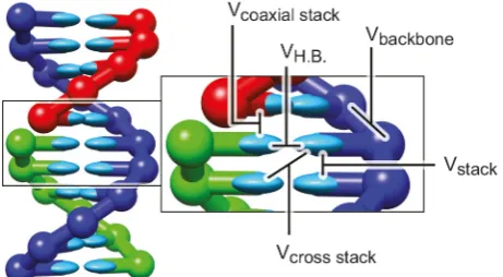
The oxDNA model consists of rigid nucleotides with three interaction sites for the effective interactions between the nucleotides. These pairwise-additive forces arise due to the excluded volume, the connectivity of the phosphate backbone, the stacking, cross-stacking and coaxial stack-ing as a consequence of the hydrophobicity of the bases, as well as hydrogen bonding between complementary base pairs. Figure 1 illustrates these interactions schematically

Fig. 2. (a) Schematic distinction between oxDNA (left) and oxDNA2 (right). In oxDNA all interaction sites are co-linear whereas in oxDNA2 the backbone interaction site and the stacking and hydrogen-bonding interaction sites are oriented at an angle. (b) The non-co-linear arrangement of the inter-action sites leads to the formation of the major and minor groove, an important structural feature of DNA. Reproduced from [24], with the permission of AIP Publishing.

A short schematic overview of various interactions in-volved in the definition of oxDNA model is given in fig. 1. More details can be found in the original publications [18, 19].

The original model (oxDNA) has been further devel-oped to include sequence-specific stacking and hydrogen bonding interaction strengths [25] (oxDNA1.5) and im-plicit ions, which are modelled by means of a Debye-H¨uckel potential [24] (oxDNA2). A major improvement of the latest version is also the fact that it shows the correct structure with major and minor grooves (see fig. 2(b)). This is achieved through a modification of the relative position of the backbone and stacking/hydrogen bonding interaction sites, as schematically depicted in fig. 2(a).

3 The LAMMPS implementation of oxDNA

3.1 Code distribution, force fields and compilation

The software is open source and distributed under GNU General Public License (GPL). It is available for download as LAMMPS USER-package from the central LAMMPS repository at Sandia National Laboratories, USA [13]. This includes a detailed online documentation, examples and utility scripts. We refer also to these materials for a general introduction into the usage of LAMMPS.

To compile the code, load the LAMMPS standard packages MOLECULE and ASPHERE and the USER-CGDNA package by issuing

make yes-molecule yes-asphere yes-user-cgdna

in the main source code directory and compile as usual.

All three versions oxDNA, oxDNA1.5 and oxDNA2 are implemented in the LAMMPS code and can be invoked through appropriate keywords in the input file. This al-lows for instance to run without sequence-specific inter-actions and without implicit ions (oxDNA force field and keyword seqav ≡ oxDNA), with sequence-specific inter-actions and without implicit ions (oxDNA force field and keyword seqdep ≡oxDNA1.5) or with implicit ions and with or without sequence-specific interactions (oxDNA2 force field and keywords seqdeporseqav, respectively).

The source code is also distributed via our main repos-itory at CCPForge [26] under the project name Coarse-Grained DNA Simulation (cgdna). Please send a request to join the project for full access that includes permission to browse the repository and commit changes.

3.2 Force and torque calculation

Integrating the equations of motion of rigid bodies requires accurate information of their relative orientations. In sim-ple situations this can be achieved through Euler angles, which describe the orientation of a rigid body and its lo-cal reference frame with respect to the laboratory system. Euler angles have the disadvantage that they are not un-ambiguously defined as a singularity arises when two ro-tation axes fall parallel. This situation, usually referred to as gimbal lock, arises easily in a system that contains a large number of rigid bodies. Unsurprisingly, it triggers numerical instabilities, which is why rigid-body problems are best formulated by means of quaternions [27] instead of Euler angles.

Computationally it is most efficient to integrate the quaternion degrees of freedom directly via a generalised 4-component quaternion torque (see [19] for a detailed derivation of the oxDNA forces and generalised 4-torques using quaternion dynamics). Unfortunately such an inter-face for generalised quaternion torques and momenta is not provided in LAMMPS. It expects for its rigid-body integrators 3-component torques and angular momenta as input quantities (besides the Newtonian force for the inte-gration of the coordinate degrees of freedom). To be con-sistent and simplify interfacing with existing functionality, we decided to adhere to this convention. This, however, entails conversion of the unit quaternions into Cartesian unit vectors of a body frame before forces and torques can be calculated for the integration step, thus leading to a computational overhead (see appendix A).

Once this choice has been made, the calculation of the forces and torques is most conveniently formulated follow-ing ref. [28]. If ˆaand ˆbare the principal axes of two rigid bodies A and B andris the norm of the relative distance vectorr=rA−rB from B to A, then the pair potential depends on a combination of these quantities

U =U

r,aˆ,ˆb

=U

r,{aˆm·rˆ},

ˆ

bn·rˆ

,

ˆ

am·ˆbn

,

as

FA=−FB=−

∂U ∂r =

−∂U ∂rrˆ−r

−1

m

∂U ∂(ˆam·r)

ˆ

a⊥_m+ ∂U

∂(ˆbm·r) ˆ

b⊥_m

.

(2)

Here ˆa⊥_m= ˆam−(ˆam·rˆ) ˆrdenotes the component of ˆam which is perpendicular to ˆr. The torques are slightly more involved:

τA=

m

∂U ∂(ˆam·r)

ˆ

r×aˆm

−

mn

∂U ∂(ˆam·bˆn)

ˆ

am×bˆn

, (3)

τB =

n

∂U ∂(ˆbn·r)

ˆ

r×bˆn

+

mn

∂U ∂(ˆam·bˆn)

ˆ

am×bˆn

. (4)

The fact that local angular momentum conservation re-quires

τA+τB+r×f = 0 (5) can be conveniently utilised for debugging and verification purposes. The implementation was verified against two independent implementations, namely Ouldridge’s own code, which is based on quaternion dynamics [19] as well as the standalone oxDNA code [20], which makes also use of the same scheme for the force and torque calculation. To this end two benchmarks were studied, a 5-base-pair duplex and a 8-base-pair nicked duplex, which are both provided as examples in the USER-CGDNA package.

3.3 Input file

In the following we discuss the structure of the input file and how the newly introduced oxDNA classes are invoked. We work with Lennard-Jones reduced units, which are invoked in LAMMPS via

units lj

The system is three-dimensional:

dimension 3

In LAMMPS, an oxDNA nucleotide is represented as a bonded-ellipsoidal hybrid particle with the associated de-grees of freedom of bonded particles in a bead-spring poly-mer (backbone connectivity) and aspherical particles with shape (moment of inertia), quaternion (orientation) and angular momentum:

atom style hybrid bond ellipsoid

Users are required to suppress the atom sorting algorithm as this can lead to problems in the bond topology of the DNA:

atom modify sort 0 1.0

It is important to set the skin size correctly, which controls the extent of the neighbour lists. Too large a skin size and neighbour lists become unnecessarily long, leading to superfluous communication. Too short and partners in the pair interactions will be lost:

neighbor 1.0 bin

A good way to fine-tune this parameter is to run an NVE simulation with constant energy before applying Langevin integrators. We recommend neighbor 2.0 binas a safe starting point. Likewise, frequent update of the neighbour lists can lead to an undue performance degradation. This parameter should be tuned as well so that no dangerous builds (as reported in the standard output of LAMMPS) occur:

neigh modify every 1 delay 0 check yes

The initial configuration and topology is created by means of an external setup tool (see sect. 3.4) and read in:

read data data file name

All masses are set to 3.1575 in LJ units:

set atom * mass 3.1575

Note that the moment of inertia is determined through the shape parameter in the data file (see below sect. 3.4). There are four types of nucleotides (A = 1, C = 2, G = 3, T = 4), which are grouped together into a group named allfor the integration:

group all type 1 4

The new oxDNA classes with its parameters are invoked as follows:

bond style oxdna2/fene bond coeff * 2.0 0.25 0.7564

pair style hybrid/overlay oxdna2/excv & oxdna2/stk oxdna2/hbond oxdna2/xstk & oxdna2/coaxstk oxdna2/dh

pair coeff * * oxdna2/excv 2.0 0.7 0.675 2.0 & 0.515 0.5 2.0 0.33 0.32

pair coeff * * oxdna2/stk seqdep 0.1 6.0 0.4 & 0.9 0.32 0.6 1.3 0 0.8 0.9 0 0.95 0.9 0 & 0.95 2.0 0.65 2.0 0.65

pair coeff * * oxdna2/hbond seqdep 0.0 8.0 & 0.4 0.75 0.34 0.7 1.5 0 0.7 1.5 0 0.7 1.5 & 0 0.7 0.46 3.141592653589793 0.7 4.0 & 1.5707963267948966 0.45 4.0 &

1.5707963267948966 0.45

pair coeff 1 4 oxdna2/hbond seqdep 1.0678 8.0 & 0.4 0.75 0.34 0.7 1.5 0 0.7 1.5 0 0.7 1.5 & 0 0.7 0.46 3.141592653589793 0.7 4.0 & 1.5707963267948966 0.45 4.0 &

1.5707963267948966 0.45

pair coeff 2 3 oxdna2/hbond seqdep 1.0678 8.0 & 0.4 0.75 0.34 0.7 1.5 0 0.7 1.5 0 0.7 1.5 & 0 0.7 0.46 3.141592653589793 0.7 4.0 & 1.5707963267948966 0.45 4.0 &

1.5707963267948966 0.45

1.7 1.0 0.68 1.7 1.0 0.68 1.5 0 0.65 1.7 & 0.875 0.68 1.7 0.875 0.68

pair coeff * * oxdna2/coaxstk 58.5 0.4 0.6 & 0.22 0.58 2.0 2.891592653589793 0.65 1.3 & 0 0.8 0.9 0 0.95 0.9 0 0.95 40.0 &

3.116592653589793

pair coeff * * oxdna2/dh 0.1 1.0 0.815

Please note that according to the LAMMPS parsing rules the ampersands (&) represent line breaks.

Visit the LAMMPS online documentation and manual for more information and for information on oxDNA2.

3.4 Data file and setup tool

The data file contains all relevant structural parameters for the simulation,i.e.details about the number of atoms, the topology of the molecules, the size of the simulation box, initial velocities, etc. The LAMMPS implementation of oxDNA follows the standard form as discussed in the LAMMPS user manual. We outline the relevant parts be-low.

At the beginning of the data file the total number of particles and bonds has to be given. As we are using hybrid particles, we need to set the same number of ellipsoids. For a standard DNA duplex consisting of 8 complementary base pairs we need 16 atoms, 16 ellipsoids and 14 bonds, 7 on each of the two single strands. If the strands are nicked, which we do not assume here, the number of bonds would be reduced:

16 atoms 16 ellipsoids 14 bonds

We use four atom types to represent the four different nucleotides in DNA (A = 1, C = 2, G = 3, T = 4). We use only one bond type:

4 atom types 1 bond types

The dimensions of the simulation box are defined as fol-lows:

-20.0 20.0 xlo xhi -20.0 20.0 ylo yhi -20.0 20.0 zlo zhi

Although already stated in the input file, we need to pro-vide again the masses of the nucleotides:

Masses 1 3.1575 2 3.1575 3 3.1575 4 3.1575

The nucleotides are defined after the keywordAtoms. Each row contains the atom-ID (1, 2, 3 in the example below), the atom type (1,1,4), the position (x, y, z), the molecule ID (all 1 in this case), an ellipsoidal flag (1) and a density (1):

Atoms

1 1 0.00000 0.00000 0.00000 1 1 1 2 1 0.13274 -0.42913 0.37506 1 1 1 3 4 0.48461 -0.70835 0.75012 1 1 1 .

. .

Next we set the initial velocities to the desired value, here all equal to 0. The first column contains the atom-ID (1,2,3), the following three columns the translational, and the last three columns the angular velocity:

Velocities

1 0.0 0.0 0.0 0.0 0.0 0.0 2 0.0 0.0 0.0 0.0 0.0 0.0 3 0.0 0.0 0.0 0.0 0.0 0.0 .

. .

Note that this is our special choice in the setup tool. The velocities can be generally initialised to any value. Large values will lead to the FENE springs becoming over-stretched and may provoke an early abortion of the run.

The ellipsoids are defined with atom-ID, shape (1.17398 to produce the correct moment of inertia) and initial quaternion (last four columns):

Ellipsoids

1 1.17398 1.17398 1.17398 1.00000 0. 0. 0. 2 1.17398 1.17398 1.17398 0.95534 0. 0. 0.29552 3 1.17398 1.17398 1.17398 0.82534 0. 0. 0.56464 .

. .

Finally, we specify the bond topology. The first column contains the bond-ID (1,2,3), the second one the bond type (1) and the third and fourth the IDs of the two bond partners:

Bonds 1 1 1 2 2 1 2 3 3 1 3 4 . . .

To simplify the setup procedure we provide a simple python tool with the example and utility files of the USER-CGDNA package. The script allows the user to cre-ate single- and double-stranded DNA from an input file that specifies the sequence and requires an installation of numpy.

The syntax is very straightforward, but the system size has to be specified in the following way:

$> python generate.py <box offset> \

<cubic box length> <sequence file name>

The output is written directly into a data file in LAMMPS format. This has to be given in the LAMMPS input file. <sequence file name> is an ASCII input file that con-tains keywords and the sequence of one ssDNA strand. Two options are available. For a single, helical strand con-sisting of ssDNA, the sequence file contains a single line:

If the sequence is prepended by the keywordDOUBLE, then a single, helical DNA duplex is created. The bases on the second strand are complementary to those on the first strand, which is given in the sequence input file:

DOUBLE ACGTA

Consecutive strands are positioned and oriented randomly without creating any overlap in case of more than one ssDNA or dsDNA strand. Note that the procedure works only below a critical density as this simple script does not feature cell lists. Besides these setup tools, the USER-CGDNA package contains as well example input, data and standard output files of short benchmark runs of dsDNA duplexes.

3.5 Output and visualisation

LAMMPS offers a multitude of possible output formats, including parallel HDF5 and NetCDF formats, VTK for-mat or very basic standard trajectory data. We will sum-marise here how output of basic observables of the oxDNA model can be invoked in the input file.

The xyz style writes XYZ files, which is a simple text-based coordinate format that many codes can read, which has one line per atom with the atom type and thex-,y-, andz-coordinate of that atom. This style is invoked via

dump 1 all xyz Nint trajectory.xyz

where Nint is the output frequency in timesteps. Addi-tional output of,e.g., velocity, force and torque on a per-atom basis makes some customisation necessary,

dump 2 all custom Nint filename.dat id x y z & vx vy vz fx fy fz tqx tqy tqz

where id is the unique atom-ID. The output of quater-nions requires a so-calledcomputestyle. The result of the computestyle can then be retrieved in the following way:

compute quat all property/atom quatw quati & quatj quatk

dump 3 all custom Nint filename.dat id & c quat[1] c quat[2] c quat[3] c quat[4]

Another observable that may be of interest is the en-ergy, or more specifically broken down into rotational, ki-netic and potential energy. This is also done through a computestyle:

compute erot all erotate/asphere compute ekin all ke

compute epot all pe

variable erot equal c erot variable ekin equal c ekin variable epot equal c epot

variable etot equal c erot+c ekin+c epot

Note that the somewhat simpler thermo style com-mand for output discards the kinetic energy of rotation when the kinetic energy is requested.

LAMMPS does not contain a direct visualisation toolkit. There are, however, a multitude of ways how

snapshots can be visualised. ParaView [29] for instance, is an open source, multi-platform data analysis and vi-sualisation application. The images in this work have been generated with the molecular visualisation program VMD (Visual Molecular Dynamics) [30]. More informa-tion about possible visualisainforma-tion pipelines can be found in the LAMMPS online manual [13].

4 Langevin-type rigid-body integrators

Together with the USER-CGDNA package comes also an implementation of novel Langevin-type rigid-body inte-grators that were developed by Davidchack, Ouldridge and Tretyakov [31]. The motivation for this was that previ-ously only a limited choice of suitable Langevin integra-tors for rigid bodies was available in LAMMPS. Without noise all integrators A, B and C in the above reference are identical and basically equivalent to the integrator pre-sented by Miller et al.[32]. Nevertheless, we refer to this case as the “DOT integrator” (the other implementation of the Miller integrator is only available when using the fix rigid command in LAMMPS). The DOT integra-tor is an alternative to the standard LAMMPS NVE in-tegrator for aspherical particles, and can be invoked by replacing the standard choice

fix 1 all nve/asphere

with

fix 1 all nve/dot

in the input file. This energy-conserving integrator is use-ful for an analysis of the accuracy of this family of inte-grators or the integrity of the pair interactions at a given timestep sizeΔt.

The C integrator in ref. [31], to which we refer as “DOT-C integrator”, is invoked by replacing the stan-dard NVE integrator for aspherical particles and the fix for Langevin dynamics

fix 1 all nve/asphere

fix 2 all langevin 0.1 0.1 0.03 457145 angmom 10

with one single fix

fix 1 all nve/dotc/langevin 0.1 0.1 0.03 & 457145 angmom 10

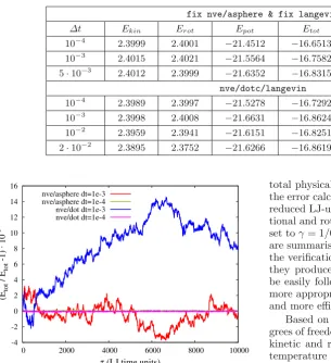
To measure the accuracy of the new integrators, we run a test case consisting of a short, nicked duplex with 8 base pairs (16 nucleotides). Figure 3 shows the accuracy measured through the normalised difference between the total energy Etot for this particular benchmark and the total energy at the beginning of the run Etot∗ . We com-pared the standard fix nve/asphere integrator, which is based on a Richardson iteration in the update of the quaternion degrees of freedom, to the new DOT integra-tor, which uses a rotation sequence to update the quater-nions. Shown are results for two different timestep sizes

Table 1.Average kinetic, rotational, potential and total energy for the standard LAMMPS integratorfix nve/asphere & fix

langevinand the DOT-C integratornve/dotc/langevinfor different timestep sizes.

fix nve/asphere & fix langevin

Δt Ekin Erot Epot Etot Standard error ofEtot fit

10−4 2.3999 2.4001 −21.4512 −16.6513 ±0.00377 (0.0227%) 10−3 _{2.4015 2.4021 −21.5564 −16.7582 ±0.00349 (0.0208%)}

5·10−3 2.4012 2.3999 −21.6352 −16.8315 ±0.00322 (0.0191%) nve/dotc/langevin

10−4 2.3989 2.3997 −21.5278 −16.7292 ±0.00362 (0.0216%) 10−3 _{2.3998 2.4008 −21.6631 −16.8624 ±0.00335 (0.0199%)}

10−2 2.3959 2.3941 −21.6151 −16.8251 ±0.00318 (0.0189%) 2·10−2 2.3895 2.3752 −21.6266 −16.8619 ±0.00313 (0.0185%)

-4 -2 0 2 4 6 8 10 12 14 16

0 2000 4000 6000 8000 10000

(E

tot

/ E

* tot

-1) · 10

-5

τ (LJ time units) nve/asphere dt=1e-3

nve/asphere dt=1e-4 nve/dot dt=1e-3 nve/dot dt=1e-4

Fig. 3. Relative normalised accuracy (Etot −Etot∗ )/Etot∗ of the standard LAMMPS NVE integrator for aspherical parti-cles and the NVE DOT integrator from ref. [31]. Etot∗ is the total free energy at the beginning of the simulation runs.

the same physical simulation time to allow direct compari-son of the deviations of a dynamical run. As this is done in the NVE ensemble and without noise, the energy should be exactly conserved. This corresponds to a straight, hor-izontal line at 0.

It is obvious that above a certain timestep size the ac-curacy of the new DOT integrator is slightly inferior com-pared to the standard integrator. Up to a certain point the DOT integrator actually seems to deviate further from the correct result, whereas the standard integrator fluctuates more around the correct value. This, however, is more or less a transient effect as longer runs show there is no per-manent drift away from the correct result. For Langevin dynamics, it is not possible to evaluate the accuracy and stability in the same way. We opted instead for an esti-mate based on the average kinetic, rotational, potential and total energy of the benchmark. Again, we performed runs of τ = 10000 Lennard-Jones time units length, this time thermalised, and averaged the results over the time interval. The number of MD-timesteps and the output fre-quency for each timestep size were adapted so that the

total physical simulation time and the statistical basis of the error calculations were consistent. The temperature in reduced LJ-units was set toT = 0.1, whereas the transla-tional and rotatransla-tional friction or damping coefficients were set toγ= 1/0.03 andΓ = 1/0.3, respectively. The results are summarised in table 1. These values were used during the verification of the LAMMPS implementation because they produced relatively smooth trajectories that could be easily followed. For actual production runs it may be more appropriate to use different values to allow a better and more efficient sampling of the configuration space.

Based on three translational and three rotational de-grees of freedom per nucleotide and 8 base pairs we expect kinetic and rotational energies Ekin = Erot = 2.4 for a temperature settings T = 0.1. This is very well achieved for all timestep sizes and both integrators, the standard LAMMPS integratorfix nve/asphere & fix langevin and the DOT-C integrator fix nve/dotc/langevin. However, there appears to be a slight decrease in the DOT-C integrator for very large step sizes (Δt= 2·10−2_{). The} deviation of the total energy between all timestep sizes, admittedly anad hoccriterion to quantify the stability of the integrators, but one that is rather hard for the inte-grators to get exactly right, is in the sub-percent range. It is actually slightly better for the DOT-C integrator than for the standard LAMMPS integrator. The statistical er-rors, reported in table 1, are the standard deviations of a linear least square fit and show that the deviations are well above the uncertainty of the fits.

Remarkably, for the DOT-C integrator the limit for a stable integration isΔt= 2·10−2_{, which represents a very} large timestep size. This is about 4 times larger than the maximum timestep size for which the standard LAMMPS Langevin integrator produces sound results. Because of the more complex rotations in quaternion space and vari-ous additional transformations that the DOT-C integrator requires there is a small overhead of about 15% compared to the standard LAMMPS integrator. Nevertheless, this small overhead of the DOT-C integrator is very well com-pensated by the computational efficiency and possibility to increase the timestep size by 400% (from a maximum ofΔt= 5·10−3for the standard LAMMPS integrator to

Fig. 4. The low-density benchmark consisting of a 10×10 array of DNA duplexes with A-T base pairs and a length of 600 base pairs each, in total 60 kbp. The high-density benchmark (not shown) consisted of a similar 40×40 array of duplexes with 960 kbp in total. The pictures show the final configuration the end of a performance run and were produced with VMD. The centre of mass of each nucleotide is represented through a sphere.

5 Performance analysis

We devised a few simple benchmarks to study the par-allel performance of the LAMMPS implementation. The size of each benchmark is well beyond the current capa-bilities of the standalone version, so each demonstrates as well a minimal performance requirement. The benchmarks consisted of arrays of double-stranded, regularly arranged DNA duplexes, each with a length of 600 base pairs. The low-density (LD) benchmark was formed by a 10×10 ar-ray of duplexes, giving a total of 60 kbp, and is shown in fig. 4. The high-density (HD) benchmark was formed by a 40×40 array of duplexes with a density 16 times larger than the LD case and a total number of 960 kbp. Whilst a regular array of double-stranded DNA strands appears perhaps somewhat artificial, it creates a reasonably load-balanced situation and facilitates the performance analy-sis. The obtained densities of DNA, are however very well comparable to those of DNA gels [33] and high-density states of DNA which form liquid-crystalline phases [34].

Strong scaling tests were performed on ARCHER on up to 86 nodes (LD) and 683 nodes (HD), respectively. The benchmark cases were run for 30,000 (LD) and 10,000 (HD) MD-timesteps with a timestep size ofΔt= 5×10−3_. We used the standard LAMMPS integrators for Langevin dynamics, although the scaling behaviour was found to be virtually identical when using the above described rigid-body integrator DOT-C. The primary reason for this was that the wallclock time for runs with the standard integra-tor was still a few percent shorter, although the improved efficiency of the DOT-C integrator would mean these runs were shorter in physical time. The temperature in reduced LJ-units was T = 0.1, whereas the translational and ro-tational friction coefficients were set to γ = 1/0.03 and

Γ = 1/0.3, respectively.

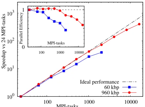
Figure 5 shows the parallel speedup for both bench-marks relative to the single node performance with 24 MPI-tasks. The code performs well for the LD

bench-100 101 102 103

100 1000 10000

Speedup vs 24 MPI-tasks

MPI-tasks

Ideal performance 60 kbp 960 kbp 0

1

100 1000 10000

Parallel Efficiency MPI-tasks

Fig. 5. Strong scaling behaviour: speedup of the low- and high-density benchmarks of 60 kbp and 960 kbp, respectively, compared to the single node performance with 24 MPI-tasks. The inset shows the parallel efficiency relative to the single node case with 24 MPI-tasks.

mark up to about 128 MPI-tasks with a parallel efficiency around 95% (see the inset). Beyond several hundred MPI-tasks a gradual performance degradation is observed. At 2048 MPI-tasks the parallel efficiency has decreased to about 45% and the total speedup is roughly 930-fold com-pared to the single core performance (39-fold comcom-pared to the single node performance).

A look at the ratio of the number of local atoms,i.e. those that are inside a process boundary, to the number of ghost atoms,i.e.those which need to be communicated via neighbour lists, proves that the observed performance degradation is due to the comparably small size of the problem. At the largest core counts there are on aver-age only about 60 local atoms present on each process, whereas the number of ghost atoms is with about 225 atoms almost four times larger. LAMMPS is known to re-quire at least a few hundred local atoms or more for a good parallel performance [35]. The speedup is still rela-tively good because the fraction of time that the algorithm spends in the force calculation is still comparably large. For the HD benchmark, 16 times larger than the LD case, the performance degradation is more or less mirrored at core counts that are about 16 times larger. For the HD benchmark the total speedup at 16384 MPI-tasks is 9680-fold with respect to the single core performance (400-9680-fold compared to the single node performance) and the parallel efficiency is still at around 60%.

architectures such as many-core chips and general purpose graphical processing units (GPGPUs).

One of the major advantages of the new LAMMPS implementation is that it can be directly compared with other coarse-grained models that are also based on the LAMMPS code. To this end, we compared the single core performance of oxDNA2 with that of 3SPN.2 [14]. The benchmark consisted of two complementary dsDNA du-plexes of 8 bps with implicit ions. In order to compare both models we set the translational friction coefficient γ to about (300 fs)−1. We opted for the maximum timestep size that provided a stable integration, which was Δt= 35 fs (3SPN.2) andΔt= 48 fs (oxDNA2 + DOT-C integrator), respectively.

On a single Intel Core i7 2.8 GHz processor using the latest version of LAMMPS (16 March 2018) 3SPN.2 deliv-ered a performance of about 60μs per day. oxDNA2 was able to surpass this by about a factor 1.6 with a perfor-mance of roughly 100μs per day. Note that comparing the wall times is only an approximate way to compare the per-formance as there is no guarantee that similar processes take a similar simulation time in the two models.

Apart from the enhanced stability of the rigid-body integrator, this difference in performance will be caused by the different number of degrees of freedom that both models require: oxDNA/oxDNA2 uses only 13 degrees of freedom per nucleotide (3 coordinate positions, 3 trans-lational momenta, 3 angular momenta and 4 quaternion degrees of freedom), whereas 3SPN.2 uses 18 degrees of freedom per nucleotide (3 particles with each 3 coordinate positions and translational momenta).

Unfortunately, we could not measure the parallel per-formance of 3SPN.2. But this conceptual difference be-tween the two models is very likely to entail further detri-mental effects when running in parallel. With the larger number of degrees of freedom per nucleotide in 3SPN.2, communication overheads are likely to build up more quickly and neighbour lists are longer and probably have to be rebuilt more frequently. On the other hand, the cur-rent LAMMPS implementation of oxDNA offers further potential for optimisation as it spends a good part its time computing the inverse cosine (around 12%, see ap-pendix A). This could be alleviated for instance through the introduction of appropriate lookup tables for trigono-metric functions.

6 Applications

The structural properties of DNA such as the persis-tence length, radius of gyration and torsional rigidity play an important role in its function. Characterising these properties and their dependence on different conditions is therefore fundamental for highly complex processes such as DNA packaging, replication and denaturation. Exper-imentally, however, making these measurements is not an easy task as it requires subtle manipulation of single molecules and direct measurement of their response to ap-plied forces or displacements, which can then be related

to the elasticity of DNA. By using coarse-grained compu-tational models like oxDNA, we can study these systems in more detail. These simulations can in turn provide in-sights into experimental data or the performance of other theoretical approaches.

The radius of gyration is a particularly useful descrip-tor of the structure and compactness of macromolecules. For ssDNA the radius of gyrationRg can be defined as

R2_g= 1

N

N

i=1

(ri−r¯)2, (6)

where N is the number of nucleotides,ri is the position of the i-th nucleotide and ¯r = 1

N

N

i=1ri is the mean position of the ssDNA strand. For dsDNA this definition would be modified to use the centre-of-mass coordinate of a base pair (bp) andNwould be replaced with the number of base pairs.

In this section we present results obtained with the oxDNA2 model for two different systems: a sequence of ssDNA from aλ-bacteriophage that has a multitude of ap-plications in microbial and molecular genetics and serves e.g. as cloning vector, as well as complete ssDNA se-quence of the pUC19 plasmid, another model organism and cloning vector, which conveys antibiotic resistance.

We performed Langevin dynamics simulations of the two above mentioned ssDNA sequences at a constant salt concentration of 0.2 M NaCl. For simplicity we used linear DNA molecules, so their ends are freely to rotate. After a sudden quench in temperature, the system evolved from a random initial configuration towards a new steady state. The criterion for reaching this steady state was a constant radius of gyrationRgand number of base pairsNcformed along the chain. Equilibrium values for these observables were obtained by averaging five different configurations over the last 3×105 _τ

LJ timesteps.

In fig. 6 the initial 500 nucleotide long sequence of ssDNA λ-DNA is compared with different linear DNA molecules of the same length, namely A and poly-T strands. poly-The radius of gyration as a function of tem-perature is shown. For λ-DNA we observe that Rg in-creases with temperature until a plateau is reached at around 50◦C. While theλ-DNA sequence allows hybridi-sation along the ssDNA (see fig. 7), the same is not true for poly-A or ploy-T sequences. This can explain the dif-ferences in Rg between the two that we observe at low temperatures. In contrast, poly-A shows the opposite ten-dency, with the largestRg at the lowest temperature set-ting of 0◦C. The reason for this different behaviour is the roughly 16% larger stacking strength between consecutive A nucleotides as compared to T nucleotides, an expla-nation that is corroborated through a sequence-averaged stacking strength (see poly-A-avstk and poly-T-avstk). Fi-nally, for higher temperatures self-hybridisation becomes less important and the radius of gyration approaches the same plateau value for all sequences.

10 12 14 16 18 20 22 24

0 10 20 30 40 50 60

Rg

[nm]

Temperature [°C]

Rgλ-ssDNA poly-A ssDNA poly-A av. stacking strength poly-T ssDNA poly-T av. stacking strength

Fig. 6. Response of the radius of gyrationRg of the ssDNA λ-DNA sequence to temperature changes. Points showRg com-puted from averages over various configurations of a 500 base pair (bp) long ssDNA chain using the oxDNA2 model with sequence-specific stacking strength (red full circles), poly-A (green open circles) and poly-T (magenta open squares). These results are compared to those for poly-A and poly-T chains with sequence-averaged stacking strength, respectively (blue full squares and cyan crosses).

10 11 12 13 14 15 16 17

0 10 20 30 40 50 60

0 0.1 0.2 0.3 0.4 0.5

Rg

[nm]

Contact Fraction f

h

Temperature [°C]

Contact Fractionλ-ssDNA R_gλ-ssDNA

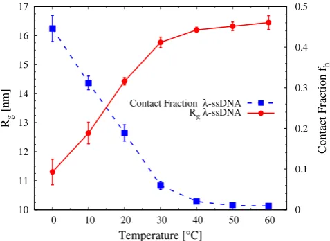
Fig. 7.Dependence of the radius of gyrationRg and the frac-tion of direct intra-chain nucleotide contacts in theλ-ssDNA sequence on the temperature.

pairing, long stems with many proximal base pairs tend to form between regions of high complementarity —these are the characteristic hairpins in fig. 8. This transition between a flexible ssDNA and significantly more rigid hairpins of dsDNA (the persistence length of dsDNA is 50 nm, around thirty times larger than that of ssDNA) is mediated by, e.g., changes in the temperature, salt con-centration or pH value. In fig. 7 we show the radius of gyrationRgand the contact fraction (the number of con-tacts Nc normalised by half the number of nucleotides in the ssDNA strand, which is the maximum number of possible base pairs) for the single-strandedλ-DNAversus temperature. A contact was defined when the

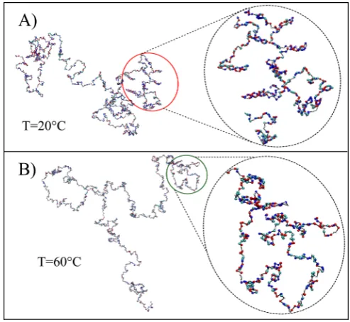
hydrogen-Fig. 8. Simulation snapshots of the λ-ssDNA sequence for three different temperatures, at 0◦C, 20◦C and 60◦C. The type of each nucleotide is represented by a colour scheme: A (white), T (cyan), G (blue) and C (red).

bonding interaction sites of any two nucleotides were less than 0.45 length units apart, regardless of the individual bases. In principle, this criterium cannot prevent stacked, nearest-neighbour nucleotides from being counted as a contact. Nevertheless it proved sufficiently accurate for a perfect dsDNA duplex where the number of contacts

Nc = N/2. Additionally, this definition will tend to in-clude mismatched base pairs in a duplex as contacts. It will thus overestimate the number of correctly-formed Watson-Crick base pairs, but for our purposes it is more important that 2Ncprovides a good estimate of the number of bases incorporated into hairpin structures.

At 0◦C, around 44% of the nucleotides are involved in contacts. When the temperature increases, the system destabilises and the number of contacts decreases signifi-cantly until it flattens out at 50◦C (the same temperature at which Rg has a plateau). However, while the contact fraction changes dramatically (more than a factor 40 from about 0.44 to 0.01) in this temperature range, there is only a small change in the radius of gyration (around a factor 1.45 from 11.3 nm to 16.4 nm). Related snapshots from simulations at selected temperatures are given in fig. 8.

We apply the same protocol as before to the pUC19 plasmid, consisting of a ssDNA sequence of 2686 nucleo-tides. For simplicity we opted for a linear molecule with freely rotating ends. The radius of gyration as a func-tion of temperature is shown in fig. 9. The behaviour is very similar to the one of λ-ssDNA, particularly the mi-nor effect that temperature changes have on Rg despite dramatic changes in the number of contacts between nu-cleotides. While for λ-ssDNA the radius of gyration at 20◦C equals 4.5% of its total contour length, in the case of the plasmidRgrepresents only 2.2%. Using the theoret-ical expression forRgin eq. (8) below and monomer length

30 35 40 45 50 55

0 10 20 30 40 50 60

0 0.1 0.2 0.3 0.4 0.5

Rg

[nm]

Contact Fraction f

h

Temperature [°C]

Contact Fraction pUC19 ssDNA R_g pUC19 ssDNA

Fig. 9.Dependence of the radius of gyrationRg and the frac-tion of direct intra-chain nucleotide contacts in the ssDNA pUC19 plasmid sequence on the temperature.

but generally consistent with the latter. At around 50◦C

Rgreaches a plateau, which is at least constant within the error bars. It is interesting to see that the λ-ssDNA ex-hibits the same tendency at the same temperature. As ref-erence we also modelled the double-stranded linear pUC19 plasmid, for which we measured values ofRgin the region of 130 nm at 20◦C and 170 nm at 60◦C, respectively, so about a factor 3 to 4 larger than the values ofRg we ob-tained for the ssDNA sequence.

In fig. 10 we can see that at 20◦C several nucleotides have hybridised, forming hairpin structures of 20–30 bp located along the plasmid. When we increase the temper-ature of the system up to 60◦C the hairpins disappear as self-hybridisation is suppressed, accounting for the sub-stantial reduction of intra-chain contacts.

The interpretation of these results is not entirely un-complicated as several interlinked mechanisms are at work that all influence the radius of gyration. When hairpins (or indeed any contact between bases) form, the hydrogen-bonding between nucleotides short-circuits all bases that are part of the hairpin, effectively shortening the contour length of the biopolymer. Hence, self-hybridisation leads to a smaller radius of gyration through a reduction of the effective contour length. Thus the smaller radius of gyra-tion at lower temperatures can be partly explained with basic polymer physics. On the other hand, the contribu-tion of hairpins to the total value ofRgis not zero, bearing in mind that even a rigid rod has a finite radius of gyra-tion. The impact of self-hybridisation is thusa priori not easily assessed. Moreover, regions cut out in this way are generally bulky, tending to swell the DNA strand relative to a shorter polymer with no base pairing. This constitutes an excluded volume effect which increases Rg. The exact number of hairpins and the degree of self-hybridisation depend ultimately on sequence of the ssDNA strand and are generally not quantifiable on the sole basis of polymer physics.

Nevertheless, some of the dependence of the radius of gyration on the number of formed base pairs can be

ra-Fig. 10.Simulation snapshots of the pUC19-ssDNA sequence for two different temperatures, at 20◦C and 60◦C. The type of each nucleotide is represented by a colour scheme: A (white), T (cyan), G (blue) and C (red).

tionalised using a simple and idealised physical polymer model. We assume that all nucleotide contacts are con-tained in well-defined hairpins. The single-stranded DNA can thus be modelled as a self-avoiding polymer with at-tached rigid, rod-like hairpins that are cut out of the con-tour length of the polymer.

At high temperature the base pairing can be neglected and the genome can be modelled as a self-avoiding walk (SAW) polymer with radius of gyration

Rg=

b √

6N ν

Kuhn, (7)

wherebis the Kuhn segment of the polymer. At salt con-ditions used in the oxDNA simulations, cNa= 0.2 M, the Kuhn segment length isb≈2 nm [36–38].ν is the scaling exponent [39] and NKuhn = N a/b the number of Kuhn segments in the polymer, witha= 0.65 nm [36, 37]. Scal-ing exponent of a SAW polymer isν = 0.588 which holds for poly-T ssDNA at physiological salt concentration [37]. Therefore, the radius of gyration is

Rg=

b √ 6

aN

b ν

(8)

with N the number of nucleotides. For the λ-ssDNA sequence and the linear pUC19 plasmid this leads to

Rg(N = 500) = 16.3 nm and Rg(N = 2686) = 43.8 nm, respectively.

gyration of the ssDNA is reduced to

Rg,ss=

b √ 6

a(N−2Nc)

b

ν

(9)

depending on the number of contacts Nc. Hairpins, how-ever, also contribute to Rg. Assuming that a hairpin is a rigid rod with length l (justifiable for hairpins shorter than about 100 nm) the radius of gyration of every hairpin isRg,h=l/

√

12. Ifk hairpins of equal length are formed, each hairpin will contribute

Rg,h=adsNc/

k√12

(10)

with the effective monomer length reduced due to helicity of double-stranded DNA ads = 0.34 nm. This conditions applies as all hairpins combined need to add up to the length along the contour that is in contact.

The total radius of gyration of an object is a sum over its subparts, where each subpart contributes its own ra-dius of gyration plus a centre-of-mass distance squared, weighted by the mass. The centre-of-mass of the total ss-DNA and hairpin system is therefore

cm=

fh

k

k

i=1

xi+

l

2nˆi (11)

withxi the (vector) position of thei-th hairpin base, i.e. the end where the hairpin is attached to the polymer. The centre-of-mass position of thei-th hairpin isxi+₂lnˆi with ˆni the unit vector specifying the orientation of the hairpin’s major axis. Note that only hairpins contribute because we chose the centre-of-mass of the ssDNA polymer as the origin of our coordinate system. The weight factor

fh= 2Nc/Nis determined by the fraction of total polymer mass contained in the hairpins. The quantityfhis equal to the contact fraction shown in figs. 7 and 9. The total radius of gyration of the ssDNA and hairpins system becomes

R2_g= (1−fh) R2g,ss+c2m

+fh

k

k

i=1

R2_g,h

+

xi+

l

2nˆi−cm

2

, (12)

where the first term on the right-hand side is the contri-bution of the ssDNA and the second term, the sum, is performed over all k hairpins. Note that the fraction of total mass in each hairpin isfh/kandxi+₂lˆni−cmis the distance between the hairpin centre of mass and single-stranded polymer centre of mass.

Assuming that the positions of hairpins are uniformly random and uncorrelated, inserting eq. (11) into eq. (12) and employing some basic algebra outlined in appendix B, the expected value for the squared radius of gyration is obtained

R2g

=R2g,ss

1−f 2 h

k

+Rg,h2

4fh−3

f2 h

k

(13)

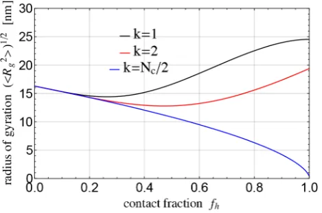
Fig. 11.Radius of gyrationpR2

gas a function of the contact fractionfh= 2Nc/Nfor different number of formed hairpinsk. The curves were obtained from eq. (13) using the following pa-rameters: Kuhn segmentb= 2 nm, nucleotide sizea= 0.65 nm, double-stranded nucleotide effective sizeads= 0.34 nm, scaling exponentν= 0.588, number of nucleotidesN= 500.

with Rg,ss and Rg,h given by eqs. (9) and (10), respec-tively, and the contact fractionfh= 2Nc/N.

We have assumed that hairpins do not interact with the ssDNA polymer, or with other hairpins, and that all

khairpins are of the same length. However, even this rel-atively simple, idealised derivation demonstrates that the radius of gyration depends on both the number of con-tacts and the hairpin length. This is shown in fig. 11 for a sequence ofN = 500 nucleotides,i.e.the length of ourλ -ssDNA. The dependence on the number of contacts is ob-viously non-monotonous. The valuesk= 1 andk=Nc/2 (assuming a hairpin needs at least 2 contacts to be la-belled as a hairpin) are the limits of the possible hairpin distribution and corresponding values forR2

gprovide the upper and lower physical limit for the expected value of the radius of gyration. The simulations, fig. 7, result in a radius of gyration around 12.6 nm and 11.3 nm at the observed contact fraction of around 32% and 45%, respec-tively, in good agreement with the theoretical prediction shown on fig. 11. We also see that for an even larger num-ber of contacts the possible range of values ofR2

gis quite wide. This is of course a much idealised and simplified reasoning, but it elucidates the non-trivial nature of these interdependencies. The theory neglects the excluded vol-ume of regions cut out of the contour length by hybridis-ation; taking this into would increase the R2

g in eq. (12), while additional bases cut out by hybridisation but not contributing to Nc would decrease it. We speculate that the two effects cancel out, to a degree, resulting in a good agreement between theory and simulations.

7 Conclusions

using the model significantly. Moreover, it allows to com-bine this coarse-grained force field with different features that are already enabled in LAMMPS.

The Langevin-type rigid-body integrators that are dis-tributed together with the LAMMPS USER-package, par-ticularly the DOT-C integrator, offer additional advan-tages over the existing standard rigid-body integrators for Langevin dynamics. They show improved stability at the costs of a very small overhead. This permits larger timesteps and therefore larger physical simulation times.

The parallel performance of the MPI-only implementa-tion, as demonstrated through scaling tests using a simple benchmark, is excellent provided there are at least a few dozen particles per MPI-task. These results show effec-tively that the oxDNA model is well suited for large and extremely large problems in DNA and RNA modelling. It can tackle problem sizes that were well beyond the reach of the original standalone implementation of the model. It is worth mentioning that the GPU-accelerated version of the standalone code is also limited to speedups of typi-cally a factor 30 compared to the single core performance. Based on the scaling analysis of the benchmarks it could be said that this is matched by the performance of a single multi- or many core chip.

The applications we opted for, a sequence of lin-ear, single-stranded λ-bacteriophage and pUC19 plas-mid DNA, are motivated primarily by currently ongoing projects in the under-investigated area of single-stranded DNA, rather than by an attempt to harvest the perfor-mance of the new LAMMPS implementation. The results shows that the conformation of ssDNA is strongly affected by the tendency to self-hybridise upon cooling,i.e.to form intra-chain base pairs between complementary nucleotides on the same strand that lead to hairpins, local regions of dsDNA, and less structured domains of clustered nu-cleotides. The radius of gyration Rg of both ssDNA ex-amples is predicted to be relatively insensitive towards temperature changes between 0◦C and 60◦C. The slight reduction of Rg can be at least partly explained with a shorter effective contour length of the biopolymer due to hairpin formation. This explanation, however, disregards some of the more subtle intricacies of the self-hybridisation process. Hairpins contribute as well to the total value of

Rg. The hybridised domains of clustered nucleotides in-troduce an excluded volume effect, which increases the radius of gyration. Last but not least, the DNA sequence determines whether any self-hybridisation can occur in the first place. It should be noted that there is a large number of possible self-hybridised bonding configurations. This means that the system is likely to fall into a particu-lar one upon quenching and to remain there. However, by using a number of independent configurations we have pre-sumably reached states that are representative, although these are not guaranteed to be the most stable ones.

In the future it may be possible to focus on ring mo-lecules that contain superhelical twist and have different number of helical turns compared to their natural form. These rings may be opened by introducing a single-strand break, which releases the superhelical twist, a mechanism

that is known to be highly relevant during gene replication and expression.

This work was funded under the embedded CSE programme of the ARCHER UK National Supercomputing Service (eCSE05-10). YAG-F acknowledges support from the Mexican National Council for Science and Technology (CONACyT, PhD Grant 384582). TC acknowledges support from the Herchel Smith Scholarship and the CAS PIFI Fellowship. TEO acknowl-edges his Royal Society University Research Fellowship. OH acknowledges support from the EPSRC Early Career Fellow-ship Scheme (EP/N019180/2).

Author contribution statement

OH, YAG-F, TC and TEO designed and performed re-search, analysed data, and wrote the paper. The imple-mentation was undertaken in a collaboration between OH and TEO.

Appendix A. Profiling

Profiling allows a detailed analysis of the implementation and gives an overview of how much time the code spends in each individual subroutine. We used the Craypat Perfor-mance Tools on the ARCHER UK National Supercomput-ing Service to conduct samplSupercomput-ing experiments of the high-and low-density benchmarks. Although the experiments where actually performed with the oxDNA model, the re-sults are representative as well for oxDNA2 as the only difference between the two is a different local geometry of the interaction sites and an additional pair interaction in form of a Debye-H¨uckel potential.

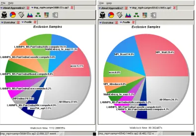
Figure 12 shows a pie chart of the low-density (LD) run. The image on the left shows the results on a single node with 24 MPI-tasks, whereas the image on the right is for 2048 MPI-tasks. Focussing first on a single node, calls to the MPI-library are below 5% and do not ap-pear with an individual pie section. The total time spent in the force calculation is around 86% (according to the LAMMPS breakdown). Interestingly, a significant fraction of the time is spent on calculating the local body coordi-nate system of the nucleotide from the quaternion degrees of freedom (MathExtra::q to exy, 11.3%).

Fig. 12.Craypat performance analysis of a sampling experiment for the low-density benchmark (60 kbp) on a single node (left, 24 MPI-tasks) and for 2048 MPI-tasks (right). Note that the assigned colour code for the functions is different in both cases.

in the first place. We decided deliberately against this possibility as this would require calculation of four force and torque components in quaternion space. The calcula-tion with 3-vectors on the other hand, as currently imple-mented, requires only three force and torque components. Perhaps most importantly, they can be made available di-rectly to the other LAMMPS routines. It is thus very likely that a performance gain from avoiding the transformation would be outweighed either by the larger number of addi-tional components and generalised quaternion forces and torques which also had to be communicated across the process boundaries or by disadvantages from a software engineering point of view.

The large fraction of the inverse cosine is more difficult to optimise. It emerges in the stacking, cross- and coax-ial stacking and hydrogen bonding interactions through a partial derivative with respect to the relative distances. A previous version of the implementation spent a whop-ping 29% of its time calculating the inverse cosine. This prohibitively large figure could be cut down to the cur-rent 12% by introducing appropriate early-rejection crite-ria in each force calculation. Further improvements might be possible through small-argument approximations of the inverse cosine. This will be tested in a future version of the code (e.g.for the upgrade to oxDNA 2.0).

At 2048 MPI-tasks, shown on the right of fig. 12, the code spends more than 50% of its time in call to the MPI-library. The percentage of time in the force calculation has fallen to about 43%. As stated above, this is primarily the consequence of an insufficient number of local atoms with

respect to the number of ghost atoms, and does not reflect a problem with the parallel performance of the implemen-tation.

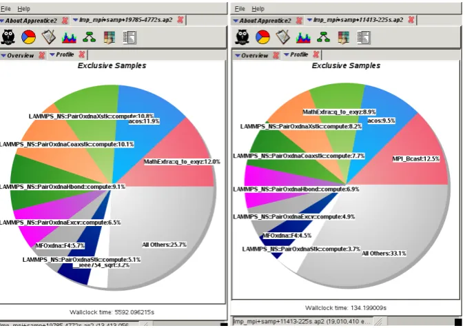
For the HD benchmark on a single node, shown on the left in fig. 13, calls to the MPI-library are below 3%. The conversion of quaternions to 3-vectors (Math-Extra::q to exyz) and the calculation of the inverse co-sine (acos) are constant at about 12%. At 2048 MPI-tasks we observe a parallel efficiency of about 85%. The time spent in the force calculation is still about 82% (accord-ing to the LAMMPS breakdown) with calls to the MPI-library amounting to just below 13%. The CPU time of the quaternion conversion to the local body frame of the nucleotide and the inverse cosine each at are around 9% due to the larger share of the calls to the MPI-library.

Appendix B. Derivation of

R

We assume that the position of hairpin bases, as well as the orientation of hairpins, is uniformly random and un-correlated along the ssDNA contour, formally: xi= 0, x2_i =R2g,ss, xixj = 0 for i =j, and similarly for the orientation: nˆi = 0, ˆn2i = 1, nˆinˆj = 0 for i = j, xiˆnj= 0. These properties result in

cm= 0

and

c2m

=f 2 h

k R

2

g,ss+l2/4

Fig. 13. Craypat performance analysis of a sampling experiment for the high-density benchmark (960 kbp) on a single node (left, 24 MPI-tasks) and for 2048 MPI-tasks (right). Note that the assigned colour code for the functions is different in both cases.

The average R2

g becomes

R2g

= (1−fh)R2g,ss+ (1−fh)

c2m

+fhR2g,h

+fh

k

i

xi+

l

2nˆi−cm

2

. (B.1)

The average of the sum is

_k

i=1

xi+

l

2nˆi−cm

2

= k

i=1

x2_i+c2_m+l 2

4

ˆ

n2_i

+lxinˆi −2xicm −lnˆicm

=

kRg,ss+fh2 R2g,ss+l2/4

+kl

2

4 −2fhR 2 g,ss−fh

l2 2

(B.2)

using that _ixicm = fkh

ijxi(xj+ 2lˆnj)= fhRg,ss2 and_inˆicm=fh₂l. Furthermore,l2= 12R2g,h.

Using these relations the expected value for the squared radius of gyration is obtained

R_g2=R2_g,ss

1−f 2 h

k

+R2_g,h

4fh−3

f2 h

k

, (B.3)

with Rg,ss and Rg,h given by eqs. (9) and (10), respec-tively, and the contact fractionfh= 2Nc/N.

Open Access This is an open access article distributed under the terms of the Creative Commons Attribution License (http://creativecommons.org/licenses/by/4.0), which permits unrestricted use, distribution, and reproduction in any medium, provided the original work is properly cited.

References

1. C. Calladine, H.R. Drew, B.F. Luisi, A.A. Travers, Un-derstanding DNA(Elsevier Academic Press, London, UK, 2004).

2. C.A. Laughton, S.A. Harris, WIREs Comput. Mol. Sci.1, 590 (2011).

3. D.A. Potoyan, A. Savelyev, G.A. Papoian, WIREs Com-put. Mol. Sci.3, 69 (2013).

4. P.D. Dans, J. Walther, H. G´omez, M. Orozco, Curr. Opin. Struct. Biol.37, 29 (2016).

5. C. Maffeo, T.T.M. Ngo, T. Ha, A. Aksimentiev, J. Chem. Theory Comput.10, 2891 (2014).

6. N. Korolev, D. Luo, A. Lyubartsev, L. Nordenski¨old, Poly-mers6, 1655 (2014).

7. M. Maciejczyk, A. Spasic, A. Liwo, H. Scheraga, J. Chem. Theory Comput.10, 5020 (2014).

8. S. Pronk, S. Pall, R. Schulz, P. Larsson, P. Bjelkmar, R. Apostolov, M.R. Shirts, J.C. Smith, P.M. Kasson, D. van der Spoelet al., Bioinformatics29, 845 (2013).

9. M.R. Machado, S. Pantano, J. Chem. Theory Comput.32, 1568 (2016).

10. J.J. Uusitalo, H.I. Ingolfsson, P. Akhshi, D.P. Tieleman, S.J. Marrink, J. Chem. Theory Comput.11, 3932 (2015). 11. J.C. Phillips, R. Braun, W. Wang, J. Gumbart, E. Tajkhorshid, E. Villa, C. Chipot, R.D. Skeel, L. Kale, K. Schulten, J. Comput. Chem.26, 1781 (2005).

12. C. Markegard, I. Fu, K. Reddy, H. Nguyen, J. Chem. Phys. B119, 1823 (2015).

13. http://lammps.sandia.gov.

14. D.M. Hinckley, G.S. Freeman, J.K. Whitmer, J.J. de Pablo, J. Chem. Phys.139, 144903 (2013).

15. D.M. Hinckley, J.J. de Pablo, J. Chem. Theory Comput. 11, 5436 (2015).

17. Y.A.G. Fosado, D. Michieletto, J. Allanet al., Soft Matter 12, 9458 (2016).

18. T.E. Ouldridge, A.A. Louis, J.P.K. Doye, J. Chem. Phys. 134, 085101 (2011).

19. T. Ouldridge, PhD Thesis, University of Oxford (2011).

20. https://dna.physics.ox.ac.uk.

21. T. Ouldridge, R. Hoare, A. Louis, J. Doye, J. Bath, A. Turberfield, ACS Nano7, 2479 (2013).

22. J. Holbrook, M. Capp, R. Saecker, M. Record, Biochem-istry38, 8409 (1999).

23. J. SantaLucia jr., D. Hicks, Annu. Rev. Biophys. Biomol. Struct.33, 415 (2004).

24. B. Snodin, F. Randisi, M. Mosayebi, P. Sulc, J. Romano, F. Romano, T. Ouldridge, R. Tsukanov, E. Nir, A. Louis

et al., J. Chem. Phys.142, 234901 (2015).

25. P. Sulc, F. Romano, T. Ouldridge, L. Rovigatti, J. Doye, A. Louis, J. Chem. Phys.137, 135101 (2012).

26. https://ccpforge.cse.rl.ac.uk/gf/project/cgdna.

27. M.P. Allen, D.J. Tildesley,Computer Simulation of Liquids

(Oxford University Press, Oxford, UK, 1989). 28. M. Allen, G. Germano, Mol. Phys.104, 3225 (2006).

29. https://www.paraview.org.

30. W. Humphrey, A. Dalke, K. Schulten, J. Mol. Graphics 14, 33 (1996).

31. R.L. Davidchack, T.E. Ouldridge, M.V. Tretyakov, J. Chem. Phys.142, 144114 (2015).

32. T.F. Miller, M. Eleftheriou, P. Pattnaik, A. Ndirango, D. Newns, J. Chem. Phys.116, 8649 (2002).

33. L. Rovigatti, F. Smallenburg, F. Romano, F. Sciortino, ACS Nano8, 3567 (2014).

34. C.D. Michele, L. Rovigatti, T. Bellinic, F. Sciortino, Soft Matter8, 8388 (2012).

35. LAMMPS Documentation, http://lammps.sandia.gov/

doc/Manual.html(2016) Chapt. 8: Performance and

Scal-ability.

36. N.M. Toan, C. Micheletti, J. Phys.: Condens. Matter 18, S269 (2006).

37. A.Y.L. Sim, J. Lipfert, D. Herschlag, S. Doniach, Phys. Rev. E86, 021901 (2012).

38. H. Chen, S.P. Meisburger, S.A. Pabit, J.L. Sutton, W.W. Webb, L. Pollack, Proc. Natl. Acad. Sci. U.S.A.109, 799 (2012).

39. P.G. de Gennes, Scaling Concepts in Polymer Physics