Mixed Tiling Systems

Mixed Tiling Systems

Alexandra Grant

May 2018

Declaration

The work in this thesis is my own except where otherwise stated.

Acknowledgements

First and foremost, I would like to thank my terrific supervisor Michael Barnsely. Thank you for giving me a taste of mathematical research and encouraging me to think independently!

I would also like to thank the many fantastic academics and lectures in the MSI whose great courses have taught me lots of interesting maths. Thanks to my fellow honours students in both the 2017 and 2018 cohorts for creating a fun and supportive study environment.

I thank my housemates and friends for keeping life full of adventures. I am also grateful for the many spectacular running trails around Canberra. Finally, I would like to thank my parents and brother for their love and support over the years.

Abstract

This thesis extends the theory of tiling iterated function systems developed in [BV18] and connects the theory to other areas of the tiling literature. The first two chapters provide background material, introduce tiling iterated function sys-tems, and discuss properties of the tilings generated from these systems. Simple examples are showcased and repeatedly referenced throughout the thesis. The third chapter links the symbolic tiling theory to Anderson and Putnam tiling theory [AP98] and the fourth chapter connects the theory to the work of Bandt on neighbour graphs [BM18]. An extension to the neighbour graph theory is proposed which allows the application of these techniques to a wider range of tiling iterated function systems. The final and title chapter of this thesis extends the symbolic tiling theory to mixed tiling systems. The notation and general framework for creating tilings from a family of tiling iterated function systems is presented. The examples considered in the mixed setting cover one-dimensional tilings, tilings with statistical circular symmetry, and tilings made from tiles with no interior. It is explained how these ideas are related to V-variable and super-fractal theory.

Contents

Acknowledgements v

Abstract vii

1 Tiling Iterated Function Systems 1

1.1 Graph Iterated Function Systems . . . 1

1.2 Attractors and Code Space . . . 4

1.3 Tilings . . . 6

1.4 Examples . . . 11

1.4.1 Fibonacci . . . 11

1.4.2 Golden-B . . . 12

2 Local Rigidity 15 2.1 Definition and Consequences . . . 15

2.2 Inflation and Deflation . . . 18

2.3 More Examples . . . 19

2.3.1 Sierpinski . . . 20

2.3.2 Rigid Williams . . . 21

3 Anderson-Putnam Theory 23 3.1 Substitution tiling systems . . . 23

3.1.1 Substitution golden-b IFS . . . 24

3.1.2 Space of Tilings . . . 26

3.2 Forces its Border . . . 28

3.3 Collared Tiles . . . 30

4 Neighbour Graphs 35 4.1 Uniform Scaling . . . 36

5 Mixed Tilings Systems 49

5.1 Notation and Set-up . . . 50

5.2 One-Dimensional Mixed Tilings . . . 55

5.2.1 Mixed Fibonacci . . . 55

5.2.2 Mixed Decorated Halves . . . 56

5.3 Fractal Pinwheel Tilings . . . 59

5.4 Mixed Sierpinski . . . 63

5.5 1-Variable Tiling IFS . . . 66

Chapter 1

Tiling Iterated Function Systems

This chapter introduces the algebraic and symbolic tiling theory developed in research by Barnsley and Vince (B & V) [BV17b, BV18]. Using the inverse maps of an iterated function systems to study tilings is well-established in the literature (see [Ban97] for example). A main contribution of B & V is presenting a simple, unifying method to construct tilings from iterated function systems that fully captures the symbolic story and easily applies to tilings of fractal blow-ups where the tiles may have no interior.

We begin, in section 1.1, by defining graph iterated function systems and introducing convenient notation. Section 1.2 reviews basic fractal theory on at-tractors and code space. These two sections prepare the reader for section 1.3 which defines and discusses tiling iterated function systems. Finally, section 1.4 showcases two key examples.

The notation, definitions and theorems in this chapter mostly follow [BV18]. The other chapters of this thesis use the language introduced here and build on this symbolic framework. In particular, chapter 2 focuses on tiling iterated function systems that satisfy a property known as ‘local rigidity’.

1.1

Graph Iterated Function Systems

A hyperbolic iterated function system (IFS) consists of a complete metric space together with a finite set of strictly contractive maps. Since all the IFSs we con-sider are hyperbolic, we refer to them simply as IFSs for the remainder of this thesis. It is well-known that these systems can be used to create self-similar frac-tals (see [Hut81] for example). Also known, but maybe less widely appreciated, is that ‘quasiperiodic’ (defined in section 1.3) tilings can be constructed as fractal

blow-ups of certain IFSs. We concern ourselves with the generalisation of these ideas to the graph (directed) IFS setting [BV18].

Definition 1.1. Let F = {f1, f2, ...fN} be a finite set of invertible contraction

maps fi : RM → RM with contraction factors 0 < λi < 1 for i ∈ {1, ...N}. Let

G = (E,V) be a finite strongly connected directed graph with edges

E ={e1, e2, ...e|E|} with E =|E|=N

and vertices V ={v1, ...v|V|} with V =|V| ≤N. The graph G provides the order in which the functions F may be composed from left to right. We call (F,G) a graph IFS. In general, we denote the edges in G by the indices {1,2, . . . N} and the vertices by elements of the set {1,2, . . . V}.

The graph G being strongly connected means there is a directed path from any vertex of the graph to any other vertex. We introduce a supply of convenient notation for various sets of vertices and edges in G.

Notation 1.2. Define

- Ev,w as the set of directed edges in G from vertex w to vertexv,

- Ev,∗ :={u∈ Ev,w : w∈ V} as the set of directed edges with the final vertex

specified,

- E∗,v := {u ∈ Ew,v : w ∈ V} as the set of directed edges with the initial

vertex specified,

- Σ0 as the empty string ∅,

- Σk as the set of directed paths in G of length k∈N,

- Σ∗ :=∪k∈N0Σk as the set of directed paths of finite length,

- Σ∞ as the set of directed paths of infinite length, and - Σ := Σ∗∪Σ∞.

So Σ is the set of finite and infinite paths in G that by Definition 1.1 corre-sponds to the allowed compositions of functions fromF . The sequence of directed edges (eσ1, eσ2, . . . eσk) corresponds with the composition fσ1 ◦fσ2 ◦. . .◦fσk.

1.1. GRAPH ITERATED FUNCTION SYSTEMS 3

the definitions in Notation 1.2, let Σ†₀ be the empty string ∅, Σ†_k be the set of directed paths in G† _{of length k ∈}

N, and Σ†∞ be the set of directed paths of infinite length. Define

Σ†:= Σ†_∗∪Σ†_∞ where Σ†_∗ :=∪k∈N0Σ

†

k.

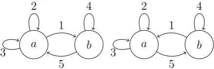
Example 1.3. To give the reader something concrete to follow, we introduce an example graph IFS . Let F = {f1, ..., f5} be a set of five contractive maps

with scaling factor 0 < s < 1. We do not define explicit maps here but note that the Penrose IFS takes this form. The allowed composition of functions in

F is determined by the graph G displayed at the left of Figure 1.1. On the right side of the same figure, we display the reverse graph G†_{. The vertex set for} both of these graphs is V = {a, b}. The strings 145314 and 125413 correspond to example directed paths of finite length in G and G† _{respectively. So by the} notation introduced above, 145314∈Σ∗ and 125413∈Σ†_∗. We emphasise that Σ and Σ† are subspaces of the code space (see Remark 1.4) that contains all finite and infinite strings made from elements in the set [5] ={1,2,3,4,5}.

a b a b

1 2

3

5 4

5 2

3

1 4

Figure 1.1: Penrose IFS graph G and reverse graph G†

Remark 1.4. The structure of code spaces is thoroughly discussed in the fractals literature (see [Bar93] and [Bar06] for example) Set [N] := {1,2,· · ·N}, then define [N]k_{as the set of strings of lengthk, [N]}∗_{as the set of strings of finite length} and [N]∞ as the set of strings of infinite length. The space [N]∗∪[N]∞ is a code space and can easily be equipped with a metric d[N]∗_∪[N]∞ such that it becomes a

compact metric space [BV17b]. With an induced subspace metric dΣ, the space

Σ, defined for a graph IFS withN maps, is a shift invariant compact subspace of [N]∗∪[N]∞. For the shift transformation S : [N]∗ ∪[N]∞ →[N]∗∪[N]∞ which removes the first element of the string, we have that S|Σ : Σ→Σ is continuous.

Notation 1.5. For θ=θ1θ2. . . θk ∈Σ∗,

fθ :=fθ1fθ2. . . fθk

f−θ :=fθ−11f

−1

θ2 . . . f

−1

θk = (fθkfθk−1. . . fθ1)

−1_.

If θ = ∅, fθ and f−θ are the identity function. For θ ∈ Σ∞ and k ∈ N0 let θ|k :=θ1θ2. . . θk. For θ ∈Σ, define the length of θ as

|θ|:=

 



k θ ∈Σk

∞ θ ∈Σ∞.

1.2

Attractors and Code Space

Before explaining how to construct tilings from a graph IFS, we review some standard fractal theory on attractors and code space. Let _H be the non-empty compact subsets of _RM. Equipped with the Hausdorff metric, the space _H is complete (see [Bar93, Theorem 7.1] for a proof). Let _HV be the product of V

copies of _H.

Definition 1.6. Define F:_HV →_HV _by

(FX)_v :={x∈feXw : e∈ Ew,v, w ∈ V} (1.1)

for all X ∈_HV_{, whereX}

w is the wth component of X.

Theorem 1.7. The map F: _HV _→

HV is a contraction. There exists a unique

vector of compact sets A= (A1, A2, ...AV)∈HV such that

A=FA and A= lim

k→∞F

k_B

for all B∈_HV_{, where convergence is with respect to the Hausdorff metric on}

HV.

Theorem 1.7 summarises the existence of a unique vector of compact sets that is the fixed point of Equation 1.1. This result is well-known in the IFS literature (for example see [MW88, Theorem 1] or [Bar93, Chapter 10]).

Definition 1.8. Define the union of the components ofAasA:=S

v∈VAv. The

set A ∈ _H is called the attractor of the graph IFS and {Av : v ∈ V} are its

1.2. ATTRACTORS AND CODE SPACE 5

For our purposes, we will always assume that the attractor components do not overlap: Ai ∩Aj = ∅ for i 6= j. If this was not the case, we could apply a

change of coordinates to make a new graph IFS that did satisfy this condition [BV18].

Example 1.9. We sketch how to obtain the attractor of an IFS with the form presented in Example 1.3. Following Definition 1.6, for any X ∈_H2

(FX)a ={x∈feXw : e∈ Ew,a, w ∈ V}

={x∈feXw : e∈ {1,2,3}}

={x∈f1Xb, x∈f2Xa, x∈f3Xa,}

(FX)b ={x∈f4Xb, x∈f5Xa}.

By Theorem 1.7, we know there exists (A, B)∈_H2_{, the unique vector of compact}

sets, with

A=f1(B)∪f2(A)∪f3(A) and B =f4(B)∪f5(A).

Ensuring that the maps were defined such that A and B do not overlap, we call

P :=A∪B the attractor of the IFS. Figure 1.2 displays this construction for the Penrose IFS whose maps have scaling factor 1_τ whereτ = 1+

√

5

2 is the golden ratio

(for explicit maps see [BV14]).

Figure 1.2: Penrose IFS attractor

Definition 1.10. Define −→v (i),←−v(i) ∈ V as the unique vertices such that ei is

the directed edge in G from←−v(i) to −→v(i) .

Definition 1.11. The coding map π : Σ→_H(A) is defined by

π(_∅) =A,

π(ω) =fω(A−→v(ωk)) for all ω=ω1ω2. . . ωk∈Σ∗, k ∈N

π(σ) = lim

where the limit is with respect to the Hausdorff metric and_H(A) is the non-empty compact subsets of A.

Theorem 1.12. The coding map π : Σ → _H(A) is well-defined and

continu-ous with respect to the Hausdorff metric. When restricted to Σ∞, the map π is

continuous from Σ∞ to _RM _and

π(Σ∞) = {π(σ) :σ ∈Σ∞}=∪v∈VAv =A

The coding map provides an address space structure for the attractor. For a thorough explanation of the relationship between subsets of the attractor and address spaces from this perspective see [Bar06, Chapter 3].

1.3

Tilings

Everything we have introduced so far holds for all graph IFSs. To define a tiling IFS extra conditions are required.

Definition 1.13. Let F = {_RM_;f

1, f2· · ·fN} with N ≥ 2 and graph G be a

graph IFS of contractive similitudes where for fixed 0 < s <1 the scaling factor of each fi is λi =sai with ai ∈N. Also suppose gcd{a1, a2, ...aN}= 1 and define

amax= max{ai :i= 1,2, ...N}.

For x∈_RM_{, the function f}

i :RM →RM is defined by

fi(x) =saiOi(x) +qi

whereOi is an orthogonal linear transformation andqi ∈RM. Let DH(X) be the

Hausdorff dimension of X ⊂_RM_{. It is required that}

DH(fe(A−→v(e))∩fl(A−→v(l)))< DH(A)

for all e, l ∈ E with e 6= l. Also ensure that Ai ∩Aj = ∅ for all i 6= j. If these

conditions are satisfied then (F,G) is called a tiling IFS.

1.3. TILINGS 7

components must be smaller than the Hausdorff dimension of the attractor. For an thorough explanation of Hausdorff dimensions see [Hut81].

When investigating a fractal generated from an iterated function system, one often starts with the attractor and zooms in to see similar copies of the attractor on smaller scales. Instead of zooming in, the construction of tilings is motivated by expanding outwards. The idea is to take the attractor and expand and split it appropriately so that the new larger set is made from scaled copies of the original attractor. This explains why tilings made in this way are often referred to as ‘fractal blow-ups’. The scaled copies, associated with strings of maps, are the fractal tiles in the tiling. To make sure the tiles are appropriately sized, we need to keep track of the scaling factors of the maps. Since the maps in a tiling IFS have scaling factors that are integer powers of some fixed 0< s < 1, we define ξ

and ξ− as functions on code space whose values are the sum of elements in the set{a1, a2, ...aN}.

Definition 1.14. For σ=σ1σ2...σk∈Σ∗, define

ξ(σ) = aσ1 +aσ2 +...+aσk

ξ−(σ) = aσ1 +aσ2 +...+aσk−1

and ξ(∅) =ξ−(∅) = 0. We call ξ(σ) the scaling length of σ.

Next, we define sets of strings that start at a specified vertex in the graph and whose scaling length are only just larger than some fixed positive integer value. A key idea captured in a forthcoming proposition is that the elements in this set are in bijective correspondence with tiles in some bounded tilings.

Definition 1.15. For all k ∈_N0 and v ∈ V, define scaling sets as

Ωv_k={σ∈Σ∗ :ξ(σ)> k≥ξ−(σ), σ1 ∈ E∗,v},

Ωk=

[

v∈V

Ωv_k ={σ∈Σ∗ :ξ(σ)> k≥ξ−(σ)}.

Using these scaling sets, the tiling map Π is defined from directed paths in the reverse graph G† _{to the collection of compact subsets of}

H(RM) as follows.

Definition 1.16. The tiling map Π : Σ†→_H(_H(_RM_{)) is}

Π(θ1θ2...θk) :={f−θ1θ2...θkπ(σ) :σ ∈Ω

v

for θ ∈Σ†_∗, where v is the unique vertex such that θk is a directed edge in G† to

vertex v, and

Π(θ) := [

k∈N

Π(θ|k).

for θ ∈Σ†_∞.

For convenience, let_T∗ := Π(Σ†∗) andT∞ := Π(Σ†∞) be the set of tilings made from strings of finite and infinite length respectively. Let _T := Π(Σ†) be the union of these sets.

Definition 1.17. The prototile set P of a tiling T is a minimal set of tiles such that every tile in T is an isometric copy of a tile in P.

Remark 1.18. The image of the tiling map is contained in the space_H(_H(_RM)), the space of compact subsets of the sets of compact subsets of the metric space (_RM, d) with d the usual Euclidean metric. Thinking of a tiling as a set of tiles, each of which is a compact subset of _RM, it is clear that tilings are points in

H(H(RM)).

In [BV18] the authors describe a convenient metric for tiling spaces. Let U

denote the group of isometries of_RM _{and fixT some group contained inU. Also,}

fix a prototile set P. Define _T0 as the set of all tilings on _RM _{made from tiles}

in P mapped by elements of T. Let t∅ be the empty tile which can be thought of as a tile at infinity. The usual M-dimensional stereographic projection to the

M-sphere is denoted ρ:_RM _→

SM. Define ˆρ:T0 →SM by

ˆ

ρ(T) ={ρ(t) : t∈T, t6=t∅} ∪ρˆ(t∅)

where ˆρ(t∅) takest∅to the top of the sphere diametric to the origin. LetH(H(SM))

be the nonempty compact subsets of the nonempty compact subsets of _SM. By [Bar06, Chapter 1], (_H(_H(_SM)), d_H(H(SM))) is a compact metric space. Then the tiling metric on _T0 is defined as

d_T0(T₁, T₂) = d

H(H(SM))( ˆρ(T1),ρˆ(T2)). The space (_T0, d_T0) is compact [BV18].

Definition 1.19. A tiling T is quasiperiodic (also called repetitive in the litera-ture) if for any patch P in T there exists a RP >0 such that any ball of radius

RP contains an isometric copy of P. Two tilings are locally isomorphic if any

1.3. TILINGS 9

Definition 1.20. A symmetry of a tiling is an isometry that takes tiles to tiles. A tiling is periodic if there exists a translational symmetry. In other terms, a tilingT, a subset of_RM_{, is periodic ifT =T+v for somev ∈}

RM. If no non-zero

vector v ∈_RM _{exists, the tiling is called non-periodic.}

Definition 1.21. An IFS (F,G) is purely self-referential if Ev,v 6=∅ for allv ∈ V.

The following theorem, stating properties of tilings in the set _T, is presented in [BV18, Theorem 4 and Theorem 6], generalising the results and proofs from [BV17b]. In later sections and chapters we refer to various parts of this theorem as it relates to examples and other results.

Theorem 1.22. Let (F,G) be a tiling IFS.

(a) Each set Π(θ) in _T is a tiling of a subset of _RM_{, the subset being bounded}

when θ∈Σ†_∗ and unbounded when θ ∈Σ†_∞.

(b) For all θ∈Σ†_∞, the sequence of tilings {Π(θ|k)}∞

k=1 is nested according to

Π(θ|1)⊂Π(θ|2)⊂Π(θ|3)...

(c) If (F,G) is purely self-referential, then for all θ ∈ Σ†, with |θ| sufficiently large, the prototile set for Π(θ) is

P ={si_A

v :i∈ {1,2, ...amax}, v ∈ V}. (d) The map

Π : Σ† →_T⊂_T0

is continuous from the compact metric space(Σ†, d_Σ†)into the compact

met-ric space (_T0, d_T0).

(e) Each tiling in _T∞ is quasiperiodic and each pair of tilings in T∞ are locally

isometric.

Definition 1.23. The sequence of tilings

Tk :=s−kπ(Ωk) and Tkv :=s

−k_π(Ωv k)

for k ∈_N and v ∈ V are called the canonical tilings of the tiling IFS (F,G). Theorem 1.24. For all θ∈Σ†_∗,

Π(θ) =EθT

− →_v(θ

|θ|)

ξ(θ) ,

for Eθ =f−θsξ(θ).

Proof. Writing θ=θ1. . . θk with |θ|=k, it follows that

Π(θ) = f−θ1...θk{π(σ) :σ ∈Ω

− →_v(θ

k)

ξ(θ1...θk)}

=f−θ1...θks

ξ(θ1...θk)_s−ξ(θ1...θk)_{{π(σ) :σ ∈Ω}

− →_v(θ

k)

ξ(θ1...θk)}

=Eθ1...θkT

− →_v(θ

k)

ξ(θ1...θk).

Every bounded tiling is related by isometry to some canonical tiling. We refer back to proof of Theorem 1.24 explicitly in section 5.1 with regards to a similar result in the mixed tiling setting.

Definition 1.25. The relative address of a tile t∈T_kv is defined as ∅.π−1_sk_(t)∈

∅.Ωv_k.

Relative addresses put an address space structure on the set of canonical tilings. The next proposition follows directly from the definition ofTkand relative

addresses since the map s−kπ: Ωk →Tk is surjective and injective.

Proposition 1.26. The tiles of Tk are in bijective correspondence with the set of

relative addresses ∅.Ωk.

By Theorem 1.24 every tiling of the form Π(θ) for some θ ∈ Σ is related by isometry to the canonical tilingTξ(θ). Then from Proposition 1.26, it is clear that

1.4. EXAMPLES 11

1.4

Examples

The two example IFSs showcased in this section are the Fibonacci and golden-b. These two systems play a major role in our story since they are among the simplest one and two dimensional examples whose maps have more than a single scaling ratio.

1.4.1

Fibonacci

Let F ={f1 = sx, f2(x) = s2x+s : s+s2 = 1, s > 0} and G is a single vertex

graph with two loops labelled 1 and 2. We call (F,G) the Fibonacci IFS. The address space is [2]∗for finite strings and [2]∞ for infinite strings. Denote the unit interval by I. Sincef1(I)∪f2(I) = I, the attractor ofF isI. The prototile set is {a, b}wherea:=sI andb :=s2I. We callaa large tile andb a small tile. Tiling blow-ups of the form Π(θ) for θ ∈ [2]∗ look like decorations of intervals on the real line. Using Definition 1.16 we explicitly construct some example bounded tilings. The attractor is tiled by the two tiles in the set Π(∅) = {f1(I), f2(I)}

as illustrated in Figure 1.3. Next, consider Π(1) = {f−1π(θ) : θ ∈ Ω1} where

Ω1 ={11,12,2}. So

Π(1) ={f−1f11(I), f−1f12(I), f−1f2(I)}

is a bounded tiling made from three tiles pictured at the top of Figure 1.4. The relative addresses, identified from the set Ω1 are labelled under each tiling. Since

Figure 1.3: Fibonacci tiling Π(∅)

ξ(2) > ξ(1) we expect the bounded tiling Π(2) to have more tiles than Π(1). Observe that Π(2) ={f−2π(θ) :θ ∈Ω2} where Ω2 ={111,112,12,21,22} so

Π(2) = {f−2f111(I), f−2f112(I), f−2f12(I), f−2f21(I), f−2f22(I)}

pictured at the bottom left of Figure 1.4.

The tiling Π(11) is pictured to the right of Π(2) for comparison. Since ξ(2) =

Figure 1.4: Fibonacci tilings Π(1), Π(2) and Π(11)

to the right. Determining when two tilings are translations, or more generally isometries of one another, is a key idea explored in section 2.1.

Often for convenience, we write canonical Fibonacci tilings as strings of the form

T0 =ab T1 =aba T2 =abaab T3 =abaababa T4 =abaababaabaab

where a is the big tile and b is the small tile.

Figure 1.5: Golden-b attractor

1.4.2

Golden-B

Just like the Fibonacci IFS, the golden-b IFS has two maps F = {f1, f2} with

1.4. EXAMPLES 13

are

f1 x y

!

= 0 s

−s 0

!

x y

!

+ 0

s

!

and f2 x y

!

= −s

2 ₀

0 s2

!

x y

!

+ 1

0

!

.

The attractor is the hexagon G ∈ _R2 _{which is the only rectilinear polygon that}

can be tiled by two different scaled copies of itself [BV17b]. We defineL:=f1(G)

the large tile and S := f2(G) the small tile (see Figure 1.5). The golden-b IFS

has an identical addresses space to the Fibonacci IFS: [2]∗ for finite strings and [2]∞ for infinite strings. Figure 1.6 shows the bounded tilings Π(1),Π(2) and Π(11). Figure 1.7 depicts the first 4 canonical tilings with their relative addresses labelled.

Figure 1.6: Golden-b Π(1),Π(2) and Π(11) tilings [BV17b]

Chapter 2

Local Rigidity

This chapter explains some consequences when a tiling IFS is ‘locally rigid’. Im-portantly, when a tiling IFS satisfies this condition it admits an invertible inflation map. The existence of an invertible inflation map is a key requirement for the tiling systems considered by Anderson and Putnam [AP98]. We explore how the symbolic tiling theory connects to the Anderson and Putnam theory in chapter 3.

In this chapter, we primarily follow [BV18] and remain in the symbolic tiling realm, examining tilings in the image of the tiling map Π. In section 2.1 we define ‘local rigidity’ and showcase some neat consequences for the canonical sequence of tilings and tilings in the set _T. Section 2.2 describes how to construct an invertible inflation map. Finally, in section 2.3 we present two more example tiling IFSs whose tilings are made from tiles with no interiors.

2.1

Definition and Consequences

Definition 2.1. Suppose (F,G) is a graph IFS. LetT be the group of isometries generated by the set of maps in F and U be the group of all isometries on _RM_.

LetT0 _{⊂ T be the groupoid of isometries of the form f}

−θfσ whereσ ∈Σ∗,θ ∈Σ†∗ and ←−v(σ1) = −→v(θ|θ|). For θ∈Σ∗, we define the isometry Eθ :=f−θsξ(θ).

Definition 2.2. The tiling IFS (F,G) is called locally rigid when the following two conditions hold:

(i) If E ∈ T0_{, v ∈ V with T}v

0 ∩ET0v 6=∅ then E =id.

(ii) IfE ∈ T such thatTv

0 ∩ET0w tiles Av∩EAw for somev, w∈ V thenE =id

and v =w.

Theorem 2.3. If F ={fn : n ∈ [N]} has non-isometric tiles, then it is locally

rigid.

Proof. Since |V| = 1 we only need to check condition (i) from Definition 2.2.

Suppose for some E ∈ T0_{, we have T}

0 ∩ET0 6= ∅. Because the tiles are

non-isometric, there must exist n ∈[N] such that fn(A) =Efn(A). SinceE =f−θfω

for some θ, ω ∈ [N]∗, we have that fθfn(A) = fωfn(A). Hence, θn = ωn and so

θ =ω. It follows that E =f−θfθ =id.

Example 2.4. Since the golden-b and Fibonacci attractors are tiled by two non-isometric tiles, it follows as a corollary from Theorem 2.3 that they are both locally rigid. We can also see that the golden-b and Fibonacci are locally rigid IFSs by inspecting the images of their corresponding attractors (Figures 1.5 and 1.3). By trying to rotate and flip the golden-b attractor in various ways, it becomes clear that there is no isometry that maps one tile in T0 to itself that

does not also map the other tile to itself. For the Fibonacci IFS, the only way for an isometry to make a non-trivial tileable intersection of two copies of T0 would

be if it involved a reflection. However, this is not possible since the group T0 _for the Fibonacci IFS is contained within the group of translations.

Definition 2.5. Recall that for anyσ ∈Σ∗ the scaling length of σ is defined as

ξ(σ). For k ∈_N and v ∈ V, we define a subset of the scaling set as Λv_k ={σ ∈Σ∗ :ξ(σ) = k,←−v(σ1) = v} ⊂Ωvk−1,

which contains all strings with scaling length k starting at vertex v.

Supposing the IFS is locally rigid, there is a nice relationship between the copies of Tv

0 in some larger canonical tilingTkand strings in the set Λvk. We state

without proof this correspondence in the proposition below (see [BV18, Theorem 8]).

Proposition 2.6. SupposeF is locally rigid. There is a bijective correspondence between Λv

k and the set of copies ET0v ⊂Tk with E ∈ T.

Example 2.7. We consider this correspondence using the golden-b IFS. Recall from section 1.4.2 that the golden-b IFS has address space [2]∗ ∪[2]∞. So the corresponding set for scaling length 3 is

2.1. DEFINITION AND CONSEQUENCES 17

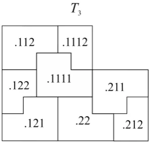
Figure 2.1 shows that there are three copies of T0 inT3 (as expected from

Propo-sition 2.6) with relative address pairs {(.1111, .1112),(.121, .122),(.211, .212)}. Moreover, from Theorem 1.24 we know there exists exactly three bounded tilings in the image of the tiling map Π that are related by isometry to T3. Since the

attractor Π(∅) must be nested in Π(θ) for any θ ∈ [2]∗, the three strings in Λ3

correspond to the possible placement of the attractor at the origin. Figure 2.2 compares the placement of Π(∅) in the bounded tilings Π(111), Π(12) and Π(21).

Figure 2.1: Golden-b T3 canonical tiling

Figure 2.2: Nesting of Π(∅) in Π(111), Π(12) and Π(21)

Theorem 2.8. Let (F,G) be locally rigid. For some θ, ψ ∈ Σ† and E ∈ T,

Π(θ) =EΠ(ψ) if and only if ∃p, q ∈_N0 such that ξ(θ|p) =ξ(ψ|q), E =Eθ|pE_ψ−|1q,

Theorem 2.8 is the core result in [BV18] showing that when an IFS is locally rigid it is possible to determine exactly when two tilings (bounded or unbounded) are related by an isometry in T. The proof of the theorem uses Proposition 2.6 and related results (see [BV18, Theorem 9]).

Corollary 2.9. If (F,G) is locally rigid, then Π(θ) = EΠ(θ) for E ∈ T if and only if E =id.

Corollary 2.9 shows that tilings generated from a locally rigid IFS have a similar property to being non-periodic. Instead of requiring that no translation vector maps the tiling to itself, the corollary shows that tilings in the image of Π have the property that no isometry from the group T maps the tiling to itself. It turns out that many locally rigid IFSs do generated tilings that are non-periodic in the translational sense (discussed in section 3.1).

2.2

Inflation and Deflation

This section explains how a locally rigid IFS admits a well-defined invertible inflation map.

Definition 2.10. Define _Q := {ET : E ∈ T, T ∈ _T} and _Q0 := {ET : E ∈ T, T ∈_T, T 6=T₀v for any v ∈ V}.

Definition 2.11. A bounded tiling P ∈ _Q is called a partner if P = ETv

0 for

some E ∈ T, v ∈ V. For Q ∈ _Q, define QP to be the set of all partners in Q.

A tile that is isometric to sAv for some v ∈ V is called a large tile. For Q∈ Q,

define QL to be the set of large tiles Q.

Definition 2.12. The amalgamation and shrink operationα:_Q0 →_Qis defined by

αQ0 ={st:t∈Q0\Q_P0 } ∪G{sEAv :E ∈ T, ET0v ⊂Q

0

P, v ∈ V}.

The expansion and splitting operation α−1 _:

Q→Q is defined by

α−1Q={s−1t:t /∈QL} ∪

G

{sET₀v :E ∈ T, sEAv ∈Q, v ∈ V}.

2.3. MORE EXAMPLES 19

Observe that_Q0 is defined as a subset of_Qwithout tilings isometric to canon-ical tilings Tv

0 for some v ∈ V. For tilings isometric to something of the form T0v,

an amalgamation and shrinking process would map outside the set _Q. This is a small technical point explaining why the map α has domain _Q0.

Proposition 2.13. If (F,G)is locally rigid, then α and α−1 are well-defined. In particular, αTk =Tk−1 and α−1Tk−1 =Tk for all k∈N.

The key idea for Proposition 2.13 (see [BV18, Theorem 10]) is that if the IFS is locally rigid we can unambiguously identify partner sets so that the operations

α and α−1 _{are well-defined. Consider the partial golden-b tiling in Figure 2.1. It}

is unambiguous how to match a small tile to a big tile. Note that in both the golden-b and Fibonacci examples only big tiles can exist without partners.

Proposition 2.14. Suppose(F,G) is locally rigid, then for all θ ∈Σ†_∞, n ∈[N],

αaθ1E−1

θ1 Π(θ) = Π(Sθ) and Enα

−an_{Π(θ) = Π(nθ).}

Proposition 2.14 (see [BV18, Theorem 11]) captures the conjugacy relation between the operations α and α−1_{, together with an isometry action, on tilings}

and the shift and adjoin operations on code space. So applying the shift opera-tion to remove the first element of the string corresponds to applying an isometry and then amalgamating and shrinking (a number of times) the tiling. In con-trast, adding an element to the front of the string corresponds to expanding and subdividing (a number of times) and then applying an isometry to the tiling.

On canonical tilings,αandα−1 _{serve as an appropriate inflation and deflation}

pair. For tilings Π(θ) withθ ∈Σ†, if we want the inflation and deflation operations to keep the tiling in the image of Π, Proposition 2.14 gives us the appropriate constructions.

2.3

More Examples

Figure 2.3: Sierpinski attractor

2.3.1

Sierpinski

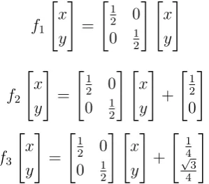
Let F ={f1, f2, f3} be the Sierpinski IFS with maps

f1 " x y # = " 1 2 0

0 1₂

# " x y # f2 " x y # = " 1 2 0

0 1₂

# " x y # + " 1 2 0 # f3 " x y # = " 1 2 0

0 1₂

# " x y # + " 1 4 √ 3 4 # .

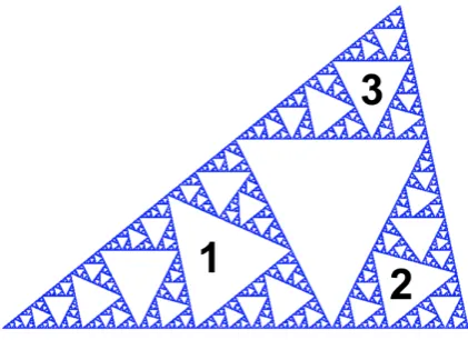
The attractor A is the Sierpinski triangle displayed in Figure 2.3. It is clear that

T0 ∩ET0 tiles A ∩EA for any E = fifj−1 with i 6= j. Figure 2.4 shows this

for the case when i = 2 and j = 1 with the tileable intersection shaded red. In a Sierpinski blow-up, it is impossible to uniquely identify partners. All the unbounded tilings are periodic, in contrast to the tilings in the next example.

2.3. MORE EXAMPLES 21

2.3.2

Rigid Williams

In their recent paper [SW18], Steemson and Williams describe the family of generalised Sierpinksi triangles which consists of four types: 4N N N, 4F N N,

4F F N,4F F F. The names of the types indicate the orientation, flip or non-flip, of the three maps in the IFS. For example, the Sierpinski IFS from section 2.3.1 has type 4N N N. The 4F F F is the well-known pedal triangle (see [ZHWD08] for example). Steemson and Williams give the first detailed description of the two other members: 4F N N (the Steemson) and4F F N (the Williams). Assuming one of the sides has length 1, a general Williams triangle has the form displayed in Figure 2.5.

Figure 2.5: General Williams fractal triangle [SW18]

The rigid Williams IFS has scaling factors α =s and β = γ = s2. The side lengths of the rigid Williams attractor must satisfy the equations:

sb+s2a= 1

s+s2b=b s2+s2a=a

Solving we finda = ₁₋s2_s2,b =

s

1−s2 and 2s2+s4 = 1. Thens=

p√

2−1≈0.644,

a ≈ 0.707, b ≈ 1.10. The explicit maps f1, f2, f3 for the IFS can be computed

Figure 2.6: Rigid Williams attractor

Under any isometry in T, the tiles can appear in one of six orientations of the attractor. These six possible orientations, three non-flip and three flip, are displayed in Figure 2.7. The idea is that we cannot intersect any of these fractal triangles so that their intersection is non-trivial and tileable. Hence, the IFS is locally rigid. For any tiling blow-up generated from the map Π : [3]∗∪[3]∞→_T, we can unambiguously identify partners and apply an amalgamation and shrink operation.

Chapter 3

Anderson-Putnam Theory

This chapter links the fractal tiling theory outlined in the previous two chapters to mainstream tiling literature. A keystone paper in the tiling literature is by Anderson and Putnam (A & P) which shows how to describe a substitution tiling space in terms of an inverse limit space [AP98]. In section 3.1, we introduce the substitution tiling systems considered by A & P and prove that it is possible to interpret these systems in the tiling IFS framework. However, we emphasise that the tiling IFS theory is more general and not restricted to tiles being homeomor-phic to disks or the action being solely contained within the group of translations. The advantage of introducing the A & P tiling perspective is that it has been thoroughly developed and widely applied to compute many things such as the cohomology of tiling spaces. In sections 3.2 and 3.3 we explain the A & P inverse limit construction and use this theory to present the well-known computations of the golden-b and Fibonacci cohomology groups.

3.1

Substitution tiling systems

We introduce substitution tiling systems in the style of [AP98] but slightly change notation and terminology to align with other material in this thesis. To A & P a tile is a subset of _RM _{that is homeomorphic to a closed ball in}

RM. A

partial tiling is a collection of tiles in _RM _{with pairwise disjoint interiors and its}

support is the union of its tiles. A tiling is a partial tiling with support_RM_{. Let}

P = {pi : i ∈ {1· · ·n}} be a finite prototile set. Let ˆ∆ be the collection of all

partial tilings that only contain translations of these prototiles. Assume there exists an inflation constant λ >1 and a substitution rule that associates to each prototilepi a partial tiling Pi with supportpi such thatλPi is in ˆ∆. The inflation

map ˆω : ˆ∆→∆ is defined byˆ ˆ

ω(T) =λ [

pi+u∈T

(Pi+u).

Let ∆ be the collection of tilings in ˆ∆ such that for any patch P ⊆ T with bounded support, P ⊆ ωˆn_({p

i +u}) for some n ∈ N, prototile pi and vector

u ∈ _RM_{. Let ω = ˆω|}

∆, then the pair (∆, ω) is the space of tilings and inflation

map studied by A & P.

Proposition 3.1. Any A & P tiling system (∆, ω) can be expressed as a tiling IFS.

Proof. Suppose (∆, ω) is an A & P tiling system with prototile set P ={pi : i∈

{1· · ·n}} and inflation constant λ > 1. We define a graph IFS (F,G) such that the number of vertices inGis the same as the number of prototiles: V =|V|=|P|. Denote the vertices V ={v1,· · ·vn}. We know that each prototilepi is associated

with a partial tiling Pi. The tiles in this partial tiling correspond to contractive

maps in F that take various attractor components of the IFS to the attractor component corresponding to the vertex i inG. That is

Avi ={x∈feAw : e∈ Ew,vi, w ∈ V}.

The set of maps constructed in this way for the partial tilings of all prototiles, together with a directed graph that describes which maps take which prototiles into which, fully defines (F,G).

It is not true that every tiling IFS can be expressed as an A & P tiling system. Firstly, the tiles in a tiling IFS are not necessarily homeomorphic to disks as we observed with the Sierpinski and rigid Williams tilings in sections 2.3.1 and 2.3.2. Even if the tiles are homeomorphic to disks, it is not always possible to create a finite prototile set such that every tile is a translation of some prototile. A well-known example is the pinwheel tiling [CR98] and in section 5.3 we discuss a new interesting example from [BMT18]. However, in many cases we can expand the prototile set of a tiling IFS to create a new tiling IFS that does fit the A & P setting. We show that this is possible for the golden-b IFS.

3.1.1

Substitution golden-b IFS

In section 1.4.2, we defined the golden-b IFS by F ={f1, f2} and let {S, L} be

3.1. SUBSTITUTION TILING SYSTEMS 25

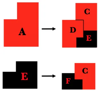
by the set of isometries that map the prototile set to the tiles in_T. By considering compositions of these isometries, we observe that in any tiling there are exactly four possible orientations for S and four orientations for L. Any tile in any tiling in _T is up to translation one of the tiles in the set {A, B, C, D, E, F, G, H}

displayed in Figure 3.1.

Figure 3.1: Substitution golden-b prototile set

We build a second golden-b IFS whose prototile set is the set of these eight tiles. An appropriate inflation map is constructed by applying α−1 _{twice so that}

the new large and small tiles in the subdivision have appropriate orientations. By expanding and splitting twice, the small tiles are subdivided into one small and one large tile, while the large tiles are subdivided into one small and two large tiles. Figure 3.2 shows the subdivision for prototiles A and E.

Figure 3.2: Subdivision for prototiles A and E

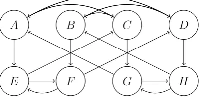
The new IFS has the form ˜F = {f1, ...f20} with the 20 maps corresponding

group of translations. Additionally, it is easy to check that this IFS is still locally rigid. Hence, (F,G) and ( ˜F,G˜) provide two different address space structures for

A B C D

E F G H

Figure 3.3: Substitution golden-b IFS graph

the same system of tilings. The second IFS is an example of what we now define as a substitution IFS.

Definition 3.2. Let the tiling IFS (F,G) be called a substitution IFS if the number of vertices inGcorrespond to the number of prototiles andT is contained in the group of translations. Define ∆ = {Π(θ) +n : θ ∈ Σ†_∞, n ∈ _RM_{} and let}

ω = α−N _{with N ∈ {1, ...a}

max} be the smallest integer so that ω(p) is tiled by

translations of the prototile set for anyp∈ P. Then ωis called the inflation map for ∆.

Observe that all tilings in ∆ are not necessarily in the image of Π. More specifically, ∆ is the closure of _T∞ under the action of translation. We have overloaded the notation ∆ and ω in Definition 3.2 to match the space of tilings and inflation map considered by A & P. We believe that these systems are very similar, if not identical. Now we have a way to express these ideas using the tiling IFS framework.

3.1.2

Space of Tilings

In their paper, A & P require that the space of tilings ∆ satisfies three conditions [AP98]. We consider what these mean in the IFS setting.

- Firstly, they assume that the tiling inflation map is one-to-one. Recall from section 2.3, that local rigidity makes α and α−1 _{into well-defined inverse}

3.1. SUBSTITUTION TILING SYSTEMS 27

- Secondly, they assume that the substitution is primitive: there is a fixed positive integerN0such that for each pair of prototilespi andpj, the partial

tiling ˆωN0₍{p

i}) contains a translation of pj. In the IFS setting, this is

covered by the condition that the graph is strongly connected.

- Thirdly, they require that the space of tilings satisfies a finite pattern con-dition: for any r > 0 there are only finitely many partial tilings up to translations that are subsets of the tiling space and whose supports have diameters less than r. If we replace the requirement by ‘only finitely many partial tilings up to isometry inT’ then all tilings from a tiling IFS satisfy this constraint. This is evident by the existence of the canonical tiling se-quences. The examples that can be expressed as substitution IFS satisfy the stronger finite pattern condition with the translational requirement. Remark 3.3. A & P put a metric on the space of tilings ∆ by saying that two tilings are close if they almost agree on a large ball about the origin. They formally define the metric d for T, T0 ∈∆ by

d(T, T0) = inf({√1

2∪{|T+u and T+v agree on B1(0) for some ||u||,||v||< })

with || · || the usual norm on _RM _{and B}

r(x) an open ball with radius r centred

at x. An argument by [RW92] shows that (∆, d) is a compact metric space. Using a metric equivalent to the one stated above, many researchers in the tiling community consider spaces that are the completion of the orbit of some tiling T. These spaces are denoted by XT and called the continuous hull of T.

The idea is that if T has some nice properties then XT also has nice properties.

The next theorem states some well-known results about XT that are thoroughly

discussed with appropriate references in [Sad05].

Theorem 3.4. Let XT be the continuous hull of a tiling T.

(a) The tiling space XT is compact if and only if T satisfies the finite pattern

condition.

(b) If T is quasiperiodic then the orbit of every S ∈XT is dense in XT.

(c) If T is quasiperiodic and non-periodic then XT locally looks like a disk

For the reader familiar with the language of dynamical systems, part (b) means that XT viewed as a dynamical system by the action of translation is minimal.

A & P show that the tiling spaces they consider are always minimal in this sense (see [AP98, Corollary 3.5]). This result has the important consequence that the space of tilings ∆ is the same as the closure of the orbit of a single tiling by the translational action, i.e. the spacesXT described in [Sad05]. Part (c) tells us that

when the tilings are quasiperiodic and non-periodic the topology of these tiling spaces is highly pathological. The spaces are connected but not path connected. It is also important for the reader to appreciate that there are two different but closely related dynamical systems at play here. Both involve the space ∆ but one is associated with the invertible inflation operation ω and the other is associated with the action of _RM _{by translation.}

Definition 3.5. Two dynamical systems (∆a, ωa) and (∆b, ωb) are topologically

conjugate if there exists a homeomorphism π : ∆a →∆b such that ωa=π−1ωbπ.

One of the main contributions of A & P is showing that the dynamical system (∆, ω) is topologically conjugate to an inverse limit system. To show this topo-logical conjugacy, they construct a CW-complex built from the prototiles of the tiling. The substitution map induces a map from the CW-complex to itself and the inverse limits of such systems turns out to be homeomorphic to the space of tilings. From such a homeomorphism, they show how to calculate cohomology, K-theory and zeta functions for the space of tilings. We narrow our focus to only the first of these computations. Calculating the cohomology of tiling spaces is wide-spread (see [BD08, Sad08] for example) and serves as an important motiva-tion for investigating mixed tiling systems (discussed in secmotiva-tion 5.2).

3.2

Forces its Border

For a tiling space ∆ to be homeomorphic to an inverse limit space A & P require that the tilings satisfy a condition known as ‘forces its border’ [AP98].

Definition 3.6. A substitution forces its border if the following condition holds: there is a fixed positive integer M such that for any tile t and any two tilings

T, T0 ∈ ∆ both containing t then ωM_{(T) and ω}M_(T0_{) coincide on ω}M_{({t}) and}

all tiles that border ωM_({t}).

3.2. FORCES ITS BORDER 29

under translations. For ω = α−2 _{and any tile t, the inflation ω}4_{({t}) in two}

separate tilings containingt will agree on all bordering tiles [AP98]. However, we show in the next section that the Fibonacci tiling does not force its border.

A & P’s idea was to construct a compact CW-complex Γ0 by glueing together

prototiles in all ways in which the substitution rule allows them to be neighbour-ing. This is formalised by the definition below.

Definition 3.8. Let Γ0 = (∆×Rd)/∼be the product space with the equivalence

(T1, u1) ∼ (T2, u2) if tiles t1 and t2 with u1 ∈ t1 ∈ T1 and u2 ∈ t2 ∈ T2, satisfy t1 −u1 =t2 −u2. The equivalence class of a point (T, u) is denoted (T, u)0.

This equivalence relation identifies two tilingsT1 andT2 with specified vectors u1 and u2 if the vectors lie in the same prototile up to translation.

Proposition 3.9. The inflation map ω induces a continuous map γ0 from Γ0

onto Γ0 defined by γ0((T, u)0) = (ω(T), λu)0.

Definition 3.10. Let ∆0 = lim_←−Γ0 be the inverse limit relative to the bonding

map γ0. This means ∆0 consists of all infinite sequences {xi}∞i=0 of points in Γ0

such that γ0(xi) = xi−1. Then a right shift map ω0 : ∆0 → ∆0 is defined by ω0(x)i = γ0(xi). The map ω0 is a homeomorphism and (∆0, ω0) is a dynamical

system.

Proposition 3.11. If the substitution tiling forces its border then the dynamical systems (∆, ω) and (∆0, ω0) are topologically conjugate.

For complete proofs of Proposition 3.9 and 3.11 we direct the reader to [AP98, Proposition 4.2 and Theorem 4.3]. Our main interest is to outline how A & P com-pute the ˘Cech cohomology with integer coefficients of the tiling space Hi_(∆,

Z)

for i ∈ _N0. For an overview of ˘Cech cohomology for tiling spaces and other

versions of tiling cohomology, see [BK10].

Proposition 3.12. If the substitution tiling forces its border then Hi_(∆,

Z) is

isomorphic to the direct limit of the system of abelian groups

Hi(Γ0,Z)−→

γ0∗

Hi(Γ0,Z)−→

γ0∗

· · ·

For a proof of Proposition 3.12 see [AP98, Theorem 6.1]. Since lim_←−Γ0 = ∆0

and ∆0 is homeomorphic to ∆, the following are all isomorphic: Hi(∆,_Z)∼=Hi(∆0,Z) = Hi(lim_←−Γ0,Z)∼= lim_−→Hi(Γ0,Z).

The computation of the direct limit of abelian groups lim_−→Hi(Γ0,Z) is

acces-sible. For 0 ≤ i ≤ M let ci denote the number of cells ci of dimension i in

the CW-complex Γ0. In the cellular cohomology complex for Γ0, the group of

cochains in dimension i are identified with _Zci_{. The cellular map γ}

0 induces a

map on cochains which in dimension i is associated with a ci ×ci integer

ma-trix denoted A0_i. For i = M, the top dimension, the matrix A0_M is exactly the transpose of the cM×cM matrixA(jk) whose entries indicate how many times the

cell j occurs in the inflation of cell k. The maps δ_i0 : _Zci−1 _→

Zci are the usual

boundary maps.

Example 3.13. Summarising results in [AP98], for the golden-b substitution IFS the corresponding cell complex Γ0 has eight faces, eight edges, and three

vertices: ¯F = {A, B, C, D, E, F, G, H}, E¯ = {a, b, c, d, e, f, g, h},V¯ = {α, β, γ}. So δ₁0 : _Z|V¯| → _Z|E¯| _{is an 8×3 matrix indicating the initial and final vertices} for the edges and δ₂0 : _Z|E¯| → _Z|F¯| _{is an 8×8 matrix indicating the edges (with} orientation) that surround the perimeter of each face. The matrices A0₀, A0₁ and

A0₂ indicate how the vertices, edges and faces are respectively subdivided under the inflation map (see [AP98] for the full matrices). We remind the reader that Figure 3.2 displays example subdivisions for faces A and E. The rank of these matrices are

rank(δ0₂) = 2, rank(δ₁0) = 2, rank(A₂0) = 8, rank(A0₁) = 8, rank(A0₀) = 3.

From these ranks and Proposition 3.12 it follows that

H0(∆) ∼=Z, H1(∆) =∼Z4, H2(∆)∼=Z6.

3.3

Collared Tiles

Forces its border turns out to be quite a strong requirement. Many interesting examples, such as the Fibonacci IFS, do not have this property.

3.3. COLLARED TILES 31

a b

1 2

3

Figure 3.4: Substitution Fibonacci graph

(see the graph in Figure 3.4). This presentation matches the representation of the Fibonacci substitution as a system with two rules: a → ab and b → a. So we think of the inflation map ω as taking the tile a to tiles ab and the tile b to a tile a. Let T and T0 be two Fibonacci tilings such that T contains the string

baa andT0 contains the stringaab. Considering inflations of the stringωM(aab), we observe that ωM({a}) is neighboured bybon the left and aon the right when

M is odd and a on both sides when M is even. In contrast, for inflations of the stringωM(baa),ωM({a}) is neighboured bybon the left and aon the right when

M is even and a on both sides when M is odd. So there will never exist an M

such that ωM({a}) coincides on all the neighbouring tiles.

If the tiling does not force its border the map from ∆ to ∆0 in Proposition

3.11 is still well-defined but fails to be injective. Hence, another key idea of A & P was to build a new complex made from tiles together with labels indicating the pattern of neighbouring tiles (called collared tiles).

Definition 3.15. Let t be a tile in T ∈∆, then T1(t) ={t0 _{∈T :t}0_{∩t 6= ∅} is} the collared tile in T containingt.

Definition 3.16. Define

- Γ1 = ∆×Rd/ ∼1 as the product space with the equivalence (T1, u1) ∼1

(T2, u2) if tiles t1 and t2 with u1 ∈ t1 and u2 ∈ t2, satisfy T11(t1)−u1 = T1

2(t2)−u2,

- (T, u)1 as the equivalence class of a point (T, u),

- γ1 : Γ1 →Γ1as the continuous map induced byωand defined byγ1((T, u)1) =

(ω(T), λu)1,

A & P show that (∆1, ω1) is always topologically conjugate to (∆, ω) and

if the substitution forces its border, then (∆1, ω1) is topologically conjugate to

(∆0, ω0) (see [AP98, Theorem 4.3]). Hence, for any substitution tiling, Hi(∆,Z)

is isomorphic to the direct limit lim_−→Hi_(Γ

1,Z) (again see [AP98, Theorem 6.1]).

Example 3.17. Returning to the Fibonacci example (again summarising results from [AP98]), it is clear from inspection that there are only four strings of length three that can occur in any tiling. These correspond to the four collared tiles

{aab, baa, bab, aba}, which we label as{c, d, e, f}respectively. We subdivide these tiles by applying γ1. Slightly abusing notation, we write γ1(c) = (ababa) = ef

where ababa is the expansion of the string c = aab by the usual inflation. We underline the substringabto emphasise that this is the expansion of the prototile

a. We find the collared tiles in the inflation by determining which strings of length three are contained in the set of tiles made from ωN({a}) and its immediate neighbours:

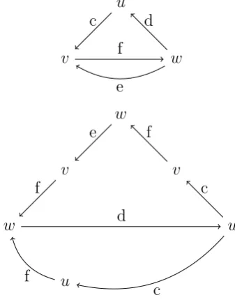
γ1(c) = (ababa) =ef γ1(d) = (aabab) =cf γ1(e) = (aaba) = cf γ1(f) = (abaab) =d.

The complex Γ1is made with three vertices{u, v, w}and the four edges{c, d, e, f}, u

v w

w

v v

w u

u

c f

d

e

e

f

d

c f

c f

3.3. COLLARED TILES 33

as pictured at the top of Figure 3.5. Below, we display the cell complex after in-flation. From this figure, we can read off the values for δ₁0, A0₁ and A0₀. These matrices are

δ₁0 =



   

−1 1 0

1 0 −1

0 1 −1

0 −1 1



   

A0₁ =



   

0 0 1 1 1 0 0 1 1 0 0 1 0 1 0 0



   

A0₀ =



 

0 0 1 0 0 1 1 0 0



 

with rank(δ₁0) = 2, rank(A0₁) = 3, rank(A0₀) = 2. Calculating yields

H0(∆) ∼=_Z, H1(∆) ∼=_Z2.

Remark 3.18. For the IFS setting, switching to collared tiles generates a new IFS. The collared Fibonacci IFS has seven maps Fc={f1, ...f7} and graph with

vertex set {C, D, E, F} corresponding to the four prototiles displayed in Figure 3.6. All the maps have the same scaling factor. Also note that this new IFS is not locally rigid, but importantly it does force its borders. By A & P’s result this means it can be used to calculate the cohomology of the original tiling space.

C D

E F

f2

f1 f4

f3

f5

f6 f7

Chapter 4

Neighbour Graphs

While chapter 3 links the tiling IFS framework to A & P theory, this chapter connects the framework to the study of neighbour graphs in fractal geometry. Both of these connections to the literature are expanded upon in chapter 5 in the discussion of mixed tiling systems.

For the entirety of this chapter, we restrict our attention to iterated func-tion systems where the graph has one sole vertex. So for an IFS of the form

F ={_RM_{;f1, f2, ...f}

N}, the full address space is [N]∗ ∪[N]∞. Letting A denote

the attractor of some IFS, we set Ai := fi(A) for i ∈ [N]∗. Considering two

strings j, k ∈ [N]∗, we can ask whether the corresponding subsets Aj and Ak

intersect. They could intersect at a point, a countable set, an uncountable set, or be entirely disjoint. Studying neighbouring pieces and their corresponding maps has been a long interest of Bandt and various collaborators. They show in [BG92, BHR05, BM09] how the neighbour map theory allows one to check the ‘open set condition’ (defined in 4.1), describe properties of the fractal including connectness and boundary dimensions, and view the fractal as the quotient of a symbolic space.

Section 4.1 introduces the neighbour map theory, with a particular emphasis on showcasing an interesting example from [BM18]. As far as we know, the theory is only thoroughly developed for systems whose maps have uniform scaling factors. In section 4.2, we propose an extension of the theory to cover the case when the IFS maps have scalings that are integer powers of some 0 < s < 1. From this extension, we can apply the neighbour map theory to study a wider range of tiling IFSs. The Sierpinski, rigid Williams, Fibonacci, and golden-b all make appearances.

4.1

Uniform Scaling

To introduce neighbour maps and graphs, we consider an IFSF ={_RM_;f

1, f2, ...fN},

where each fi is an invertible contractive similitude with scaling factor 0 < s <1.

In this setting, neighbouring pieces to the attractor A are always isometric to A

itself.

Take strings i, j ∈ [N]∗ such that |i| = |j| and consider maps of the form

h=f_i−1fj. The maph takes A onto its potential neighbour h(A), which has the

same position with respect to AasAj does withAi. The maph=fi−1fj is called

a proper neighbour map if Ai ∩Aj 6= ∅. These neighbour map are generated

recursively. Starting with maps of the form h1 = fi−11fj1 with i1 6= j1 ∈ [N],

we find further maps by setting h2 = fi−21h1fj2 for i2, j2 ∈ [N]. This process

continues, and in fact all neighbour maps are obtained by applying the interior automorphism Φij(h) =fi−11hfj1 for i, j ∈[N] starting with h=id [BM09].

Definition 4.1. For the uniform scaling setting, define the set of proper neigh-bours as

N ={f−1

i fj :i, j ∈[N]∗,|i|=|j|, fi(A)∩fj(A)6=∅}.

The neighbour graph is constructed by setting the vertex set to be the set of proper neighbour maps. There is a directed edge, labelled (i, j), from vertex h

to vertex ¯h if ¯h = f_i−1hfj for some i, j ∈ [N]. The identity map id denotes the

root vertex of the graph but by convention it is not included in the figures and all edges from the root have no initial vertex. An IFS F is said to be of finite type if there are only finitely many proper neighbour maps and hence only finitely many vertices in the neighbour graph [BM09].

For (j, k)∈[N]∗the setf_j−1fk(A) is called a neighbour ofAandfj−1fkreferred

to as the corresponding neighbour map. The intersection f_j−1fk(A)∩A of the

fractal A with its neighbour is called an edge of A. Definition 4.2. An IFS F = {_RM_;f

1, f2, ...fN} is said to satisfy the open set

condition (OSC) if there exists a nonempty open set V ⊂_RM _{such that} N

[

i=1

fi(V)⊆V and fi(V)∩fj(V) =∅ for i6=j.

4.1. UNIFORM SCALING 37

Example 4.3. To get a feel for how to construct neighbour graphs, we begin by considering the Sierpinski IFS, F ={f1, f2, f3}, defined in section 2.3.1. Though

we have not seen this neighbour graph presented explicitly before, for anyone familiar with neighbour map theory it would be an easy computation. To find the set of proper neighbours, we consider the ways an isometric copy of the attractor A can intersect Π(∅). With Π(∅) shaded in red, Figure 4.1 shows that there are six ways, corresponding to the existence of six proper neighbour maps. The complete set of non-trivial neighbour maps for the Sierpinski IFS is

N ={f−1

1 f2, f2−1f1, f1−1f3, f3−1f1, f2−1f3, f3−1f2}.

So the neighbour graph has six vertices which we label asr=f₁−1f2,r− =f2−1f1,

Figure 4.1: Sierpinski neighbours

s = f₁−1f3, s− = f3−1f1, t = f2−1f3, and t− = f3−1f2. The pairs (Aj, Ak) for

j 6=k intersect on a point, so there is only one subpiece (Ajj0, A_kk0) for some pair

(j0, k0)∈[3]×[3] such that Ajj0 ∩A_kk0 6=∅.

Consider the neighbour map r = f₁−1f2 which maps A1 to A2. We observe

explicit functions. So we have a loop labelled (2,1) on r in the neighbour graph. We find such loops for all the other vertices, yielding the full neighbour graph as displayed in Figure 4.2.

r _r−

s _s−

t t−

(2,1) (1,2)

(3,1) (1,3)

(3,2) (2,3) (1,2)

(1,3)

(2,3)

(2,1)

(3,1)

(3,2)

Figure 4.2: Sierpinski neighbour graph

It is well known that the symbolic space quotiented out by the set of equivalent addresses is homeomorphic to the attractor itself. Let r ∼t if π(r) =π(t), then

π : [N_∼]∞ → A is a homeomorphism [Bar93]. Recall that the coding map from Theorem 1.12 is surjective but not generally injective. In [BM09] Bandt and Mesing state that “pairs of equivalent addresses coincide with labelled sequences of infinite edge paths in the neighbour graph”. Their proof is short and we believe a more thorough and explicit justification of this equivalence is clarifying. Proposition 4.4. The following is true: π(r) = π(t) if and only if for some

n ∈ _N, r1...rn−1 = t1...tn−1 and h = fr−n1ftn is a proper neighbour map with an arrow to it from the identity vertex and (Sn_{(r), S}n_{(t)) coincides with a sequence}

of infinite edge paths starting from h in the neighbour graph.

Proof. The backwards direction is easy. Assuming r1...rn−1 = t1...tn−1 and h = f−1

rn ftn is a proper neighbour map means thatAr1...rn∩At1...tn 6=∅. Then following

an infinite edge of paths from this vertex implies thatAr∩At6=∅, soπ(r) =π(t).

For the forward direction, supposing r 6= t ∈ [N]∞ with π(r) = π(t) gives us that Ar∩At 6= ∅. The points Ar and At either lie in a single copy Ai or on

the boundary of multiple sets Ai for i ∈ {1,2...N}. If they lie in a single copy

Ai1, then set r1 =t1 =i1. Next, consider the sets of the form Ai1j and check for

4.1. UNIFORM SCALING 39

until the points eventually lie on the intersection of at least two sets. Say this is at stage n∈_N, then label two of the different indices of the sets that the points are bordering as k 6= l ∈ {1,2...N}. We set rn =k and tn = l and observe that

h = f−1

r1...rnft1...tn = f

−1

rn ftn is a proper neighbour map which has an arrow to it

from the identity vertex in the neighbour graph. Since π(r) = π(t), from vertex

hthere is an infinite path in the graph (Sn_{(r), S}n_{(t)) that corresponds to the tail}

of strings r and t.

This proposition says that a purely symbolic description of the attractor can be obtained from the neighbour graph. From the graph, we can determine all the equivalent addresses of points on the attractor. By Example 4.3 and Proposition 4.4, all equivalent addresses in the Sierpinski attractor end in pairs (1¯2,2¯1),(1¯3,3¯1) or (2¯3,3¯2).

Now, we shift our focus to recent work by Bandt and Mekhontsev who recently discovered some new relatives of the Sierpinski gasket [BM18]. The IFSs for these relatives are all generated by three maps:

fk(z) =

1

2sk(z+ck) fork = 0,1,2

where ck =ak+ibk with ak, bk ∈Z, the points {c0, c1, c2} are non-collinear, and

sk ∈ {id, s(z) = iz, s2(z) = −z, s3(z) = −iz}. So the maps are integer

transla-tions with a rotation around 0,±90◦ or 180◦ with scaling factors 1₂. Additionally, they require that the IFS satisfies the open set condition. The Hausdorff dimen-sion of all these relatives’ attractors is log(3)_log(2) ≈1.585. Alongside showcasing some well known examples including the Sierpinski triangle and the two dimensional Cantor set, they present some new examples that satisfy these constraints. The simplest new example they describe is called ‘Crossings’. This example nicely demonstrates how the neighbour graph can be used to compute properties of the fractal including connectedness and boundary dimension. All the results and computations for this example follow [BM18].

Example 4.5. Let F ={f0(z) = −₂iz, f1(z) = −₂1(z−1−i), f2(z) = −₂1(z+ 1)}

be the Crossings IFS with attractor A displayed in Figure 4.3. We observe from Figure 4.3 thatA1andA2differ by a translation. Lett=f1−1f2be the translation

taking A1 to A2 computed as t(z) = z−2−i. Let t− = f2−1f1 be the inverse

which translates A2 to A1 by t−(z) = z + 2 +i. Note that A12∩A21 6= ∅ and A12 is mapped to A21 byt− since there is a 180◦ rotation in the mapsf1 and f2.

Figure 4.3: Crossings attractor [BM18]

graph, there is an edge labelled (1,2) from t to t− and by a similar computation there is another edge (2,1) from t− to t.

Other neighbour maps arer =f₀−1f1 and u=f0−1f2 and their inverse. Going

a level deeper, we find that A00 maps to A11 by the map s(z) = −z + 1 which

is self-inverse; s = s−. It turns out that these seven maps are all the possible neighbours. The set

N ={t, t−, r, r−, u, u−, s},

see Figure 4.4, is complete since for any h ∈ N and any pair j, k ∈ {0,1,2} the map ¯h=f_j−1hfk is also in N. By the same methods as before, we find the edges

between the vertices and complete the neighbour graph (displayed in Figure 4.5).

Figure 4.4: Crossing neighbours [BM18]

4.1. UNIFORM SCALING 41

t t−

s

u _u−

r _r−

(1,2) (2,1)

(1,2) (2,1)

(0,1)

(1,1) (1,2)

(1,0)

(1,1) (2,1)

(2,0) (0,2) (0,1)

(0,2) (2,0)

(1,0)

Figure 4.5: Crossings neighbour graph

can read off that 1 ¯12 and 2 ¯21 are equivalent addresses corresponding to the single point of intersection between A1 and A2. We also observe the lower connected

portion of the Crossing neighbour graphs has several cycles with a common vertex. By [BM09], A0∩A1 and A0∩A2 are Cantor sets.

The edge corresponding to a neighbour map is denoted by the capitalisation of the map’s label. For example, the corresponding edge for the mapr=f₀−1f1 is denoted byR =r(A)∩A. We know from above thatRis a Cantor set but it turns out that from the neighbour graph its dimension can be computed explicitly. The edges themselves are self-similar, made from copies of other edges with one of the maps f0, f1, f2 applied. Since two edges from vertex r are directed to vertices u

and s, the edge R is made from self-similar copies of the edges U and S. The vertex u has only one outgoing edge, labelled 1 directed to r. The vertex s has an edge labelled 2 to u and 0 to u−. This yields the equations

R=f1(U)∪f0(S), U =f1(R), S=f2(U)∪f0(U−).

The edge U− is isometric to U by an isometry we label u−. Then

R=f1f1(R)∪f0(f2(U)∪f0(U−))

=f₁2(R)∪f0f2f1(R)∪f0f0u−f1(R)

So R is a self-similar set that is the union of maps with scaling factors {1 4,

1 8,

1 8}.