A computer based feasibility analysis of assessing arterial flow using pulsatility indices

1-1-1982

A computer based feasibility analysis of assessing

arterial flow using pulsatility indices

Gerold Porenta

Iowa State University

Follow this and additional works at:

https://lib.dr.iastate.edu/rtd

This Thesis is brought to you for free and open access by the Iowa State University Capstones, Theses and Dissertations at Iowa State University Digital Repository. It has been accepted for inclusion in Retrospective Theses and Dissertations by an authorized administrator of Iowa State University Digital Repository. For more information, please [email protected].

Recommended Citation

Porenta, Gerold, "A computer based feasibility analysis of assessing arterial flow using pulsatility indices" (1982).Retrospective Theses and Dissertations. 18682.

A computer based feasibility analysis of assessing

.f$1-I

/

'7

,,~

,,,..,

~ fl' r) '5. ·" , if - '

e,

3'

arterial flow using pulsatility indices

by

Gerold Porenta

A Thesis Submitted to the

Graduate Faculty in Partial Fulfillment of the Requirements for the Degree of

MASTER OF SCIENCE

Major: Biomedical Engineering

Signatures have been redacted for privacy

Iowa State University Ames, Iowa

1982

1420656

I

TABLE OF CONTENTS

INTRODUCTION LITERATURE REVIEW

Models of Blood Flow in Arteries

Diagnostic Methods for Measuring Arterial Flow Noninvasive Assessment of Arterial Flow

THEORETICAL MODEL . . . Governing Equations Numerical Procedure

Pulsatility and Area Indices PHYSIOLOGICAL MODEL . .

INTRODUCTION

In 1978, cardiovascular diseases accounted for 51.3% of all deaths

in the United States (U.S. Department of Health and Human Services,

1980, p. 26), and to date they still pose the country's most serious health problem. The direct economic cost of illness for these diseases,

that touch the life of virtually every American, amounted to 50 billion dollars in 1975 (U.S. Department of Health and Human Services, 1980, p. 33). Consequently, a major research effort has been directed towards

the study of var{ous forms of cardiovascular disease, such as

atherosclerosis, cerebrovascular disease, coronary heart disease, and peripheral vascular disease. As a result, important research advances

have contributed to a significant decrease in the cardiovascular death

rate.

Arterial diseases are the subject of many investigations, as they are closely related to many other cardiovascular diseases. For example, the partial occlusion of a coronary art"ery can reduce the blood supply to the heart and lead to a myocardial infarct. A constriction of arteries supplytng the brain with blood can result in a cerebral accident (stroke). Frequently, the narrowing of an arterial lumen

Identification of risk factors has made possible an improvement of

preventive actions over the past years. It appears that the public has become more aware of known cardiovascular risk factors and has adjusted behavior and lifestyle to reduce a number of risks such as the use of

tobacco products and the consumption of high saturated fat-high

cholesterol foods (U.S. Department of Health, Education, and Welfare,

1979, p. 2). Many aspects of the etiology of cardiovascular diseases,

however, remain unknown, so that the implementation of a comprehensive and effective prevention program has been impossible to achieve so far.

Once a disease develops, successful therapy and cure often depend on an early and accurate diagnosis, not yet available for many

cardiovascular diseases. Peripheral arterial diseases, which frequently

do not exhibit clinical symptoms during the early stages, can remain undetected until more than 90% of the artery's lumen is occluded. At this late stage in the disease process the treatment is usually a

surgical procedure, as compared to pharmacological treatment that could be used if the dJsease were diagnosed during the early stages. Today

several diagnostic techiliques are available, differing in two usually mutually exclusive aspects: efficacy and patient safety.

Arteriography, an invasive diagnostic technique, is generally

considered to be more reliable than various noninvasive methods, but has a disadvantage since it involves a surgical procedure with an associated risk. Ultrasonic techniques, on the other hand, are noninvasive and can

particular patient.

One diagnostic method utilizing ultrasound is based on the changes

in the flow waveform that occur in diseased arteries. A puisatility index, commonly defined as the r!ltio of the peak to peak ve1ocity excursion to the mean velocity, is measured distal and proximal tq the obstruction. The ratio of these. two indices, called the inverse damping

factor, or simply the magnitude of a given pulsatility index can presumably provide some indication of the presence of a pathological situation. This. method has been used successfully in clinical

situations, but a detailed analysis of the effect of various parameters

such as taper and branchi11-g': _of arterie'>, measurement site, and blood viscosity on the pulsatility index has not yet been accomplished.

The purpose of this thesis is to develop a computer model of the

human femoral artery and to use this ·model to (1) study the influence of various flow situations on generalized pulsatility indices and their corresponding inverse· damping factors, and (2) investigate the

feasibility of usin_g these indices to predict the presence of a s.tenosed arterial segment.

In the literature review, I will (1) summarize different approaches taken in modeling arterial blood flow, (2) comment on the

instrumentation available to m_easure blood flow in arteries, and (3) provide info.rmation on clinical applications which utilize pulsatility

indices to detect abnormal flow situations. I will then present the basic equations of th<> theoretical model_, explain the numerical

the pulsatility indices investigated in this study. The chapter on the physiological model will contain a description of geometry and

properties of the human femoral artery and the values of system

parameters. A discussion of results followed by a suminary will conclude

this thesis.

LITERATURE REVIEW

The following literature review is not meant to be comprehensive, as the literature on the three topics presented is so extensive that it would be far beyond the scope of this thesis to provide a complete

review. Rather I will present the basic equations used in

cardiovascular modeling, establish a frame of reference relating my model to its predecessors, and focus mainly on publications· stressing· an

interrelation between modeling and clinical situations.

Models of Blood Flow in Arteries

Most of the model studies are based on three types of equations:

the Navier-Stokes equation, the continuity equation, and an equation of state. 'Therefo:re, this review first provides a general discussion of these equations followed by a presentation of different applications appearing in the literature.

·For more than 2000 years, blood flow in arteries has been a major point of research for many investigators with very different

professional origins. But progress was very slow, and many functional features of the arterial system were still unknown in the 16th century when the classical Galeµical teaching that blood was created in the

liver and absorbed by the tissues to which it was conveyed with

oscillatory motion mainly in the veins prevailed (McDonald, 1974, p. 4). Essential discoveries did not come about until the 19th century when experiments were conducted more meticulously and mechanical principles were app1ied to cardiovascular flow situations. Using

theoretical considerations, Navier and Stokes derived an equation

describing both steady and unsteady laminar flow of a Newtonian fluid. In formal mathematical terms, the Navier-Stokes equation can.be written

as:

m (

_at

₊

_{q. q} V)

_{+ "P}

1

v

_{P -} B _{- ; q} µV2 ₌ 0 (1)

where q is the flow vector, p the pressure, p the fluid density, µ the fluid viscosity, and B an external body force vector. This nonlinear

partial differential equation, capable of describing very general flow situations, still defies an analytical solution in its most general form, more than 130 years after the first publication.

Another basic law in fluid mechanics is the continuity equation stating that fluid mass' flowing through~ control volume cannot be lost

or transformed within the control volume, or in other words: mass flowing into a control volume must be balanced by the mass flowing out

of it. The mathematical notati?n is given by

V.q ·= 0 (2)

If applied to laminar flow of an incompressible fluid in a tube with

rigid walls, the continuity equation indicates that the volume rate of flow is independent of position and therefore changes with time

uniformly along the tube.

for the flow problem. The resulting velocity profiles provide an

approximation to pulsatile blood flow and correctly indicate that flow reversal (arterial flow from the periphery to the heart) can. occur during the cardiac cycle, a finding well documented by in vivo studies.

Womersley's solution cannot be written in terms of explicit functions; it requires that the driving pressure be specified as a

Fourier series, and each term in the Fourier series yields a

corresponding flow term containing Bessel functions. That makes the

solution somewhat awkward to work with. Nevertheless, Womersley's· work

is one of the milestones in modeling blood flow in arteries and has provided the foundation for an improved understanding of processes in the cardiovascular system. Shortly after Womersley published. his

research, analog and digital computers became more widely available, and many investigators took advantage of these new tools giving rise to a new branch of cardiovascular modeling presented later in this section.

A different approach to modeling originated from the science of maj:erial properties, which started in the first half of the 19th century

when Thomas Young the famous biophysicist did work on the nature of elas.ticity. He was particularly interes.ted. in the relation between the elastic properties of arteries and the velocity of propagation of the

arterial pulse. A similar problem is to find a relationship between the cross sectional area of an artery and its distending pressure.

An

Experimental studies (Roach and Burton, '19.59; Boughner and Roach, 1971) relate the circumferential tension T and the percent increase in circumference of an a:i::.tery, With the use of Laplace's law

T

=

pR

wh.ere p is ·the distending pressure and R the arterial radius, the

tension strain curves can then be rewritten in terms of area and

pressure if the value for the radius of the unstrained. artery is known. A theoretical analysis can deduce an equation 'of state· from

mechanical principles valid for thin walled vessels. Depending on the assumptions made during the derivation, different results will be

obtained. Streeter et al. (1963) assumed the vessel to have a constant volume per unit length and the vessel material to be incompressible

(Poisson's ratio

=

O. 5) and presented an equation of state in the following form:

(3)

where A(p,x) is the area as a function of pressure p and arterial length x, E is the modulus of elasticity, and d0, h0 are the values of vessel diameter and thickness at a reference pressure p0. For clinical

application, this equation is of limited value since equipment to measure the modulus of elasticity in vivo is not yet available.

Equatidn .(3) can be modified by introducing a new parameter, which

=

(Eh/· d) 0 ' 5

ao

o

P o (4)

which originated from work on wave propagation in the last century. The

Moerts-Korteweg equation in.a strict sense is valid only for nonviscous fluids., but it does .provide a good approximation for blood :flow. A substitution of equation (4) into equation (3) yields

2 -1

A(p,x)

=

A(p

₀

_{,x)(l-(p-p0)/pa0 )}

leaving only two parameters, the fluid density and the pulse wave

velocity.

(5)

Another· parameter easily obtainable in clinical situations is a pressure strain modulus E defined as E _{p p} = (R/LIR)llp. Mozersky et al.

(1972) transcutaneously measured E on patients classified in three _p different age groups· and found an increase of E with age. They also _p observed large variations within the age groups. By integrating the definition of E , an equation of state in _{. p} t~e form

A(p,x) = A(p

0,x)e2(p-po)/EP (6)

Efforts to model one dimensional arterial flow on computers started

two decades ago on analog computers where simplified and linearized

equations were implemented. As more sophisticated algorithms became available to solve partial differential equations on digital computers,

the research emphasis shifted towards digital computers, partly because nonlinearities can be included with relative ease.

Snyder et al. (1968) set up a linear model of the systemic

arterial.-tree on an analog computer and obtained results that agree with

physiological data ·such as distal delay and peaking of pressure pulse

waves. Moreover, several clinical parameters such as cardiac output and cardiac work were investigated with respect to variations in the -heart rate.

Westerhof et al. (1969) used a linear model to build an electric analogy of the total human systemic arterial tree. They discuss several concepts of vascular impedance and wave travel and prove that a s-imple

aortic model .consisting of a single tube with only one distal reflection site at its end does not accurately represent the physiological

situation. The peripheral peaking of the pressure pulse is attributed to reflections for lower harmonics at the peripheral beds simulated by a

lumped pure _resistaI1ce. Westerhof et al. neglect viscoelastic behavior and, for clinical comparisons, simulate effects of essential and old age hypertension.

convective acceleration term in the Navier-Stokes equation. In more detail, Schaaf and Abbrecht attribute the main differences to the

nonlinear effects of finite wall displacements and only small influences to the terms in the Navier-Stokes equations corresponding to convective acceleration and fluid friction. The influence of the peripheral beds

are accounted for by including-a distal lumped resistance.

Wemple and Mockros (1972) used the methods of characteristics to implement a nonlinear model' on a digital computer by including

convective acceleration and fluid friction for steady and first harmonic

sinusoidal flow in the Navier-Stokes equation and by allowing the

modulus of elasticity in the equation of state to be a function of cross sectional area (elastic taper). Simulation of.the peripheral beds in this model is more e_laborate than in the models presented above, as it provides for both resistive and .compliant components. Like Snyder _et al. (1968), Westerhof et al. (1969), and Schaaf and Abbrecht (1972), Wemple and Mockros concentrate on the behavior of the pressure pulse wave and try to determine its governing factors. From their results,

Wemple and Mockros conclude that reflections at the distal end are mainly responsible for pulse wave amplification, whereas geometrical taper does not exhibit a major influence. Wemple and Mockros also suggest that elastic taper and nonlinearities in the wall elasticity do

not significally alter pressure and flow profiles. For low frequencies, their nonlinear model deviates only slightly from the linear model.

close to the in vivo situation. In assessing the various effects of paramete:i; variations on almost exclusivly the pressure waveform, they retain the nonlinearities in the governing equations. Many diffen:nt physiological conditions are simulated during the sensitivity analysis. Networks of a resistance in s.eries with a parallel combination of a

resistance and a compliance account for the effects of two branches and

the a~terial tree distal to the popliteal artery. The terminating

networks can be physiologically interpreted by attributing the effects of the first resistanc;e to. the flow resistance located in the arterioles

and the effects of the parallel combination to the influences of the capillary bed. From the sensitivity.analysis, Raines et al.. deduce that the pressure waveform ·.is only moderately affected by the convective

acceleration, blood viscosity, and branching, but that vessel elasticity and' distal reflections strongly determine the behavior of the pressure pulse. These results are in good agreement with Schaaf and Abbrecht

(1972) and Wemple .and Mockros (1972).

Overall, the basic model of the human femoral artery as presented by Raines et al. (1974) includes all the main features known to

determine flow and pressure waveforms, and at the same time provides a model geometry and a set of parameters that simulates rather closely the

Diagnostic Metliods for Measuring Arterial Flow

The most common diagnostic method is arteriography, an invasive method where a radioactive tracer material is injected into the artery and x-ray pictures are taken providing information about the presence of

a constriction. This method is considered to be the most reliable diagnostic technique; however, it is relatively time consuming,

expensive, cannot be used repeatedly for routine screening and followup

examinations, is associated with a certain degree of morbidity and mortality, and may indicate less arterial obstruction than is present

(Lee et al., 1980). In an attempt to overcome these difficulties, noninvasive techniques have been developed based on the abnormal flow characteristics that develop in stenosed arteries.

Electromagnetic flowmeters, in the past used only on exposed arteries during surgery, now are used noninvasively by creating the magnetic field exterior to the body. Lee et al. (1980) reported on the

successful application of a noninvasive calibrated electromagnetic flowmeter in assessing arterial peripheral flow.

Ultrasonic devices are the most frequently used noninvasive diagnostic instruments in a clinic~l environment. One ultrasonic technique produces scans of arteries by colouring images according to the peak velocity at each point in the artery. Abnormalities are identified by change of flow velocity rather than direct visualization of vessel narrowing. Another device displays all frequencies occurring

turbulent flow, energy is spread over a wider frequency range. The

physician then deduces from the distribution of energy the flow

situation.

Ultrasonic flowmeters which provide a measurement of the flow

waveform at one specific point of the artery during a cardiac cycle have been used extensively to assess peripheral arterial.flow (Gosling et

al., 1971, Harris et al., 1974, Johnston et al., 1978, Baird et al.,

1979). Two techniques, the continuous wave Doppler flowmeter (CW Doppler) and the pulsed Doppler flowmeter, differ in the way the flow

waveform fa obtained. The CW Doppler measures velocity comp.onents over the total arterial cross section, which are used to generate a

representative wave sample. Johnston et al. (1977) point out problems associ11ted with the use of CW Dopplers and present solutions to overcome these problems. Pulsed Doppler flowmeters concentrate on a restricted area of the total arterial lumen, and depending on the size of an artery, can be used to obtain flow waveforms at several sites between the ·arterial wall and the arterial center. Baird et al. (1979) measured

flow waveforms with a 30 channel pulsed Doppler flowmeter at 4 points

across the section of the femoral artery.

At the present time, .both CW and pulsed Doppler flowmeters are

difficult to calibrate. accurately, and their output waveforms are

Noninvasive, Assessment of Arterial Flow

All of the following methods for assessing arterial flow are based on the evaluation.of flow waveforms obtained with uncalibrated

ultrasonic equipment.

Arterial obstruct,ions cannot be detected by ultrasonic· methods unless they cause changes in the flow behavior. Often, stenoses are

thought to dampen the flow waveform and reduce the pulsatility of blood flow along the artery. During the past ten years, several methods have been introduced to associate a pulsatility index with flow waveforms and

to deduce the flow situation from variations of the pulsatility index along the artery. Because of easy accessibility, the arteries in the

human legs have served as a benchmark for the different methods. Gosling et al. (1971) were the first to use a pulsatility index (PI) defined as the total oscillatory energy in the flow velocity

waveform divided by the energy of the mean forward flow velocity during a cardiac cycle. 'By looking at the variation of the PI from the

abdominal aorta to the tibial arterie,s, Gosling et al. could arrive at a quantitative comparison of the arterial pathway capabilities of

different patients.

Woodcocl<; et al. (1972) introduced the damping factor (DF) as the ratio of proximal and dis~al measured Pis and tried to relate the DF with pressure drop and flow. Their results indicate that the DF method

could quantitatively correlate the DF with the degree of arterial

obstruction.

Harris et al. (1974) studied the relationship between an assessment

using the pulsatility index and angiography in occlusive arterial diseases in the human limbs. Their work led to the conclusion that assessments of disease by the 2 methods correlate, but that the

ultrasound method could incorrectly disclose a severe disease which was not apparent in the angiography.

According to the original definition of the PI, its evaluation

requires the flow waveform to be presented in Fourier coefficients, thereby making necessary a conversion of flow data from the time to the frequency domain. Thus, Gosling and King (1974) trying to overcome this computational disadvantage defined a pulsatility index as the ratio of peak to peak flow excursion to the mean flow. This PI with the same

information content as the previous one (Gosling and King, 1974; Johnston et al., 1978) is easier to evaluate. Subsequent studies

(Johnston and Taraschuk, 1976; Johnston et al., 1978; Baird et al., 1979, Evans et al., 1980) made use of this new definition of the PI.

Johnston and Taraschuk (1976) compared the PI method with graded

arteriograms and ankle systolic pressure measurements. Their results suggest that the PI method is capable of detecting clinically

significant stenoses (more than 50% area obstruction) and may be

investigated patient group.

In a later study, Johnston et al. (1978) comment on problems associated with the CW Doppler device hardware, present an improved system, and demonstrate that clinically significant peripheral arterial

occlusive disease can be quantified and regionally localized with the PI

method. Also, the authors prefer to use the inverse damping factor (IDF) because like most clinical measurement indices it decreases with

increasing disease state. Moreover, the IDF (with a fixed proximal PI and a:·varying distal PI) plotted against arterial tube length shows the behavior of a normalized pulsatility index along the artery in a

proportionate fashion (independent variable in the numerator of the' ratio) as opposed to the inverse proportional plot of the DF along the

artery .. For most people, proportional curves are easier to interpret. For these two reasons, I chose t'o investigate the behavior of the IDF

instead of the DF which is more common in the literature.

Baird et al. (1979) working with a 30-chaimel pulsed Doppler flowmeter scanned the pr9funda branch of human femoral arteries and

found that a stenosis of more than 50% was invariably associated· with a IDF of 'less than 0.67. For normal limbs, the IDF was always greater than 0. 71.

at the same time all but the tightest stenoses exhibit a wide scatter in

the results, an effect attributed to the influence of peripheral resistance. Therefore,, the dependency of the PI on the peripheral resistance is much more marked in the case of mild st;enosis, whereas

tight stenoses always result in a low PI. In the animal model, only stenoses greater than 86% produced an PI low enough to be diagnostic of

inadequate flow.

The study of Evans et al. (1980) shows clearly that the diagnostic value of the PI method depends significantly on an accurate knowledge of

its sensitivity to parameter variations.

A

detailed sensitivity analysis, however, cannot be performed in animal models. Therefore, I studied the sensitivity of the PI method on a computer model and

THEORETICAL MODEL

Governing Equations

· Three equations describing general fluid flow situations were presented in the previous·chapter: momentum equation, continuity

equation, and ail equation of state. The three independent variables in

these equations are the three dimensional flow vector q(x,t), the pressure p(x,t), and the cross sectional area A(p,t). For.the purpose of th:i.s study, all ·three equations were modified to obtain a description

of arterial blood flow that can be treated numerically with relativt;)

ease.

The Navier-Stokes equations can be reduced to an equation of·the

form

(7)

by integrating equation (1) over the arterial cross section and making the following assumptions:

L ·Arterial flow is axisymmetric.

2. The blood layer adjacent to the arterial wall follows the wall motion ('no slip' condition).

3. The pressure is uniform across the arterial cross section.

4.

The wall stress for arterial .flow can be approximated by the wall shear stress for steady flow.

5. The second derivative of the axial flow component with

The second and third term in equation (7) are the convective

acceleration terms, and the last term is the fluid friction term. In

the following, equation (7) will be referred to as momentum equation.

The continuity equation c.an also be integrated over the arterial

cross section. By neglecting flow through the arterial wall (seepage)

and using the'' first two assumptions from above, the following equation

can be obtained·:

~

+

aA = ₀

ax at

(8)

The two forms of an equation of state given in equations (5) and

(6) include a type of nonlinearity that is not well-suited for the

numerical algorithm of finite elements used in this study. Therefore, I

chose to work with' an approximation in the form of a second order

polynomial

A(p,x) (9)

The coefficients of the polynomial

C~

and

C~

can be found by rewriting

equation (5) as a geometrical series or expanding equation (6) into a

Taylor series and neglecting terms of higher order. Alternatively,

fitting equation (9) t'o pressure area curves from experimental studies

also yields values fqr the coefficients. In any case, the resulting

approximation has· to be examined carefully with respect to accuracy.

For example, the validity of equation. (5) in a rigorous sense is. assured

only for small pressure variations around a reference pressure p 0. An

approximation of the equation of state based on equation (5) will

pressure where the mean arterial pressure is taken as p0. Compared to the assumptions included in the derivation of· equations (7) and (8), the

approximation of the ~quation of state by equation (9) probably introduces the most significant deviation from the physiological

situation.

To obtain two equations containing partial derivatives with respect to only two independent variables,. equation (9) can be used to eliminate the area derivative in equation (8). After the substitution, the

continuity equation has the form

(10) .

where

C ₁

=

2Ca ₁

Equations (7) and (10) constitute the governing equations of blood flow in unobstructed arteries without branches.

To simulate an arterial sectioJ;I that includes a branch diverting

from the main stem, two equations are needed to replace equations (7)

and (10). The effects caused by a branch are usually lumped into equations containing parameters that account only for the overall

hemodynamic behavior and do not provide a detailed'flow description such as equations (7) or (10). As a good approximation, the small pressure drop across the branch location can be neglected.

~

_ax

=

0

Thus,

takes the place of the momentum equation. The form of the second equation which includes the effect of branch flow depends on the model adopted for the peripheral beds. In many studies, this is chosen to be

a pure lumped resistance'. However, Raines 'et al. (1974) stated that the compliant contribution' of the. peripheral beds plays a role in

determining the distal pulse wave form; consequently they used a network

which includes a resis.tance R1 in series with the parallel combination of a resistance RZ and a co~pliant element C to simulate peripheral

beds.

t

also considered this constellation to be more realistic and incorporated it into my model. With the assumption that the venous pressure is· zero, the equation for the branch flow B is

(12)

From the continuity principle, it follows that B is the difference between the flow before and after .the branching point in the main arterial stem. At the distal end, the flow rate in the main artery obeys the same equation as B in equation (12).

In addition to unobstructed arteries, stenosed arter.ies will also be simulated in this study. Thus, two more equations are needed that

involve the pressure drop across the stenosis and the corresponding volume rate of flow. If the stenosed arterial section is considered to be noncompliant, the, continuity equation (8) reduces to

aq

=

o

(13)

ax

which gives the first of two required equations. The second equation is

tubes with different types of obstructions and combined theoretical and

experimental data to develop the relationship

and

where llp is the pressure drop across the stenosis, A0, D and A1, D1 are the areas and diamete~s of the unobstructed and obstructed arterial lumen, respectively; and 1 is the length of the stenosis. In my model,

Kt and K were assigned the values 1.5 and 1.2. These empirical values _{u .} correspond to stenos es having the shape ·of blunt ended, holli;>wed plugs.

A derivation of this equation and a discussion of various hemodynamic factors pertaining to blood flow in stenosed arteries are given in Young

(1979).

In summary, a pair of equations containing the partial derivatives of flow and pressure with respect to time and position have been

presented for three different model situations: unobstructed artery without a branch, unobstructed artery including a branch, and

obstructed artery. Given a description of the model geometry and a specification of proper boundary values, a numerical solution to these

Numerical Procedure

The ·governing equations of the model include nonlinear terms and thus cannot be solved.analytically. Instead, numerical methods that can be implemented on a· digital computer have to be used to provide an

approximate solution. Most numerical methods are based on a discretization process where the derivative terms in the partial

differential equations are replaced with algebraic expressions. lf the

discretization process is carried out in accordance with certain

restrictions, the solution to the system of algebraic equations

represents an accurate approximation to the analytical solution of the

partial differential equations.

In my model, several sets of partial differential equations

interact with each other, corresponding to the differences in arterial sections (without a branch, with a branch, and with a stenosis).

Inhomogenous model geometry like this can be treated with relative ease

by the numerical method of finite elements. Rooz (1980) gives a

detailed step by step description of applying the finite element method

using the Galerkin method to.equations simulating blood flow. Over~ll, this method is not only well-suited to discretize flow equations, but it is also relatively easy to implement. Therefore, I extended his

approach to the more general equations of this study.

In the Galerkin method, the domain of the independent variables, location and time, is divided into rectangular elements with four nodes

Q(x,t) = [N(x,t)]{q} (15)

and

p(x,t) = [N(x,t)]{p} (16)

where {q} and {p} are four dimensional column vectors consisting of the

unknown flow and pressure values at the four nodes, and [N(x,t)] is a four dimensional row vector of the shape functions N.. The N. are _{l. l.}

chosen so· that they assume the value 1 at node i and 0 at the three other nodes. After substitution of equations (15) and (16) into a pair of corresponding differenti'll equations such as (7) and (10), the

i:e~ulting differential forms are multiplied by each of the four shape

functions and integrated over the element area. The result is a set of· 8 homogeneous algebraic equations for the 8 unknown values of pressures

{p} and flow rates {q} at the four element nodes~

According to the underlying geometry, the element equations are then inserted into ·a global matrix using the direct stiffness assemblage with respect to arterial position. This yields a homogeneous system of

algebraic equations

A'{o}

+

B'{o}

=

o

(17)

where A' and B' are 4(n+l) dimensional matrices with A' independent and B' dependent on

o.

The quantity 6 is a 4(n+l) dimensional row vector

containing the unknown values of pressure and flow at the nodes of n elements representing a discretization of the flow problem at times T and T+At; Note that system (17) is singular unless proper boundary

conditions are inserted.

values of pressure and flow at time T are already known and performing the appropriate substitution in system (17). The number of unknown values reduces to 2(n+l) and half of the equations in system (17) can be discarded. A review of the Galerkin process reveals that this reduction can actually be accomplished during the derivation of the element

equations by taking only two of four shape functions as multiplication factors prior to the integration step. Appendix 1 contains the element

equations for the three different pairs of differential equations in the

reduced form. After reduction, (17) can be written as

A{o} + B{o}

=

{f} (18)

where the dimension of A, B, and {O} is now 2(n+l), and {f} consists of

the terms originating from the substitution of the initial values at time T. The reduction .in dimension of system (17) brings about an

increase in required time steps. For a fixed time span, system (18) has to be solved twice as often as system (17).

Contributions to matrix B which is a function of {p} and {q} originate from three sources: the convective acceleration term of the

Navier-Stokes equation (7), the second order term in the equation of state (9), and the nonlinear term in the formula for the pressure drop across a stenosis (14). The dependency of Bon values of the solution {O} makes necessary the utilization of an iterative method to obtain a solution to system (18).

An

iteration can be defined by

from the previous time step serve as initial values to evaluate B0. Iteration (19) is terminated if the relative difference of two

successive iterations becomes smaller than a given tol_erance or if the number of iterations exceeds a preset value. I chose 0 .1% as an

accuracy threshold and terminated the program execution if more than 10

iterations w.,re required.

The computer program to solve system (18) was written in FORTRAN for implementation on a high-speed digital computer, the ITEL6. The

input file contains

•

a description of the flow problem geometry including

specifications of the R1, R2, and C values for the branches and the distal end,

• ·flow _parameters such as fluid density and fluid viscosity, • numerical control variables such as number of time steps,

number and ·length of elements, and required accuracy, • tlie proximal ·boundary. values represented by the pressure

waveform in the form of Fourier coefficients.

The program output includes values of pressure and flow at the proximal and distal end at selected time ·steps, the numerical values of all

general pulsatility indices along the artery as defined in tqe next section, and multicolored plots of selected data curves to help with the interpretation oJ; results.

A short outline of the program procedure follows. After data input and initialization of parameters, matrix A of system (18) is assembled and permanently stored in a global array as it remains unchanged for all

following tinie steps. Matrix A 'can be made a sparse matrix with a

bandwith of 7 (for the reduced system (18)) if a certain sequence in numl.>ering the element nodes is followed. Then, initial values are arbitrarily assigned to the pressure and flow variables. The influence of.these arbitrary initial conditions is eliminated in the final

solution by executing the program for three successive heart cycles s9

that a stable solution is obtained.

Then for each time step At, an iteration is performed according to equation (19) until the preset accuracy requirement is achieved.

Fortunately, the linear system (19), which has to be solved for each

step of the iteration, consists of two band matrices with a bandwith of 7 resulting in a considerable reduction of memory space and computation time for the solution process as compared to a full size system. In my

program, I used a subroutine of the LINPACK library package to perfo~m the solution of system (19). A rough estimate for the execution time required by the subroutine

SGBFA

shows that execution time is a linear function of the order of the matrix and a quadratic function of the bandwith. Thus, system (19) with a bandwith of 7 is superior to systell!

(18) with a bandwith of 15 even in co_mputation time. A different

version of this subroutine also provides an estimation of the condition number, which can "be interpreted as an error amplification factor. For an element length of -0.02 m and a time -step of 0.0025 s, the condition

Pulsatility and Area Indices

Originally, the pulsatility inde)C was defined as the ratio of the oscillatory energy of the flow waveform to the energy in the steady flow component. However, at the present time the pulsatility index usual,ly refers to the ratio of the peak to peak velocity excursion to the mean flow. In both cases, the pulsatility index represents a dimensionless

parameter associated with flow that is presumably changed through the presence of arterial obstructions. Of course, dimensionless quantities

can be re.lated to waveforms in many different ways, and it is the purpose of this study to investigate whether different measures of

pulsatility could provide a better diagnostic tool to discern arterial obstructions.

One alternate measure arises fr~m the mathematica1 theory of functional analysis which furnishes many different possibilities to assign to functions a numeric value, called the norm of a function. With that concept in mind, I defined dimensionless L -norms of the flow _n

Q as

L (Q) = (l/Qn(t)dt)l/n/Q

n T , m

where Q is the mean flow defined as _m

and included the cases n=2,3,4. in my investigation.

(20)

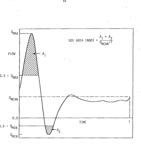
The dis.tribution of the area under the flow curve provides another measure of pulsatility. A 50% area index can be defined as the ratio of·

the area under the mean flow rate. Figure 1 illustrates graphically this definition. Area indices considered in this study were .the 50%, 70%, 80%, and 90% area indices. For a flat and dampened wavefo_rm, the .area i~dex will be greater than for a pulsatile waveform with sharp

peaks provided that the mean flow rate is equal. Thus, an inverse damping factor based on the area indices when plotted versus arterial

length may also be .diagnostic of flow obstructions.

In summary, the eight different general pulsatility indices

50% AREA INDEX

=

Fl:OW

[image:34.577.58.531.51.538.2]

0. 5 •

QMAX

PHYSIOLOGICAL MODEL

Raines et al. (1974) present a model 6f the human arterial tree from the iliac bi"furcation to the point where the popliteal artery meets the tibial branches. i:n my study, I retained the salient feature.s of

their model, especially the model geometry, but chose a different representation of ·the equation of state for numerical reasons. A schematic of the ~odel geometry is given in Figure 2.

The branches occurring in vivo along the total arterial section are lumped together into two model branches, the hypogastric artery and the profunda branch of the femoral artery. The peripheral beds of the

branches and the arterial tree distal from the popliteal artery are each accounted for by a lumped model conta·ining two flow resistances R1, R2 and one flow compliance C.

From measurements on arteriograms, Raines et al. (1974) obtained a relationship between the arterial area A(p0,x) at a reference pressure p0 and the distance x from the iliac bifurcation

A(p0,x) = 0.505exp(•0.192x0 ·5) O<= x <o:14 (21) 0.327exp(-0.0206x) 14<= x <=60

where xis measured in .cm and A in cm2 .

-jo.

06 m

~o

.14

m---l>+:l---~---o

.40 m---...i

ILIAC BIFURCATION COMMON FEMORAL ARTERY

SUPERFICIAL FEMORAL AND POPLITEAL ARTERY

HYPOGASTRIC

ARTERY

(RH ' RH ' CH)

₁

₂

DIRECTION. OF FLOW

PROFUNDA BRANCH

(Rp , Rp , Cp)

1 2

FIGURE 2. A Schematic of the Arteries in the Human Leg (pa and pv are the arterial and venous pressures,

DISTAL BEDS

(RD1' RDz' CD)

respectively, and _{(R1, R2, C) is a parameter}

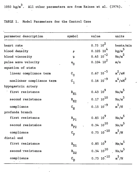
[image:36.782.89.721.63.532.2]

1050 kg/m3 . All other parameters are from Raines ·et al. (1974).

TABLE 1. Model Parameters for the Control Case

parameter description symbol value units

·heart rate 0.75 102 beats/min

blood density p 0.105 104 kg/m 3

blood viscosity µ 0.45 10-2 Ns/m 2

pulse wave velocity _ao 0.104 102 m/s equation of state

linear compliance term _co 0.67 10-5 m /sN 2 nonlin·ear compliance term _c1 0.16 10-9 m /sN 4 2 hyPogastric artery

first resistance _l1i1 0.43 109 Ns/m 5

second resistance _l1i2 0.17 1010 Ns/m 5

compliance _CH o .15 10-9 m5/N

profunda branch

first res·istante _RPl 0.85 109 Ns/m 5

second res-ista.Ilce _RP2 0.34 1010 Ns/m5

compliance _cP 0.75 10-10 m5/N

distal end

first resistance

Rui

0.85 109 Ns/m 5

second·resistance _11>2 0.34 1010 Ns/m 5

compliance _CD 0.75

10~

10 m5/N

To complete the mod.el, boundary values have to be specified at the proximal end of t·he artery. For thi,s purpose, I chose to use the

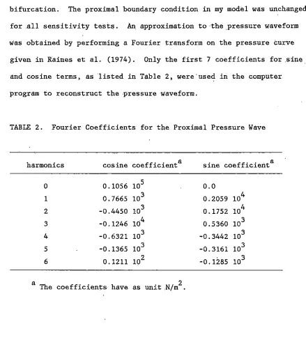
[image:37.571.49.495.70.632.2]

waveform by changes in the flow situations downstream from the iliac. bifurcation. The proximal boundary condition in my model was unchanged

for .all sensitivity tests. An approximation to ·the .Pressure waveform was obtained by performing a Fourier transform on the pressure curve

given in Raines et al. (1974). Only the first 7 coefficients for .sine and cosine terms, as 'listed in Table 2, were·used in the computer program to reconstruct the pressure waveform.

TABLE 2. Fourier Coefficients for the Proximal Pressure Wave

harmonics cosine coef f icienta sine coef f icienta

0 0.1056 105 0.0

1 0. 7665 103 0 .2059 104

2 -0.4450 103 0.1752 104

3 -0.1246 104 0.5360 103

4 -0.6321 103 -0.3442 103

5 -0.1365 103 -0. 3161 103

6 0 .1211 102 -0.1285 103

[image:38.571.51.490.101.602.2]

RESULTS AND DISCUSSION

Control Case

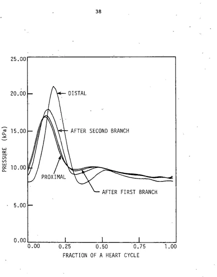
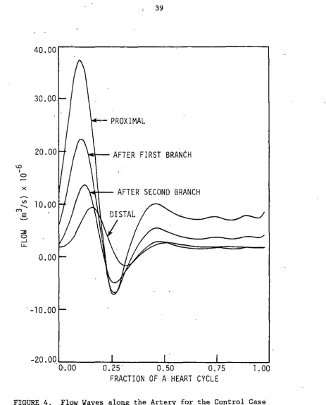
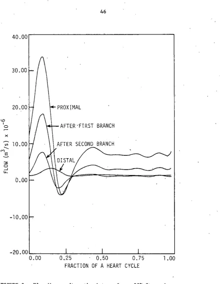
The control case is specified by the data given in Table 1 a.nd Figure 2. Figures 3 and 4 contain pressure and flow .waveforms;

respectively, at four different sites along the artery: at the proximal end, at .two 1ocations immediately following the branching points of the

hypogastric artery (first branch) and the profunda artery (second branch), and at the distal end.

The pressure wave travelling along the artery shows both an

amplification in the distal direction and the occurrence of a hump at the distal end, general:ly attributed to the effects of reflections. These findings are in good agreement with Raines et al. (1974); however,.

in my model the increase in. the pressure wave is more marked

corresponding favorably with data from physiological studies (Remington and Wood, 1956). This quantitatively different behavior is probably

caused by the different form of the equation of state in my model. The flow waveform exhibits a decrease in the distal direction as the .mean flow reduces after each branch. A phase of flow reversal occurs along the total arterial section. The mean flow rates are slightly higher than those given in Raines et al. (1974).

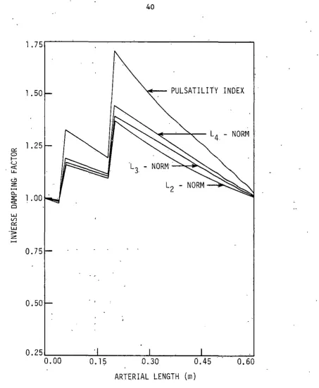
Figure 5 shows the inverse damping factors (IDF) of the pulsatility

index (PI) and of the L2, L3, and L4 norms. The IDF is defined as the ratio of a dis.tal index measurement to a proximal measurement. In the

5, the proximal measurement site remains fixed at the iliac bifurcation, and the distal measurement site varies along the artery. Note in Figure 5, that the IDF of the PI remains clearly above 0.67, a value which has been correlated with arterial disease by Baird et al. (1979). Instead of the IDF, Baird et al. (1979) use the damping factor which is found to

be greater than 1.5 for arteries with more than 50% stenosis; As shown in Figure S, branching causes an increase in the IDF as the reduction in

niean flow exceeds the reduction in the difference between .maximal and minimal flow rates (compare the definition of the pulsatility index}.

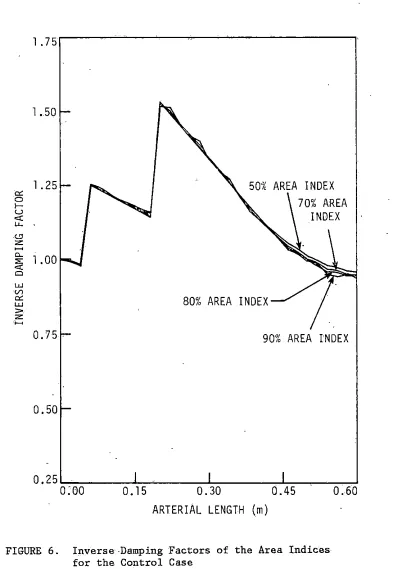
The IDFs for. the area indices are depicted in Figure 6. As is. the

case for the IDF of the pulsatility index, the IDFs of the area indices increase at branchi~g points _and decrease slowly along the normal

arterial sections". The ·graphs of the IDFs for all area indices are almost identical showing only small variations at the distal end which could be caused by numerical errors. At the present time, I do not have

a pertinent hemodynamic interpretation for this unexpected behavior. A linear model version, which excluded the nonlinear convective acceleration term of the momentum equation and the nonlinear term of the equation of state, shows different results. The pressure pulse wave is

not amplified in the distal direction, and the hump in the pressure

curve is less obviotis. However, if the convective acceleration term is

retained and a linear equation of state is used, both phenomena

25.00

20.00

"' 15.

00

"'-.,,,.

LU

""

::::r

(/")

(/")

"-'

"" 10. 00

"'-. 5 "'-.00

AFTER SECOND BRANCH

AFTER FIRST BRANCH

FRACTION OF A HEART CYCLE

[image:41.570.74.508.32.586.2]

40.00

30.00

PROXIMAL

20.00

_{AFTER FIRST BRANCH}

<.D I

0

x

_{AFTER SECOND. BRANCH}

"'

10.00

..._

M

E

~

3 0

--'

LI;.

0.00

-10.00

-20 .00 .___ ___

___._ ____

..._ ___

_._ ___

__.

·o,oo

0.25·

o.50

o.75

·1,00

FRACTION

OF

A HEART CYCLE

[image:42.575.49.512.41.616.2]

l. 75

l.50 "<+-

PULSATILITY INDEX

L4 -

NORM

""

l.25

0

I-_u

L3 <"(

w... 0

z:

~

a..

:.: <"( Cl LU V1

""

LU

-,,.

_z:

~

0.75

0.50

O.

l~

0 .. 30

0.45

ARTERIAL LENGTH

(m)

FIGURE 5.. Inverse Damping Factors of the Pulsatility Index

[image:43.571.59.513.40.591.2]

1. 75

l • .50

1.25

er: ₀

70% AREA

...

u

_INDEX

<:(

u..

.<.!:J

z

~ "-

_l.00

::;;:

<:( Cl

w

V)

""

80% AREA INDEX

w

>

z:

>--<

0. 75 .

_{90% AREA INDEX}

0.50

0. 25

.,_,.,-=----~~---'---''--~---.-I

_o:oo

_0.15

_0.30

_0.45

_0.60

ARTERIAL LENGTH

(m)

[image:44.571.61.470.59.628.2]

did not investigate the effects of elastic taper and possible changes in

the state of the peripher~l beds on the pressure waveform.

In summary, I concluded that the nonlinear model shows features not present in a linear model, since the convect.ive acceleration term in the

momentum equation appears. ·to be a significant factor in determining the pressure pulse wave behavior in both a straight and a tapered elastic

tube.

Sensitivity Analysis

With the control case as basis, a sensitivity analysis .was

conducted by investigating the influences of fluid properties,

properties of the arterial wall, branching, and distal resistance on the different generai pulsatility indices.

Changes in the blood density by 1% did not bring about significant changes in the. Pis. Similarly, setting the blood viscosity to 0,

thereby neglecting the friction term in the momentum equation, also had no significant effect. However, an increase of viscosity to 1.2 10 -2

2 .

Ns/m ,. which corresponds to a hematocrit of 70%, dampened the curves of the Pis and brought them close to values indicative of pathological·

situations.

The values of E , the pressure s-train modulus, given in Mozersky et

p ' .

al. (1972) served as primary data to study the influence of properties of the arterial wall. For this simulation, an approximation of (6) by the second order Taylor polynomial was used as an equation of state.

the arterial wall. For the E values of three different age groups, the _p corresponding PI curves show only slight differences and fall well into

the range- considered to be normal. Therefore, the stiffness of arterial walls seems to be only of minor importance in determining the PI

behavior.

-To· assess the effects- of branches, I simulated the occlusion of both model branches by increasing the four resistance values ten times.

Naturally, the steep rise occurring· at the ·branching points in the control case disappeared, but at the same time the rate of decrease

along normal arterial section was reduced. However, the drop in the IDF values was large enough to bring the curve of the pulsatility index below the threshold of 0.67 which is correlated with the occurrence of stenotic obstructions. Therefore,- low IDF values can also be indicative of reduced blood flow through the branches.

Changes in the distal resistance by factors of 2 and 0.5 brought

about significant variations in the Pis, but·did not shift the curves to low values that might be correlated with pathological situations.

Doubling the distal peripheral resistance resulted in very large rises

of the IDF across the two branching points and also in increased curve slopes. Decreasing the peripheral resistance to half the value of the control case diminishes the step size of the IDF across the branching

points and also diminishes the curve slopes.

Therefore, dislocating the probe by several centimeters should not result in significantly different measurements if the IDF method is to be of practical value: Except for the case of an increased peripheral

resistance', the rate of cha.nge in the distal reg:>on, away from branches, is small enough so that results obtained at two locations only

centimeters apart cqrrelate very closely.

Stenosed Arteries

To investigate the effect of obstructions, stenoses with different

degrees of occlusion were placed into the main artery 0 ,4m ·from th.e iliac bifurcation.

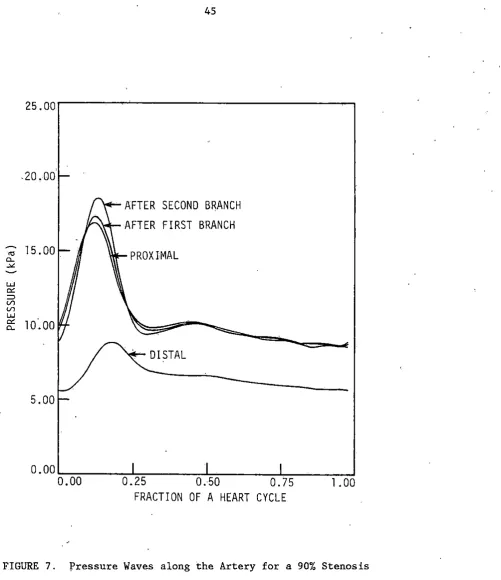
Figures 7 to 10 show the results for the case of an obstruction which provides a 90% lumen area reduction,. A large pressure dtop occur_s across the stenosis, so that the distal·pressure is very low. Also, the flow waveform distal to the stenosis is dampened and does not exhibit a

phase of flow reversal. The IDFs for the pulsatility index and the

1 _n -riorms drop very suddenly in the vicinity of the stenosis and stay

approximately constant downstream of the stenosis. Also, the IDFs for

the area indices ar.e ~hifted to lower values and differ significantly from the control case.

In summa.ry, the hemodynamic effects of a 90% stenosis are severe

and recognizable in the IDFs of all pulsatility indices considered. Therefore, a diagnosis of stencitic obstructions seems to ·be feasible for a severely occluded artery.

-20 .OD

AFTER SECOND BRANCH

AFTER FIRST BRANCH

"'

15.00

PROXIMAL

"--

-"'-w

°'

=>

(/) (/)

:;' w

°'

10.00

"--DISTAL

:::-5.00

O.DD~:-:--~~....,...'"="="~~~--''--~~~---1.~~~~-'

0.00

0.25

0.50

0.75

1.00

FRACTION OF A HEART CYCLE

[image:48.569.60.562.43.624.2]

40.00

30.00

20.00.

PROX!MAL

"'

I

AFTE.R ·FIRST BRANCH

0

~

x

[image:49.570.61.509.30.607.2]

"'

l 0. 00

AFTER SECOND B.RANCH

...

M

E ~.

3 0

-'

"'-b.00

-10.00

-2Q.00-~--~~---~---~

0.00 0.25 - 0.50 0.75 l.00

FRACTION OF A HEART CYCLE

1.

75

1.

50

1.25

""

0

f-u

<

u...

"'

z:

~ "-_::;;:

_1.00

< _Cl

w

Vl

""

w

>

z:

~

o.

75

L4 - NORM

0.50

PULSATILITY INDEX

90% STENOSIS

\

0. 25 .._ ___ __.. ____ _._ __ __._..._ ___ __,

0.00

0.15

0.30

0.45

0.60

ARTERIAL LENGTH

(m)

[image:50.573.74.428.50.581.2]

1 . 75 .

1.50

"" 1.25

0

f--u

L2

"'

z:

-a.

::;:

1

.00

;3

w

<./)

""

w > _z:

-

0.75

0.50

50% AREA INDEX

INDEX

90% AREA INDEX

90% STENOSIS

I

0.25'--...,.-~~...i.,-~~~-L.~~--L---''--~~--=-:!

0.00

0.15

0.30

0.45

0.60

ARTERIAL LENGTH

(m)

[image:51.571.70.524.49.613.2]

contain the data curves obtained for a

75%

stenosis. Still, the distal pressure ·is reduced, and the distal flow wave is dampened, but compared

to the

90%

stenosis, these effects are less pronounced. The drop in the IDF of the pulsatility index is also present; however, it takes place more slowly and continues also after the stenosis location. Therefore,

different results will be obtained at different measurement sites downstream of the stenosis. The more distal from the stenosis the

waveform is evaluated; the more indicative of an obstruction it will be.

Thus, from the model results it follows that less severe stenoses are best detected if the distal PI measurement is taken at some distance distal from the stenosis. Moreover it is important that measurements are not t~ken in the vicinity of.branches since big fluctuation of the·

PI occur around branches. For practical purposes, these two requirements are probably hard to meet, as the exact location of stenosis and branches are generally not known.

Evans et· al. (1980) indicate that in experimental animaI.s the state of the peripheral beds play an important role in determining the IDF for

nonsevere stenoses

(<86%).

To clarify this point, I placed a

50%

stenosis into my model and let the resistances of the peripheral bed vary by a factor of 2. For an increased peripheral resistance, the IDF

curves remain above 1, and are not significantly different from curves without a steno~is. However, if the distal resistance was decreased,

.the drop in the IDF was large enough to bring the IDF of the PI below

0.67

at the distal end_. A stenosis would then be diagnosed correctly.

Thus, an high peripheral resistance tends to cover the effects of

25.00

20.00

"' 15.0Q

0..

-"'

UJ

""

::::> (/") (/")

UJ

::;:: 10.00

5.00

. AFTER SECOND BRANCH

h'<Cr-AFTER FIRST BRANCH

PROXIMAL

0.25

0.50

0.75

~RACTION

OF A HEART CYCLE

1.00

40.00

30.00

PHOXIMAL

20.00

AFTER FIRST BRANCH

<D I

0

x

AFTER SECOND BRANCH

~

10.00

"'

'

M

E

3

0

-'

.u..

0.00

-10.00

-20 .00

...._~

__

___.. ____

..._ __

~_..._

___

__,

0.00

0.25

0.50

0.75

l.00

FRACTION OF A HEART CYCLE

[image:54.570.73.462.50.583.2]

l. 75

l . 50

PULSATILITY INDEX

l.

25

_L4-NORM

°"

_L3-NORM

0

t-u

«: .

u..

"'

z:

o._ l . 00 . ::;::

«: _Cl

w

V1

er:

w

:> _z:

~

0. 75

0.50 _{75?.; STENOS! S}

I

0.25~·~~~~-'-~~~~-'--~~---'~..___~~~--'

o.oo ·

o·.15

o.30

o.45

0.60

ARTERIAL LENGTH (m)

FIGURE 13. ·Inv~rse Damping ·Factors of the Pulsatility Index

[image:55.573.66.473.75.639.2]

1.75

1.50

l.25

0:: 0

I-'-'

c(

LL.

<.!l ~0% AREA INDEX

z

~

l.00 _{70% AREA}

Cl.

:::E:

c(

INDEX Cl

w

V1

0:: _{90% AREA INDEX}

w

:> _z

'~

0.75

_soi;

AREA INDEX

0.50

75% STENOS IS

I

0 . 2 5

"---:,----:-':-=---::-~----"-:::-'7=----;;--:=:::

b . 00 0. 1 5 0 . 30 0. 4 5 0 . 60

ARTERIAL LENGTH (m)

[image:56.577.69.500.58.603.2]

'

stenoses which are not severly constricting the arterial lumen.

From the model results, I concluded that (1) a low peripheral resistance is essential to allow the diagnosis of less severe stenoses with the PI method, and· (2) the eight general pulsatility indices in alr

situations show the same qualitative behavior, with the pulsatility index being the most sensitive index. Therefore, in a diagnostic method it should be sufficient to concentrate on the behavior of the