New Sampling Points for the 8 Node Brick Element for The Evaluation of Stiffness Matrix

(1)



Abstract: Calculation of the element stiffness matrix requires more computational effort because of handling large varying data. A new set of sampling points for the evaluation of 8 - node brick elements is introduced in this research study. A new set of integration points is a mimic of Gauss numerical integration method. The proposed set of sampling points is evaluated using the standard problems and compared with conventional Gauss numerical integration method and found that CPU execution time considerably reduced for the analysis of brick elements without compromising in the convergence rate, efficiency in the results and accuracy of values.

Keywords: Quadrature, Stiffness Matrix, Brick Elements, Integration Points.

I. INTRODUCTION

Finite element analysis (FEA) is an approach used to compute problems in engineering. For the cases of realistic problems, we use three dimensional elements for solving problems in FEM. Calculation the element stiffness matrix requires more computational effort because of handling large varying data. The requirement of finite element analysis is increasing day by day because of necessity in analyzing larger structures with higher degrees of freedom. Computation of mass matrix requires more precision because of calculating large varying data thus number of points for the integration in stiffness matrix calculation plays a significant role in the precision of results [1]. During the calculation of stiffness matrix, it is found that for one-point quadrature the results found to be getting in singular matrix thus it will lead to stability issues Dan et al. has proposed a new method to remove this singularity in one-point quadrature [2]. A group super matrix procedure was developed by G. Zlokoviet.al for the derivation of element stiffness matrices of brick elements and quadrilateral and also in G-invariant subspaces introduced monomial shape functions [3]. The typical 8 node brick element is shown in figure 1 and it has 8 nodes with 24 degrees of freedom.Jeonget.al had modified the conventional gauss sampling points of 16 node and 6 node elements and tested successfully on beams at various conditions [4]. Shmuel L. weissman formulated low order brick elements of high accuracy with the principle of three-field variational principle [5]. A simple 5-point integration scheme for quadrilateral element was developed by Shengrong Huet.al

[6]. A stable midpoint quadrature for the quadrilateral

Revised Manuscript Received on April 07, 2019.

Shyjo Johnson, Research Scholar, Department of Mechanical Engineering, Hindustan Institute of Technology & Science, Padur, Chennai Dr. T. Jeyapoovan, Professor, Department of Mechanical Engineering, Hindustan Institute of Technology & Science, Padur, Chennai

element was proposed by Jeyakarthikeyan P.V.et.al [7]. In this paper we propose a new set of sampling points for the Calculation of the global stiffness matrix for the 8 node brick element and the convergence study of 8 node brick element on comparison with gauss quadrature is done.

II. NUMERICAL INTEGRATION

Numerical integration is the important method for evaluating integrals over the brick elements. For general case of finite elements, the expressions for the integration of load vectors and element stiffness matrices cannot be done analytically. Instead of that load vectors and element stiffness matrices are evaluated by using some integration rule numerically. For estimation of element matrices and vectors usually we use numerical integration methods for different types of finite elements. Gauss numerical integration is an approximation of the definite integral of a function and can be stated within the domain of integration as the weighted sum of functional values at points specified. While calculating element stiffness matrix for the brick elements a lot of effort has to be taken. This paper presents a study on numerical integration methods for 8-noded brick elements. Numerical integration of brick elements is done by Gauss numerical integration methods. A new set of integration points is introduced in this paper which is a mimic of gauss numerical integration method. The sampling points for new method are on the corner points and face centers. The fourteen-point integration method is tested using eight node brick element with few problems.

(a)

New Sampling Points for the 8 -Node Brick

Element for The Evaluation of Stiffness Matrix

(2)

(b)

Fig.1: (a) 14-point sampling method (b) Gauss 3-point quadrature

A. Derivation of new set of points

For the purpose of deriving the new set of points, undetermined coefficients method is used. The main aim is to determine a new set of sampling points and weights. The typical brick is considered with an interior cube where 14 sampling locations were chosen. Eight points are assumed to be located at the corners of the cube and six sampling points are assumed to be located at the axis of the cube. Fig.1 (a) shows the assumed new set of sampling points and Fig.1 (b) shows the gauss 3-point quadrature sampling point locations. Each sampling point has for unknowns and they are the weights and coordinates so there will be 56 unknowns for the new set of sampling points. In order to integrate at the same time reducing the error in calculation, a polynomial should be chosen and it should contain the terms in r, s and t. Based on the above assumptions we have a total of four unknowns they are the weights and the points, namely a, Wa, b and Wb. The following polynomial is assumed to integrate

 

,

2

...

7 2 6 2 5 4 3 2

1







r

s

t

a

r

a

s

a

t

a

r

a

s

a

t

(1) On integrating (1) we get the following equation

  

  







1 1 1 1 1 1 2 5 4 3 2 1

....

)

,

(

r

s

t

drdsdt

a

r

a

s

a

t

a

r

(2) on performing the numerical integration on (2) we get

 

...

3

8

3

8

3

8

₅ ₆ ₇

1















































a

(3)

Evaluation of the function



can be done by using the following numerical form



r

s

t



W

i

,

14 1 1









 ₍₄₎

Again substituting (1) in (4) we get

[image:2.595.129.237.61.171.2] [image:2.595.362.461.62.154.2] [image:2.595.303.561.201.361.2] [image:2.595.302.550.419.613.2]











...



.... ... ... ... 4 3 2 1 14 4 3 2 1 2 4 3 2 1 1                 t a s a r a a W t a s a r a a W t a s a r a a W

..

...

)

.

...

.

(

)

.

...

.

(

)

.

...

.

(

3 14 3 2 1 2 14 3 2 1 1 14 3 2 1





a

W

a

W

a

W

(5) Based on the locations of sampling points shown in Fig. 1 (a) there can be only two weights Wa and Wb. For each integration points, the coordinates and the weights are substituted simultaneously and simplifying we get a set of simultaneous equations as the follows.

9 8 8 5 8 2 8 3 8 2 8 8 6 8 4 4 4 2 2        a b a b a b a W a W b W a W b W a W W (6) On substituting the points and solving the (6) the set of points are found and shown in table I. For three dimensional brick element the reduced integration will be









i

i i

i

s

t

W

r

f

drdsdt

t

s

r

f

I

  



   



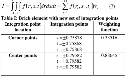
14 1 1 1 1 1 1 1

,

(7)

Table I: Brick element with new set of integration points Integration point

location

Integration points Weighting function Corner points s =±0.75878

t =±0.75868 r =±0.75868

0.33516

Center points s =±0.79582 t =±0.79582 r =±0.79582

0.88645

III. ELEMENT STIFFNESS MATRIX FOR THE BRICK ELEMENTS.

Strain energy (U) can be defined as



u

v

w

  

K

u

v

w



dv

U

T v T

2

1

2

1 _



_





(8)

 









































2

1

0

2

1

0

2

1

0

1

0

1

0

1

2

1

1 







E

zx yz xy zz yy xx (9)

 





 

D

 



(10)

The material matrix (D) can be defined as a function of Poisson’s ratio (μ) and Young’s modulus (E). In the formulation of stiffness matrix for brick elements the function for defining the material functions (E and μ), field geometry defining functions (x, y and z) and variable defining function (u, v and w) are described in (11).

i i n i

u

t

s

r

N

u

(

)

1





_i _i

n i

v

t

s

r

N

v

(

)

1





i i n i

w

t

s

r

N

w

(

)

1



(3)

i i n i

x

t

s

r

N

x

(

)

1





_i _i

n i

y

t

s

r

N

y

(

)

1





i i n i

z

t

s

r

N

z

(

)

1





i i n i

E

t

s

r

N

E

(

)

1





i i

n i

t

s

r

N



(

)

1





(11)

In order to have unique mapping of elements, there should be only one set of Cartesian coordinates for each set of corresponding non-dimensional coordinates. Jacobian matrix is used for this mapping of elements and it will be

















t

z

t

y

t

x

s

z

s

y

s

x

r

z

r

y

r

x

J

(12)

The general strain equation is

 



































































z

u

x

w

y

w

z

v

x

v

y

u

z

w

y

v

x

u

zx yz xy zz yy xx





(13)

 

 





T

w

v

u

B

*





(14) Where [B] is the strain displacement matrix which can be defined in terms of plane strain and plane stress as shown in (15)

 

B

63n



     

B

169



B

2 99



B

3 93n (15)



 



T

n n n T

w

v

u

w

v

u

w

v

u

w

v

u



1 1 1 2 2 2

.

₍₁₆₎

Where ‘n’ is defined as nodes per element

 















0

1

0

1

0

1

0

1

0

1

0

1

0

1

0

1

0

1

B

 

                             33 32 31 23 22 21 13 12 11 33 32 31 23 22 21 13 12 11 33 32 31 23 22 21 13 12 11 2 0 0 0 0 0 0 0 0 0 0 0 0 0 0 0 0 0 0 0 0 0 0 0 0 0 0 0 0 0 0 0 0 0 0 0 0 0 0 0 0 0 0 0 0 0 0 0 0 0 0 0 0 0 0 JI JI JI JI JI JI JI JI JI JI JI JI JI JI JI JI JI JI JI JI JI JI JI JI JI JI JI B                                                                                                        . 0 0 . . . 0 0 0 0 0 0 . . . 0 0 0 0 0 0 . . . 0 0 0 0 0 0 . . . 0 0 0 0 0 0 . . . 0 0 0 0 0 0 . . . 0 0 0 0 0 0 . . . 0 0 0 0 0 0 . . . 0 0 0 0 0 0 . . . 0 0 0 0 2 1 2 1 2 1 2 1 2 1 2 1 2 1 2 1 2 1 3 t N t N t N s N s N s N r N r N r N t N t N t N s N s N s N r N r N r N t N t N t N s N s N s N r N r N r N B n n n n n n n n n (17) The element stiffness matrix for brick element can be written as

 

K

e 1



B

e



r

,

s

,

t





T



D

e



r

,

s

,

t







B

e



r

,

s

,

t



  

det

J

e

drdsdt

1 1 1 1 1

  

  



(18) Suitable numerical quadrature can be defined following equation.

 

K

W

_j

W

_k

K

e



r

_i

s

_j

t

_k



drdsdt

P i Q j R k i e

,

1 1 1



  



(19)

Here P, Q and R represents the sampling points number along the r, s and t directions and Wi, Wj, Wk represents the sampling weights for the respective Quadrature.

IV. NUMERICALRESULTS

Finite element analysis (FEA) is method of approximation thus it is validating the performance and efficiency of the new set of points. There are several studies which lead towards some pathological test to validate the results [8, 9].

A. Test for comparing the accuracy of sampling points Accuracy of results is an important factor in evaluation of stiffness matrix in finite element analysis. Wide ranges of problems are available for validating the results. A cantilever beam is chosen for the evaluation. The boundary and geometry conditions of cantilever beam are shown in Fig. 2. The cantilever beam is discretized into1464 brick elements and 2051 nodes as shown in fig. 3. An isotropic material with a property of linearly elastic is chosen with young’s modulus (E) of 200000 and Poisson’s ratio of 0.3. The cantilever beam is evaluated using the new set of points and conventional gauss sampling points

(4)

[image:4.595.52.280.46.154.2] [image:4.595.72.265.397.700.2]

Fig.2: Boundary and geometry conditions of cantilever beam

Fig. 3: Discretization of cantilever beam with 8 –node brick element

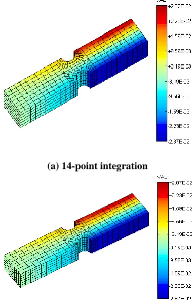
(a) 14-point integration

(b) Gauss 3x3x3 integration

Fig. 4: Nodal displacement along X direction

(a) 14-point integration

Fig. 5: Nodal displacement along Y direction

(5)

[image:5.595.81.279.52.212.2]

Fig. 6: Nodal displacement along Z direction The nodal displacement of the tested cantilever beam is plotted using MATLAB and shown in figure (4-6) along X, Y and Z directions. Table II shows the nodal displacement values along X, Y and Z direction for cantilever beam using proposed sampling points and Gauss quadrature. It is clear from the figure and table, the nodal displacement results of proposed sampling points and Gauss quadrature is found to be exactly same

B. Hour Glass stability test

Hourglass stability test is one of the important tests for any scheme of numerical integration. In this research work a numerical example defined by Hansbo [10] is used to verify the stability of finite elements. A unit cube is discretized into 1000 brick elements, 1331 nodes and 1331 x 3 degrees of freedom. An isotropic material with a property of linearly elastic is chosen with a Poisson’s ratio of 0.3 and young’s modulus of 1000. Unit cube is solved using the new set of sampling points and conventional gauss sampling points (3x3x3). It is found that there are instability issues found for the one-point quadrature which is shown in fig. 7(a) at the same time we can see that there are no stability issues for the proposed set of points and found that the new set of points shows exactly same surface texture shown in figure 7(b) and 7(c).

(a) . One-point gauss quadrature

(b) Gauss quadrature (3x3x3)

[image:5.595.63.289.540.686.2]

(c) 14-point method Fig.7: hour glass stability verification C. Convergence test

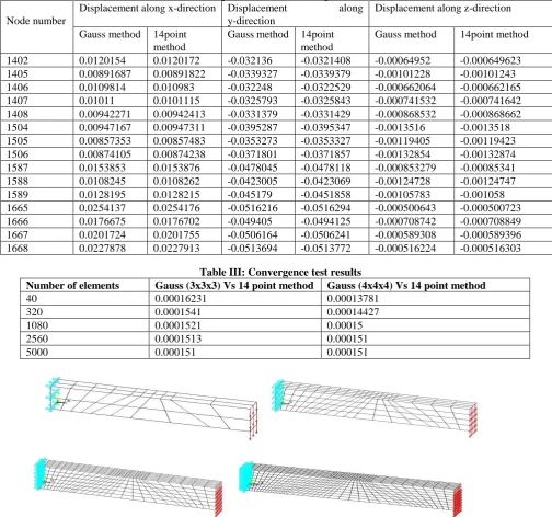
Many researchers have chosen this problem to validate the efficiency of the quadrature [11, 12]. The convergence test is conducted to determine the convergence of values obtained during the numerical integration. The convergence the displacement values are obtained from the (20). The convergence test is analyzed using distorted 8 node brick elements. The discretization of the convergence problem is shown in the fig.8. The results of the gauss sampling points and proposed sampling points converge with increasing the number of nodes. From the fig. 9 the general trend shown is initially the convergence rate is more on increasing the number of elements the convergence rate is getting decreased and it is found that the rate is getting to a constant value. Table III shows the displacement error values using gauss method and 14-point method.











 





n

j

Gauss i n

j

oposed i Gauss i

d

U

1

2 1

2 Pr

(6)

[image:6.595.41.546.71.543.2] [image:6.595.43.548.72.303.2]

Table II: Nodal displacement values along X, Y and Z direction Node number

Displacement along x-direction Displacement along y-direction

Displacement along z-direction

Gauss method 14point method

1402 0.0120154 0.0120172 -0.032136 -0.0321408 -0.00064952 -0.000649623

1405 0.00891687 0.00891822 -0.0339327 -0.0339379 -0.00101228 -0.00101243

1406 0.0109814 0.010983 -0.032248 -0.0322529 -0.000662064 -0.000662165

1407 0.01011 0.0101115 -0.0325793 -0.0325843 -0.000741532 -0.000741642

1408 0.00942271 0.00942413 -0.0331379 -0.0331429 -0.000868532 -0.000868662

1504 0.00947167 0.00947311 -0.0395287 -0.0395347 -0.0013516 -0.0013518

1505 0.00857353 0.00857483 -0.0353273 -0.0353327 -0.00119405 -0.00119423

1506 0.00874105 0.00874238 -0.0371801 -0.0371857 -0.00132854 -0.00132874

1587 0.0153853 0.0153876 -0.0478045 -0.0478118 -0.000853279 -0.00085341

1588 0.0108245 0.0108262 -0.0423005 -0.0423069 -0.00124728 -0.00124747

1589 0.0128195 0.0128215 -0.045179 -0.0451858 -0.00105783 -0.001058

1665 0.0254137 0.0254176 -0.0516216 -0.0516294 -0.000500643 -0.000500723

1666 0.0176675 0.0176702 -0.049405 -0.0494125 -0.000708742 -0.000708849

1667 0.0201724 0.0201755 -0.0506164 -0.0506241 -0.000589308 -0.000589396

1668 0.0227878 0.0227913 -0.0513694 -0.0513772 -0.000516224 -0.000516303

Table III: Convergence test results

Number of elements Gauss (3x3x3) Vs 14 point method Gauss (4x4x4) Vs 14 point method

40 0.00016231 0.00013781

320 0.0001541 0.00014427

1080 0.0001521 0.00015

2560 0.0001513 0.000151

5000 0.000151 0.000151

(7)

[image:7.595.73.286.51.176.2]

Table IV: Stiffness matrix error

Method error

Gauss (3x3x3) Vs 14-point method 0.0011

[image:7.595.311.576.54.148.2]

Gauss (4x4x4) Vs 14-point method 0.000996

Fig. 9: Convergence error plot D. Patch Test

The patch test for the brick elements is evaluated using standard problem [9] and patch test is conducted on the distorted elements as shown in fig. 11. A linear elastic material with Young’s modulus (E) of 1e06 and Poisson’s ratio (ϑ) of 0.25 is assumed. The main aim of conducting patch test is to assess the element stiffness matrices obtained by using different quadrature. The patch test is carried out to determine the error in stiffness matrix on comparison with standard one. The following equation is used to ensure the patch test for the brick elements.

Stiffness matrix error (



_s) is given by







   





_n

i n

j

Gauss ij n

i n

j

oposed ij Gauss ij

s

K

1 1 1 1

2 Pr



(21)

The patch test results are shown in Table IV. The results show that on comparing with Gauss integration points, the new set of integration points are found to be negligible so it can be stated that it had passed patch test.

Fig. 10: Discretization of 8- node brick element for the Patch Test

E. CPU time comparison test

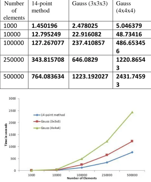
[image:7.595.302.550.330.629.2]

The computation of global stiffness matrix consists of calculation of large varying data thus it will lead to more computational time. The time needed for the calculation of global stiffness matrix for 8 node brick element is checked using gauss numerical integration method and new set of points using typical 8 nodded elements. For CPU time analysis, programs of the brick elements for Gauss points and new sampling points are written. The comparison is shown in Table V and fig. 11.

Table V: CPU execution time (Vs) number of elements Number

of elements

14-point method

Gauss (3x3x3) Gauss (4x4x4)

1000

1.450196

2.478025

5.046379

10000

12.795249

22.916082

48.73416

100000

127.267077 237.410857

486.65345

6 250000

343.815708 646.0829

1220.8654

3 500000

764.083634 1223.192027 2431.7459

[image:7.595.47.205.358.428.2]

3

Fig. 11: Time comparison for the evaluation of stiffness matrix

V. CONCLUSION

[image:7.595.106.244.489.652.2]

(8)

elements in finite element analysis. The method of formulation of sampling points is very direct and simple. The accuracy and efficiency of the brick elements is examined using several numerical standard example problems defined by many researchers. It includes hourglass stability control test and convergence test for the brick elements. The result shows that the proposed set of sampling points gives accurate results on various tests. Based on the study the following conclusions are inferred:

 The proposed set of points considerably reduced the CPU execution time for the analysis of brick elements without compromising in the convergence rate, efficiency in the results and accuracy of values.

 The proposed set of points significantly pertains the results with same accuracy and convergence rate on comparison with conventional gauss quadrature method

 The CPU execution time of proposed set of points for the evaluation of global stiffness matrix is found to be reduced to almost half of the execution time taken by the gauss quadrature method.

 Significantly, the proposed method can also handle distorted brick elements because from the patch test results shows that the error is found to be too less thus we can infer that complex problems can be solved using the new set of points.

 The overall displacement results show that the proposed sampling points produce exactly same results on comparing with the existing gauss numerical quadrature method.

REFERENCE

1. Eli Hanukah, SefiGivli. Improving mass matrix and inverse mass matrix computations of hexahedral elements. Finite Elements in Analysis and Design 2018; 144:1–14.

2. Dan Kosloff, Gerald A. Frazier. Treatment of hourglass patterns in low order finite element codes. International journal for numerical and analytical methods in geomechanics.1978; 2: 57-72.

3. G.Zlokovi, T. Maneski, M. Nestorovi. Group theoretical formulation of quadrilateral and hexahedral isoparametric finite elements. Computers andStructures.2004;82: 883–899.

4. Jeong Oun Kim, Young-Doo Kwon. On the modification of gauss sampling points of 6-node and 16-node isoparametric finite elements. Computers & Structures. 1997;63 (3): 607-623.

5. Shmuel L.Weissman. High accuracy low order three dimensional brick elements. International journal for numerical methods in engineering.1996; 39: 2337-2361.

6. Shengrong Hu, Jingjing Xu, Xinhong Liu, Murong Yan. A simple and robust quadrilateral non-conforming element with a special 5-point quadrature. 2018; 69:71-77.

7. Jeyakarthikeyan P.V., Subramanian G., Yogeshwaran R. An alternate stable midpoint quadrature to improve the element stiffness matrix of quadrilaterals for application of functionally graded materials (FGM). Computers and Structures.2017;178:71-87.

8. R.H Macneal, Robert L Harder. A proposed standard set of problem to test finite element accuracy. Finite element analysis and design. 1985; 1:3-20.

9. K Mallikarjuna Rao, U Shrinivasaa. Set of pathological tests to validate new finite elements. Sadhana. 2001; 26(6): 549–590.

10. Peter Hansbo. A new approach to quadrature for finite elements incorporating hourglass control as a special case, Computer Methods in Applied Mechanics and Engineering.1998;8:301-309.

11. Rathod HT. Some analytical integration formulae for a four node isoparametric element. Computers & Structures. 1988; 30(5): 1101–1109.

12. Cheung YK, Zhang YX, Chen WJ. A refined non-conforming plane quadrilateral element. Computers & Structures 2000;78(5):699–709. 13. A. J. M. Ferreira, MATLAB codes for finite element analysis. 1st

edition: Springer Netherlands; 2009.