519 | P a g e
FORECASTING PROFITABILITY IN EQUITY
TRADES USING RANDOM FOREST, SUPPORT
VECTOR MACHINE AND XGBOOST
Ritesh Ghosh
1, Priyanka Purkayastha
21
Engineer, Cisco Video Technologies India Pvt Ltd, (India)
2
Lead Consultant, BT e-Serv India Pvt Ltd, (India)
ABSTRACT
There has been enormous number of research on applying machine learning to forecast direct price value as well as direction of equity and derivative instruments in stock markets worldwide. Many of the proposed models also considers the effect of transaction costs, which is an important factor for intraday trading. Most of the models examines the forecasting of price or direction of the underlying instrument only in the next time unit. Considering stock market instrument’s underlying values as time series data points, predicting the value or direction for only the immediate data point is not justified. There has been also a lack of studies inspecting the predictability of profit over transaction costs for certain time durations ahead. This experimental research tries to predict the profitability over and above the transaction cost within the window of next few time units for an equity instrument traded in National Stock Exchange in India. The underlying machine learning approaches used to perform the experiment are non-linear supervised algorithms like Random Forest, Support Vector Machine and Extreme Gradient Boosting (xgboost). Extensive research has been made to derive the independent variables to perform the experiment from direct price data points of underlying equity instrument. The experimental research suggests that xgboost algorithm outperforms the other classification methods in terms of predicting the profitability from trading of the underlying instrument.
Keywords: Derivatives, Equity, Extreme Gradient Boosting, Forecasting, Profitability, Random
Forest, Stock market, Support Vector Machine
I. INTRODUCTION
Intraday trading in various stock market instruments is very popular method of trading in major stock exchanges
around the world mostly because of few reasons such as profit within short span of time, minimal effect of
economic factors, possibility of both long and short positions etc. Since, speed is a challenging factor to decide
the position to be taken, most of the intraday trades placed in the exchanges these days are machine trades i.e.
computers decide the trade to be taken. Underlying algorithms to machine trades require to be intelligent enough
to make accumulated profits over long run. Hence, being able to accurately forecast the trades is significant to
researchers worldwide.
The prediction of any tradable instrument is complex due to the inherent nature of financial time series
consisting noise and non-stationarity. Noise refers to the serially uncorrelated random variables with zero mean
520 | P a g e
with respect to the present data point. The nonstationary refers to the constant change in mean and variance of
the time series data. Change in value of any tradable instrument occurs due to uncountable factors such as
sentiment of traders, reaction of participating algorithms, economic or political change etc. Henceforth,
predicting the profitability of any tradable instrument in stock exchange is extremely difficult.
Leung et al., 2000[1] experimented with various classification models like logit, LDA and neural network, but
these models predict the direction of few globally traded market indices. Kamruzzaman and Sarkar, 2004[2]
experimented with various technical indicators to predict currency instrument rates using neural networks, but
this model tries to predict continuous value of the underlying instrument.
Even though there exist many literatures to predict the price or direction of any tradable instrument, price or
direction cannot be accurately predicted for the immediate next time period due to enormous number of factors
involved in change of the price. Since the fact is that different traders and algorithms employ different strategies
to trade any instrument, conducting an empirical study is important to analyze the behavior of price over next
few time periods instead of restricting to next. Also, predicting direction of underlying instrument not
necessarily accounts to profitability, almost certainly not when the chosen forecasting period is restricted to the
immediate next period. Thus, there seems to exist a gap in existing literatures to analyze the predictability of
profit in intraday financial time series considering the transaction costs and forecasting period.
The proposed experiment study realizes the rapid growth of algorithmic trades in Indian stock market and tries
to accurately predict the profitability of intraday applying non-linear classification techniques in intraday
financial time series.
II. LITERATURE REVIEW
In recent times, a growing number of experiments have been performed considering the trend of instruments
traded in stock markets e.g. O’ Connor, Remus and Griggs, 1997[3], Wu and Zhang, 1997[4]. These days, many
foreign institutional investors are more attracted towards developing markets. According to Harvey, 1995[5]
developing markets contain more regional information than developed markets; thus, predicting developing
markets are comparatively less complex than developed markets.
In accordance to prior research e.g. Van and Robert, 1997[6], Cheng et al., 1996[7], artificial neural networks
(ANN) was very successful to model stock market instrument’s time series data. Even though ANN can model
complex time series data to an extent, it has some limitations with respect to predicting stock market time series
data such as it tends to over fit noise and multi dimensionality which exists in financial time series data, mostly
because ANN tries to fall into the local optimal solution. Also, ANN is very inefficient to get trained and predict
within a short span of time. Considering, the intraday time periods such as one minute, two minutes, five
minutes, ANN would not be very efficient in practical implementation. Thus, the proposed experimental
research does not consider ANN for modelling.
Over last two decades, there has been an increase in experimentation using Support Vector Machines (SVM) to
model financial time series e.g. Kim, 2003[8], Tay and Cao, 2001[9]. SVM methodology was first formulated by
Vapnik and team in 1997[10]. While experimenting, it has been observed that SVM is more efficient with respect
to time taken to forecast than ANN.
A little younger technique than SVM named Random Forest was invented by Breiman in 2001[11]. It has also
521 | P a g e
Creamer and Freund, 2004[13]. Random forest ideology has been originated from the decision tree methodology,
where it tries to choose the best decision tree out of the multiple decision tree models formed from the data.
Both random forest and support vector machines try to fit the given data with multiple independent variables
irrespective of the underlying distribution of data and tend toward global optimum, thus occurrence of over
fitting is unlikely.
An extremely new machine learning technique known as Extreme Gradient Boosting (Xgboost) is applied to
solve multiple machine learning problems in diverse domains. The underlying method employs traditional
Gradient Boosting machine learning techniques. It was initially started as a research project by Tianqi Chen and
Carlos Guestrin[14] as part of Distributed (Deep) Machine Learning Community (DMLC) group, whereas the
first version has been released on early 2014. The major benefit of Xgboost is that it supports distributed
processing environments like Apach Spark and Apach Hadoop, which are being used widely in big data
analytics research areas.
Thus, the proposed experimental research considers SVM, Random Forest and Xgboost to model the underlying
instrument’s time series data. This research does not consider Decision tree and Gradient Boosting because
Random Forest takes into consideration the effect of Decision Trees on data and Xgboost is based on the
original model of Gradient Boosting.
III. INDENTATIONS AND EQUATIONS
In this sections the applied machine learning techniques of SVM, Rand Forest and Xgboost have been discussed
in detail with brief mathematical equations.
3.1. Support Vector Machine (SVM)
The original SVM algorithm was introduced to model linear relationship in data. The methodology for which is
formulated as below.
Given a dataset of n data points of the form
(x
1, y
1), …., (x
n, y
n).
Where
x
i is a vector of any dimension known as independent variable andy
i is either 0 or 1 (either factor orinteger data point) indicating the class to which
x
i belongs to known as dependent variable.A maximum margin hyperplane is established to divide the group of data points
x
i for whichy
i = 1 from thegroup of data points
x
i for whichy
i = 0, such that distance between the hyperplane and nearest data point ofx
ifrom either group is maximized.
The hyperplane can be formulated by approximating the following function:
y = f(x) = w.ϕ(x) - b
Where
ϕ(x)
is the high dimensional feature space and is non-linearly mapped from the input spacex
. The coefficientsw
andb
are estimated by minimizing following function:[C/n.∑max(0, 1 – y
i(w.ϕ(x) - b))] + λ/2||w||
2522 | P a g e
ensuring
x
i lies on the correct size of the margin. Here, the term[C/n.∑max(0, 1 – y
i(w.ϕ(x) - b))]
isempirical error (risk) and the term
λ/2||w||
2is called regularized term.C
is a regularization constant which determines the trade-off between the empirical error term and the regularized term.Stock market time series data is non-linear in nature. To solve such kind of a problem, Vapnik (the inventor of
the methodology) suggested to create non-linear classifiers by applying kernel trick to maximum margin
hyperplane. The formula remains same except that dot product of
w.ϕ(x)
is replaced by a non-linear kernel function.This research methodology uses Gaussian Radial Basis Function as the kernel trick where
K(x
i, x
j) = exp(-γ||x
i- x
j||
2)
forγ > 0
Per Tay and Cao, 2001, an effective SVM model can be obtained by proper selection of regularization constant
C
and the kernel parameterγ
, without which SVM may over fit or the under fit the data. This study experiments to find optimal values of the two mentioned parameters of SVM model using libsvm R library.3.2. Random Forest
In general, when Decision Trees are trained too deep, they tend over fit the training dataset with low bias and
high variance. Random Forest method tries to reduce the variance by training different parts of the same dataset
to average out the effect of multiple Decision Trees by applying the technique of Bagging. Bagging fits multiple
trees by repeatedly selecting a random sample with replacement from the training dataset and average out the
prediction result from the formed trees.
According to Breiman, 2001[12], first a random vector
V
k is created consisting of a number of independentrandom integers between 1 and
k
, this vector has to be independent of the past vectorsV
1, ..., V
k-1 but of thesame distribution; then a tree is created using the training set and the vector
V
k, which results to a classifier treeh(x, V
k)
wherex
is an input vector. Following the same approach many trees are created and the most popularclass is being voted by each tree for the most popular class at input
x
.Hence, an ensemble of classifier trees
h
1(x), h
2(x), ..., h
k(x)
are formed from the distribution of the randomvector
Y, X
. This defines the margin function as:f
margin(X, Y) = av
k.I(h
k(X) = Y)
Where
I(y)
is the indicator function. The margin indicates average number of votes for the right class exceeding the average number of votes for any other class. Confidence in the classification is directly proportional to themargin.
3.3. Extreme Gradient Boosting (Xgboost)
The underlying principle behind Xgboost is Gradient Boosting and Gradient Boosting itself relies heavily on
Gradient Descent.
3.3.1. Gradient Descent
Considering
x
being scalar, letf(x)
be the function to be minimized. One way to iteratively minimize and find the correspondingx
at the minima is to follow below update rule at thei
th iteration:523 | P a g e
Where
q
is a positive constant andx
(0) can be any arbitrary value. In effect, the value ofx
found in the current iteration is its value in the previous iteration added to some fraction of the gradient (slope) at the previous value.The iteration is stopped when
x
(i)= x
(i-1).In effect, every move is considered estimating an amount proportional to the gradient, because the gradient has
to gradually become 0 near the minima, and the gradient is higher farther away from minima. That is why longer
step iterations are taken when farther away from minima, whereas shorter steps are taken when nearer to
minima.
In similar fashion if
x
is a vector, the theory remains the same. Thus, for thei
th iteration and thej
th dimension, the update rule would be:x
(i)j= x
(i-1)j– q.df(x
(i-1)j)/dx
All dimensions are adjusted at every iteration i.e. the vector
x
itself is moved in a direction where each individual component minimizesf(x)
.3.3.2. Gradient Boosting
Gradient Boosting incorporates the technique of Gradient Descent in supervised learning i.e. a function
f(x)
is minimized. A loss functionL
is incorporated whose value increases when the classifier performance degrades. For Gradient Boosting loss functions, must be differentiable e.g. the squared error between the actual andpredicted value:
L
= (y
i– h(x
i))
2Hence,
f(x) = ∑
Ni=1L(y
i, h(x
i))
loss requires to be minimized for all points, whereh(x)
is the classifier andN
is the number of points. Therefore, as like gradient Descent, minimization requires to happen with respect toclassification function
h(x)
, because a predictor requires to be established that minimizes total lossf(x)
. The minimization is performed in multiple steps, where at every step a tree is added that emulates adding a gradientbased correction as like in GD. The
h(x)
after the most minimized step becomes the ultimate result, where the classification function exists as a bunch of trees and each tree represents the update in some iteration.3.3.3. Xgboost
Xgboost follows the same principle of gradient boosting but includes regression penalties in the boosting
equation. Xgboost uses a more regularized model formalization to control over-fitting but it also leverages the
structure of the underlying hardware to speed up computing times and facilitates memory usage, which are very
important resources to consider while performing computation of boosted tree algorithms. Thus, Xgboost
provides a better real time computational performance.
IV. EXPERIMENTAL RESULTS
4.1. Data Preparation
One of the major challenges faced while applying is the preparation of independent variables or predictor
variables. Choosing the proper set of independent variables is of utmost importance for accurate forecasting,
524 | P a g e
This study incorporates two different categories of data as independent variables, whose values are derived from
the Open
(O)
, High(H)
, Low(L)
and Close(C)
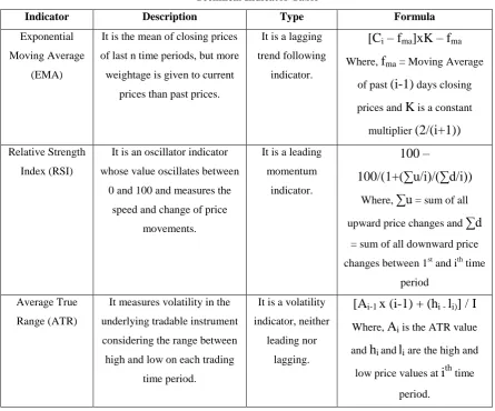
values of the underlying instrument for a specific time period.First category of independent variables includes three major types of technical indicators – Exponential Moving
Average
(MA)
, Relative Strength Index(RSI)
and Average True Range(ATR)
. Table 1 describes each of these indicators in details.Table 1
Technical Indicator Table
Indicator Description Type Formula
Exponential
Moving Average
(EMA)
It is the mean of closing prices
of last n time periods, but more
weightage is given to current
prices than past prices.
It is a lagging
trend following
indicator.
[C
i– f
ma]xK – f
maWhere,
f
ma = Moving Averageof past
(i-1)
days closing prices andK
is a constantmultiplier
(2/(i+1))
Relative Strength
Index (RSI)
It is an oscillator indicator
whose value oscillates between
0 and 100 and measures the
speed and change of price
movements.
It is a leading
momentum
indicator.
100 –
100/(1+(∑u/i)/(∑d/i))
Where,
∑u
= sum of all upward price changes and∑d
= sum of all downward price
changes between 1st and ith time
period
Average True
Range (ATR)
It measures volatility in the
underlying tradable instrument
considering the range between
high and low on each trading
time period.
It is a volatility
indicator, neither
leading nor
lagging.
[A
i-1x (i-1) + (h
i -l
i)] / I
Where,
A
i is the ATR valueand
h
iand li are the high andlow price values at
i
th time period.These technical indicators are smoothed for three separate lag periods – fast, medium and slow. Where fast,
medium and slow time periods refer to past 5, 10 and 20 trading periods respectively. In accordance to these
time periods, period is appended to the variable names. Technical indicator variables can be observed in Table 5
headers - EMA variables are in column EMA_5, EMA_10, RSI_20; RSI variables are in column RSI_5,
RSI_10, RSI_20; ATR variables are in column ATR_5, ATR_10, ATR_20. Therefore, if 5-minute interval is
considered for trading, fast lag refers to past 15 minutes, medium lag refers to past 50 minutes and slow lag
refers to past 100 minutes.
The second category of independent variables are significant ratios considering Open (O), High (H), Low (L),
Close (C) values at each period, which are considered as Ratio Indicators. Table 2 ratio Indicator Table
525 | P a g e
Table 2Ratio Indicator Table
Description Formula
High to Low ratio (hilo) H/L
High to Close ratio (hiCl) H/C
High to Open ratio (hiOp) H/O
Low to Close ratio (loCl) L/C
Low to Open ratio (loOp) L/O
Close to Open ratio (ClOp) C/O
The data considered for this study was five-minute interval’s trading data (Open price, High price, Low price,
Close price on each five minute) of a highly liquid private bank equity known as AXISBANK, which gets
traded in National Stock Exchange of India (NSE). The in-sample data considered for training the models was
the data from 25th January, 2016 to 25th October, 2016 (consisting of 13803 data points). Models are evaluated
on the out of sample data from 26th October, 2016 to 27th January, 2017 (consisting of 4887 data points). The
raw data format is shown in Table 3 with a sample from complete dataset.
Table 3
Raw Data Format Table
Date Time Open High Low Close Volume
12/02/2016 13:04:59 384.25 384.45 383.55 383.85 263790
12/02/2016 13:09:59 383.95 388.2 383.85 387.6 385797
12/02/2016 13:14:59 387.5 387.85 385.1 385.5 284827
12/02/2016 13:19:59 385.45 386.25 384.7 385.45 171667
12/02/2016 13:24:59 385.25 386.45 385.1 386.2 179696
12/02/2016 13:29:59 386.2 386.6 385.6 386.1 359553
All the independent variables have been scaled and normalized before fitting the respective models. After
scaling the data format has been shown in Table 4 with a same sample of data taken from training data set,
where training data set itself is sampled from complete dataset with a split ratio of 3:1 (75% of data is used for
training set and 25% data has been used for test set).
Table 4
Processed Data Format Table
Date Time EMA_5 EMA_10 EMA_20 RSI_5
12/02/2016 13:04:59 0.2587474 0.480998 0.3121962 -0.2870813
12/02/2016 13:14:59 0.4350989 0.9379646 0.8726111 -0.62722764
12/02/2016 13:29:59 0.4260372 0.8031594 0.8860092 -0.1458247
12/02/2016 13:34:59 1.3640471 1.4960342 1.4282261 0.19455207
12/02/2016 13:44:59 1.882486 2.153409 2.0988366 -0.06134576
526 | P a g e
Date Time RSI_10 RSI_20 ATR_5 ATR_10
12/02/2016 13:04:59 -0.3580417 -0.3203299 -0.8116672 -0.7141865
12/02/2016 13:14:59 -1.1474997 -1.33209579 0.274736 0.6057072
12/02/2016 13:29:59 -0.1187353 -0.08706007 -0.771812 -0.7036698
12/02/2016 13:34:59 0.49641245 0.70865513 -0.2967562 -0.2660552
12/02/2016 13:44:59 0.06587912 0.17713421 0.7505059 0.8046355
12/02/2016 13:49:59 -0.0532274 -0.01716906 0.5978273 0.7569367
Date Time ATR_20 hilo hiOp hiCl
12/02/2016 13:04:59 -0.7223378 -0.2599311 -0.5419974 0.11158179
12/02/2016 13:14:59 0.6219182 2.1889367 -0.3098646 3.39326834
12/02/2016 13:29:59 -0.6759858 -0.1338429 -0.229497 -0.08252281
12/02/2016 13:34:59 -0.2761574 0.5263982 1.4203833 -0.83319156
12/02/2016 13:44:59 0.756799 2.3015531 0.6233333 -0.09070681
12/02/2016 13:49:59 0.7739269 2.4184619 2.0994117 2.8832625
Date Time loOp loCl ClOp Target
12/02/2016 13:04:59 -0.24206721 0.4268476 -0.4977901 3
12/02/2016 13:14:59 -2.98105134 0.2608932 -2.4550317 2
12/02/2016 13:29:59 -0.07408037 0.094077 -0.1262949 2
12/02/2016 13:34:59 0.8181203 -1.4087878 1.6578424 1
12/02/2016 13:44:59 -2.16041363 -2.9769212 0.5461474 3
12/02/2016 13:49:59 -0.78879026 -0.4809823 -0.247085 3
The dependent variables are the categorical data points (referred to Target column in Table 4) decided based on
whether taking a trade based on the highest or lowest price within the window of next predefined number of
periods is profitable or not.
Considering the constant transaction cost percentage as
r
(i.e.r%
of traded price) and the time series data points(O
i, H
i, L
i, C
i), (O
i+1, H
i+1, L
i+1, C
i+1), (O
i+2, H
i+2, L
i+2, C
i+2), (O
i+3, H
i+3, L
i+3, C
i+3)
whereO
i, H
i,
L
i andC
i represents the Open, High, Low and Close price at timei
, the dependent output targetT
i can beformularized as below:
Ti = 1
if((H
max- O
i+1)
/ O
i+1x 100) > r
Ti = 3
if((O
i+1- L
min)
/ O
i+1x 100) > r
Ti = 2
otherwise.Where,
H
max ismax(H
i+1, H
i+2, H
i+3)
andL
min ismin(L
i+1, L
i+2, L
i+3)
. Thus,T
can be considered as the527 | P a g e
Table 5Dependent Parameters Table
Categorical Value Condition Trade Type
1 Difference between Open price of
immediate next period and the Highest
price in next three time periods is more
than transaction cost involved to trade
the instrument.
Long (Buy)
2 Difference between Open price of
immediate next period and the Highest
price in next three time periods is more
than transaction cost involved to trade
the instrument.
Short (Sell)
3 All other cases except the above two
conditions.
No trade
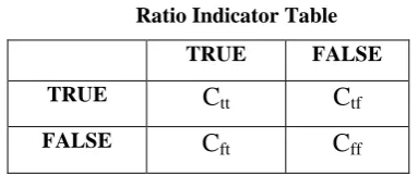
Each model’s performance is evaluated based on the accuracy derived from the confidence matrix of the
prediction output. A confusion matrix is a summary of prediction results on a classification problem, where
correct and incorrect predictions are summarized with count values and broken down by each class. Table 6
gives an overview of confusion matrix for two categories of output classes, where rows refer to class outputs in
actual test data and columns refer to class outputs from prediction.
Table 6
Ratio Indicator Table
TRUE FALSE
TRUE
C
ttC
tfFALSE
C
ftC
ffIt is obvious from Table 6 that total occurrences of correct predictions amount to
(C
tt+ C
ff)
and totaloccurrences of incorrect predictions amount to
(C
tt+ C
tf+ C
ft+ C
ff)
. Thus, accuracy for two class outputscan be derived from the formula:
a = (C
tt+ C
ff) / (C
tt+ C
tf+ C
ft+ C
ff) * 100
.4.2. Forecast Results
The forecast accuracy percentage (accurate to two decimal point digits) has been obtained from each models
confusion matrix and it refers to the percentage for which the model could accurately predict the profitability in
10-528 | P a g e
fold Cross validation approach (original data set split into multiple part for model fit) has been used to fit each
of the models in the dataset for accurate estimation. Whereas Grid Search approach has been tried to select the
hyper parameters of the different models.
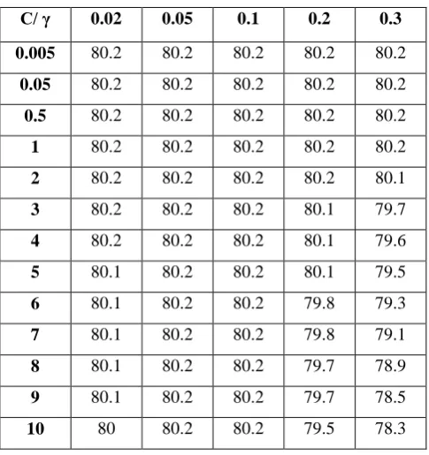
The Support Vector Machine study used different set of experiments to find out the best accuracy prediction of
SVM with respect to various kernel parameters and constants. The value of γ (kernel parameter) was
experimented within a range of 0.0001 to 1, whereas the parameter C (constant) was experimented between 0.01
and 15. Table 7 presents the best results of prediction accuracy of SVMs considering the mentioned two
parameters, where γ varies from 0.02 to 0.3 and C varies from 0.005 to 10.
Table 7
SVM Prediction Table
C/ γ 0.02 0.05 0.1 0.2 0.3
0.005 80.2 80.2 80.2 80.2 80.2
0.05 80.2 80.2 80.2 80.2 80.2
0.5 80.2 80.2 80.2 80.2 80.2
1 80.2 80.2 80.2 80.2 80.2
2 80.2 80.2 80.2 80.2 80.1
3 80.2 80.2 80.2 80.1 79.7
4 80.2 80.2 80.2 80.1 79.6
5 80.1 80.2 80.2 80.1 79.5
6 80.1 80.2 80.2 79.8 79.3
7 80.1 80.2 80.2 79.8 79.1
8 80.1 80.2 80.2 79.7 78.9
9 80.1 80.2 80.2 79.7 78.5
10 80 80.2 80.2 79.5 78.3
As observed, the best accuracy of the out-of-sample data is recorded when
C
is less than 1 irrespective of the value ofγ
. The prediction performance of the model varies withγ
and decreases whenC
increases from 1 to 15. The best accuracy that this model could provide for out of sample data is 80.2% whenC
is less than or equal to 1 irrespective ofγ
.In case of experimenting by random forest technique, the number of trees has been varied to prepare different
models. The number of trees parameter has been varied from 50 to 10000 and the corresponding result has been
displayed in Table 8.
As can be observed from the results obtained from the Random Forest models, while the accuracy decreases
below 500 trees, but it does not get changed much when number of trees has been increased above 500. In fact,
the R program to model the Random Forest classification crashed on an 8GB machine, when the number of trees
has been increased to 50000, but the accuracy till 10000 trees did not change much. The best accuracy that
529 | P a g e
Table 8Random Forest Prediction Table
Number of Trees Accuracy
50 79.6
100 79.68
200 79.76
300 80
400 79.92
500 80
600 80
700 79.84
800 79.76
900 79.92
1000 80
1100 79.68
1200 79.84
1300 80
2000 80
5000 79.92
10000 80
In case of experimenting by Xgboost technique, the number of iterations (numIt column in Table 9) and
maximum depth of a tree (maxDepth in Table 7) have been varied to prepare different models. Number of
iterations have been tried within the range of 1 to 50, whereas maximum Tree depth has been tried with values
within the range of 1 to 15. Table 7 presents the best results of prediction accuracy of Xgboost models
considering the mentioned two parameters. NA value refers to the inability to create a model with the
combination of given parameters.
As can be observed from the results obtained from the Xgboost models, the accuracy remains constant with
80.67% when number of iterations is only 1 irrespective of the maximum Tree depth, but it gradually decreases
when maximum depth is increased for any given number of iterations. The best accuracy that Xgboost could
provide is 81.31% when number of iterations is 4 and the maximum depth of tree has been set to 3.
Table 9
Xgboost Prediction Table
numIt/maxDepth 1 2 3 4 5 6 7 8 9
1 80.67 80.67 80.67 80.67 80.67 80.67 80.67 80.67 80.67
2 NA 77.86 77.14 77.22 75.62 75.06 74.5 74.1 74.82
3 NA 81.23 81.23 80.67 79.87 78.59 77.47 75.30 75.30
4 NA 81.15 81.31 81.07 80.91 80.75 80.91 79.87 78.91
530 | P a g e
6 NA NA 81.23 81.07 80.99 80.75 80.91 80.51 80.517 NA NA NA NA 80.99 80.91 80.91 80.51 80.19
8 NA NA NA NA 80.91 80.91 81.07 80.75 80.03
9 NA NA NA NA 80.91 80.67 81.23 80.99 80.11
10 NA NA NA NA 80.91 80.75 81.15 80.83 80.27
15 NA NA NA NA 81.07 80.75 80.83 80.75 80.03
20 NA NA NA NA 81.23 80.27 80.91 80.59 79.79
25 NA NA NA NA 80.99 80.43 80.91 80.67 79.55
50 NA 81.07 80.83 80.99 80.91 80.27 81.07 80.27 78.58
Overall most of the accuracies produced by Xgboost models for any combination of these two parameters is
more than highest accuracies produced by the SVM or Random Forest models even after parameter tuning.
Thus, out of all the discussed models, Xgboost outperforms SVM and Random Forest by 1.11% and 1.31 %
respectively although marginally.
The results indicate the feasibility of Xgboost in forecasting the profitability of trades in intraday financial time
series data. Thus, this experimental study could suggest for a better approach to gauge profitability intraday
equity trading than suggested in the study performed by Kim, 2003[8].
V. CONCLUSION
This experimental study used SVM, random forest and Xgboost to predict the profitability of intraday trades in
equity market. The experimental results showed that Xgboost outperformed SVM and random forest. The
reason behind the better performance of Xgboost models over the other two models is due to the reason that
Xgboost tries to fall into local minima using Gradient Boosting considering multiple trees.
Possible application of this study is to prepare a complete trading strategy considering other measures of trading.
Since, forecasting accuracy is impressing, a complete intraday trading strategy can be implemented and back
tested.
Even though the results are promising, this study has few limitations as below:
This study does not predict the actual profits, instead it predicts whether there is possibility of profit or not. This study does not consider extensive list of parameters of effective trading such as stop loss value,
maximum drawdown, profit loss ratio, winning and losing percentages etc. Since, the proposed study is not
an extensive study of a complete trading strategy, all the mentioned trading parameters should be
considered to prepare a trading strategy.
This study uses 10-fold Cross Validation approach as used commonly in practice, but any fold Cross
Validation can certainly be experimented with.
This study considers following three-time interval from the current time interval for experiments, since it
may not be the optimal parameter, other windows of time intervals require to be experimented with.
A further study can be performed by experimenting the independent variables used for modelling the
531 | P a g e
REFERENCES
[1] Leung, M. T., Daouk, H., Chen, A. S., ―Forecasting stock indices: a comparison of classification and level
estimation models‖, International Journal of Forecasting, 16, 2000, 173–190.
[2] Kamruzzaman, J., Sarker, R. A., ―ANN-Based Forecasting of Foreign Currency Exchange Rates‖, Neural Information Processing - Letters and Reviews, 3 (2), 2004.
[3] O’ Connor, M., Remus, W., & Griggs, K., Going up-going down: ―How good are people at forecasting trends and changes in trends?‖, Journal of Forecasting, 16, 1997, 165–176.
[4] Wu, Y., & Zhang, H., ―Forward premiums as unbiased predictors of future currency depreciation: A
nonparametric analysis‖, Journal of International Money and Finance 16, 1997, 609–623.
[5] Ferson W. E., Harvey C. R.., ―The risk and predictability of international equity returns‖, Review of Financial Studies, 6, 1993, 527–66.
[6] Van E, Robert J. The application of neural networks in the forecasting of share prices. Haymarket, VA, USA: Finance & Technology Publishing, 1997.
[7] Cheng W, Wanger L, Lin CH., ―Forecasting the 30-year US treasury bond with a system of neural networks‖, Journal of Computational Intelligence in Finance, 4, 1996,10–6.
[8] Kim, K. J., ―Financial time series forecasting using support vector machines‖, Neurocomputing, 55, 2003, 307 – 319.
[9] Tay, F. E. H., Cao, L., ―Application of support vector machines in financial time series forecasting‖, Omega, 29, 2001, 309–317.
[10] V.N. Vapnik, Statistical Learning Theory, Wiley, New York, 1998.
[11] Breiman, L., ―Random Forests‖, Machine Learning, 45, 2001, 5-32.
[12] Larivière, B., Poel, D. V. D., ―Predicting Customer Retention and Profitability by Using Random Forests and Regression Forests Techniques‖, Working Paper, Department of Marketing, Hoveniersberg 24, 9000 Gent, Belgium, 2004.
[13] Creamer, G. & Freund, Y. "Predicting performance and quantifying corporate governance risk for Latin
American ADRs and banks", Proceedings of the Financial Engineering and Applications Conference, Cambridge, UK, 91-101.
[14] Tianqi Chen, Carlos Guestrin, "A Scalable Tree Boosting System", 2016.
[15] Jaffe, J., Westerfield, R., ―Patterns in Japanese common stock returns: day of the week and turn of the year
effects‖, Journal of Financial and Quantitative Analysis, 20, 1985, 261–72.
[16] Takashi, K., Kazuo, A., ―Stock Market Prediction System with Modular Neural Network‖, International Joint Conference on Neural Networks, 1, 1990, 1-6.
[17] Adam, F., Lin, L. H., ―An Analysis of the Applications of Neural Networks in Finance‖, Interfaces, 31 (4), 2001, 112–122.
[18] Qin Qin, Qing-Guo Wang, Jin Li, Shuzhi Sam Ge, "Linear and Nonlinear Trading Models with Gradient
Boosted Random Forests and Application to Singapore Stock Market", Journal of Intelligent Learning Systems and Applications, 2013, 5, 1-10.
[19] Joseph O Ogutu, Hans-Peter Piepho, Torben Schulz-Streeck, "A comparison of random forests, boosting
532 | P a g e
[20] Ivana Semanjski, Sidharta Gautama, "Smart City Mobility Application—Gradient Boosting Trees forMobility Prediction and Analysis Based on Crowdsourced Data", 2015, 15, 15974-15987.
[21] Vladimir Svetnik, Ting Wang, Christopher Tong, Andy Liaw, Robert P. Sheridan, Qinghua Song,