OReilly Statistics in a Nutshell A Desktop Quick Reference Aug 2008 pdf

Other resources from O’Reilly

Related titles Baseball Hacks™ Head First Statistics

Programming Collective Intelligence

Statistics Hacks™

oreilly.com oreilly.comis more than a complete catalog of O’Reilly books.You’ll also find links to news, events, articles, weblogs, sample chapters, and code examples.

oreillynet.comis the essential portal for developers

in-terested in open and emerging technologies, including new platforms, programming languages, and operat-ing systems.

Conferences O’Reilly brings diverse innovators together to nurture the ideas that spark revolutionary industries.We spe-cialize in documenting the latest tools and systems, translating the innovator’s knowledge into useful skills for those in the trenches.Visitconferences.oreilly.com for our upcoming events.

STATISTICS

IN A NUTSHELL

Sarah Boslaugh and Paul Andrew Watters

Statistics in a Nutshell

by Sarah Boslaugh and Paul Andrew Watters Copyright © 2008 Sarah Boslaugh. All rights reserved. Printed in the United States of America.

Published by O’Reilly Media, Inc., 1005 Gravenstein Highway North, Sebastopol, CA 95472. O’Reilly books may be purchased for educational, business, or sales promotional use.Online editions are also available for most titles (safari.oreilly.com). For more information, contact our corporate/institutional sales department: (800) 998-9938 or[email protected].

Editor: Mary Treseler

Production Editor: Sumita Mukherji

Copyeditor: Colleen Gorman

Proofreader: Emily Quill

Indexer: John Bickelhaupt

Cover Designer: Karen Montgomery

Interior Designer: David Futato

Illustrator: Robert Romano

Printing History:

July 2008: First Edition.

Nutshell Handbook, the Nutshell Handbook logo, and the O’Reilly logo are registered trademarks of O’Reilly Media, Inc. TheIn a Nutshell series designations,Statistics in a

Nutshell, the image of a thornback crab, and related trade dress are trademarks of O’Reilly

Media, Inc.

Many of the designations used by manufacturers and sellers to distinguish their products are claimed as trademarks. Where those designations appear in this book, and O’Reilly Media, Inc. was aware of a trademark claim, the designations have been printed in caps or initial caps.

While every precaution has been taken in the preparation of this book, the publisher and authors assume no responsibility for errors or omissions, or for damages resulting from the use of the information contained herein.

This book uses RepKover™_{, a durable and flexible lay-flat binding.}

v Chapter 1

Table of Contents

Preface

xi

1. Basic Concepts of Measurement

1

Measurement 2

Levels of Measurement 2

True and Error Scores 7

Reliability and Validity 8

Measurement Bias 15

Exercises 18

2. Probability

21

About Formulas 22

Basic Definitions 23

Defining Probability 29

Bayes’s Theorem 32

Enough Exposition, Let’s Do Some Statistics! 34

Exercises 36

3. Data Management

41

An Approach, Not a Set of Recipes 42

The Chain of Command 43

Codebooks 43

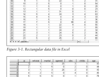
The Rectangular Data File 45

Spreadsheets and Relational Databases 47

String and Numeric Data 51

Missing Data 51

4. Descriptive Statistics and Graphics

54

Populations and Samples 54

Measures of Central Tendency 55

Measures of Dispersion 58

Outliers 62

Graphic Methods 63

Bar Charts 65

Bivariate Charts 75

Exercises 81

5. Research Design

85

Observational Studies 86

Experimental Studies 88

Gathering Experimental Data 90

Inference and Threats to Validity 96

Eliminating Bias 101

Example Experimental Design 105

6. Critiquing Statistics Presented by Others

107

The Misuse of Statistics 107

Common Problems 108

Quick Checklist 110

Research Design 111

Descriptive Statistics 113

Inferential Statistics 118

7. Inferential Statistics

125

Probability Distributions 126

Independent and Dependent Variables 132

Populations and Samples 133

The Central Limit Theorem 137

Hypothesis Testing 140

Confidence Intervals 144

p-values 145

Data Transformations 146

Exercises 149

8. The t-Test

151

Table of Contents | vii

t-Tests 152

One-Sample t-Test 155

Two-Sample t-Test 157

Repeated Measures t-Test 160

Unequal Variance t-Test 162

Effect Size and Power 164

Exercises 165

9. The Correlation Coefficient

169

Measuring Association 169

Graphing Associations Through Scatterplots 170

Pearson’s Product-Moment Correlation Coefficient 176

Coefficient of Determination 180

Spearman Rank-Order Coefficient 183

Advanced Techniques 185

10. Categorical Data

188

The R×C Table 189

The Chi-Square Distribution 190

The Chi-Square Test 191

Fisher’s Exact Test 196

McNemar’s Test for Matched Pairs 197

Correlation Statistics for Categorical Data 199

The Likert and Semantic Differential Scales 202

Exercises 203

11. Nonparametric Statistics

207

Nonnormal Data 208

Between Subjects Designs 209

Within-Subjects Designs 217

Exercises 221

12. Introduction to the General Linear Model

224

The General Linear Model 225

Linear Regression 226

Analysis of Variance (ANOVA) 232

Exercises 239

13. Extensions of Analysis of Variance

243

Factorial ANOVA 244

ANCOVA 253

Repeated Measures ANOVA 255

Mixed Designs 257

14. Multiple Linear Regression

264

Multiple Regression Models 264

Common Problems with Multiple Regression 277

Exercises 279

15. Other Types of Regression

284

Logistic Regression 284

Logarithmic Transformations 287

Polynomial Regression 288

Overfitting 292

16. Other Statistical Techniques

298

Factor Analysis 298

Cluster Analysis 305

Discriminant Function Analysis 309

Multidimensional Scaling 312

17. Business and Quality Improvement Statistics

315

Index Numbers 315

Time Series 319

Decision Analysis 323

Quality Improvement 328

Exercises 335

18. Medical and Epidemiological Statistics

339

Measures of Disease Frequency 339

Ratio, Proportion, and Rate 340

Prevalence and Incidence 342

Crude, Category-Specific, and Standardized Rates 345

The Risk Ratio 348

The Odds Ratio 352

Confounding, Stratified Analysis, and the

Mantel-Haenszel Common Odds Ratio 354

Power Analysis 358

Sample Size Calculations 361

Table of Contents | ix

19. Educational and Psychological Statistics

366

Percentiles 367 Standardized Scores 369 Test Construction 370 Classical Test Theory: The True Score Model 373 Reliability of a Composite Test 374 Measures of Internal Consistency 375 Item Analysis 379 Item Response Theory 383 Exercises 388

A. Review of Basic Mathematics

391

B. Introduction to Statistical Packages

414

C. References

431

xi Chapter 2

Preface

One thing I (Sarah) have learned over the last 20 or so years is that a sure way to derail a promising conversation at a party is to tell people what I do for a living. And rest assured that I’m neither a tax auditor nor captain of a sludge barge.No, I’m merely a biostatistician and statistics instructor, a revelation which invariably provokes a response such as “statistics was my worst class in school” or the sudden inspiration to quote that old chestnut popularized by Mark Twain that there are three kinds of lies: lies, damned lies, and statistics.

Personally, I find statistics fascinating and I love working in this field.I like teaching statistics as well, and I like to believe that I communicate some of this enthusiasm to my students, most of whom are physicians or other healthcare professionals required to take my classes as part of their fellowship studies.It’s often an uphill battle, however: some of them arrive with a negative attitude toward everything statistical, possibly augmented by the belief that statistics is some kind of magical procedure that will do their thinking for them, or a set of tricks and manipulations whose purpose is to twist reality in order to mislead other people.

What Is Statistics?

Before we jump into the technical details of learning and using statistics, let’s step back for a minute and consider what can be meant by the word “statistics.” Don’t worry if you don’t understand all the vocabulary immediately: it will become clear over the course of this book.

When people speak of statistics, they usually mean one or more of the following: 1. Numerical data such as the unemployment rate, the number of persons who

die annually from bee stings, or the racial makeup of the population of New York City in 2006 as compared to 1906.

2. Numbers used to describe samples (subsets) of data, such as the mean (average), as opposed to numbers used to describe populations (entire sets of data); for instance, if we work for an advertising firm interested in the average age of people who subscribe toSports Illustrated, we can draw a sample of subscribers and calculate the mean of that sample (a statistic), which is an estimate of the mean of the entire population of subscribers.

3. Particular procedures used to analyze data, and the results of those proce-dures, such as thet statistic or the chi-square statistic.

4. A field of study that develops and uses mathematical procedures to describe data and make decisions regarding it.

The type of statistics referred to in definition #1 is not the primary concern of this book: if you simply want to find the latest figures on unemployment, health, or any of the myriad other topics on which governments and private organizations regularly release statistical data, your best bet is to consult a reference librarian or subject expert.If, however, you want to know how to interpret those figures (to understand why the mean is often misleading as a statement of average value, for instance, or the difference between crude and standardized mortality rates),

Statis-tics in a Nutshell can definitely help you out.

The concepts included in definition #2 will be discussed in Chapter 7, which introduces inferential statistics, but they also permeate this book.It is partly a question of vocabulary (statisticsare numbers that describesamples, while

param-etersare numbers that describepopulations), but also underscores a fundamental

point about the practice of statistics.The concept of using information gained from studying a sample to make statements about a population is the basis of inferential statistics, and inferential statistics is the primary focus of this book (as it is of most books about statistics).

Preface | xiii to understand and interpret statistics has far outstripped the need to learn how to do the calculations themselves.

Definition #4 is nearest to my heart, since I chose statistics as my professional field.If you are a secondary or post-secondary student you are probably aware of this definition of statistics, as many universities and colleges today either have a separate department of statistics or include statistics as a field of specialization within mathematics.Statistics is increasingly taught in high school as well: in the U.S., enrollment in the A.P. (Advanced Placement) Statistics classes is increasing more rapidly than enrollment in any other A.P. area.

Statistics is too important to be left to the statisticians, however, and university study in many subjects requires one or more semesters of statistics classes.Many basic techniques in modern statistics have been developed by people who learned and used statistics as part of their studies in another field.For instance, Stephen Raudenbush, a pioneer in the development of hierarchical linear modeling, studied Policy Analysis and Evaluation Research at Harvard, and Edward Tufte, perhaps the world’s leading expert on statistical graphics, began his career as a political scientist: his Ph.D. dissertation at Yale was on the American Civil Rights Movement.

With the increasing use of statistics in many professions, and at all levels from top to bottom, basic knowledge of statistics has become a necessity for many people who have been out of school for years.Such individuals are often ill-served by textbooks aimed at introductory college courses, which are too specialized, too focused on calculation, and too expensive.

Finally, statistics cannot be left to the statisticians because it’s also a necessity to understand much of what you read in the newspaper or hear on television and the radio.A working knowledge of statistics is the best check against the proliferation of misleading or outright false claims (whether by politicians, advertisers, or social reformers), which seem to occupy an ever-increasing portion of our daily news diet.There’s a reason that Darryl Huff’s 1954 classic How to Lie with Statistics (W.W. Norton) remains in print: statistics are easy to misuse, the common tech-niques of statistical distortion have been around for decades, and the best defense against those who would lie with statistics is to educate yourself so you can spot the lies and stop the lying liars in their tracks.

The Focus of This Book

There are so many statistics books already on the market that you might well wonder why we feel the need to add another to the pile.The primary reason is that we haven’t found any statistics books that answer the needs we have addressed inStatistics in a Nutshell.In fact, if I may wax poetic for a moment, the situation is, to paraphrase the plight of Coleridge’s Ancient Mariner, “books, books everywhere, nor any with which to learn.” The issues we have tried to address with this book are:

2. The need to integrate discussion of issues such as measurement and data management into an introductory statistics text.

3. The need for a book that isn’t focused on a particular subject area.Elemen-tary statistics is largely the same across subjects (at-test is pretty much the same whether the data comes from medicine, finance, or criminal justice), so there’s no need for a proliferation of texts presenting the same information with slightly different spin.

4. The need for an introductory statistics book that is compact, inexpensive, and easy for beginners to understand without being condescending or overly simplistic.

So who is the intended audience of Statistics in a Nutshell? We see three in particular:

1. Students taking introductory statistics classes in high schools, colleges, and universities.

2. Adults who need to learn statistics as part of their current jobs or in order to be eligible for promotion.

3. People who are interested in learning about statistics out of intellectual curiosity.

Our focus throughout Statistics in a Nutshell is not on particular techniques, although many are taught within this work, but on statistical reasoning.You might say that our focus is not on doing statistics, but on thinking statistically. What does that mean? Several things are necessary in order to be able to focus on the process of thinking with numbers.More particularly, we focus on thinking about data, and using statistics to aid in that process.

Statistics in the Age of Information

It’s become fashionable to say that we’re living in the Age of Information, where so many facts are collected and disseminated that no one could possibly keep up with them.Well, this is one of those clichés that is based on truth: we are drowning in data and the problem is only going to get worse.Wide access to computing technology and electronic means of data storage and dissemination have made information easier to access, which is great from the researcher’s point of view, since you no longer have to travel to a particular library or archive to peruse printed copies of records.

Preface | xv

Organization of This Book

Statistics in a Nutshellis organized into four parts: introductory material

(Chap-ters 1–6) that lays the necessary foundation for the chapters that follow; elementary inferential statistical techniques (Chapters 7–11); more advanced tech-niques (Chapters 12-16); and specialized techtech-niques (Chapters 17–19).

Here’s a more detailed breakdown of the chapters: Chapter 1,Basic Concepts of Measurement

Discusses foundational issues for statistics, including levels of measurement, operationalization, proxy measurement, random and systematic error, measures of agreement, and types of bias.Statistics demonstrated include percent agreement and kappa.

Chapter 2,Probability

Introduces the basic vocabulary and laws of probability, including trials, events, independence, mutual exclusivity, the addition and multiplication laws, and conditional probability.Procedures demonstrated include calcula-tion of basic probabilities, permutacalcula-tions and combinacalcula-tions, and Bayes’s theorem.

Chapter 3,Data Management

Discusses practical issues in data management, including procedures to troubleshoot an existing file, methods for storing data electronically, data types, and missing data.

Chapter 4,Descriptive Statistics and Graphics

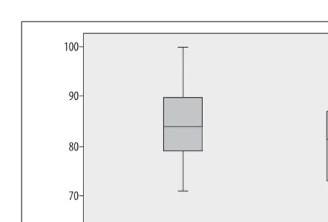
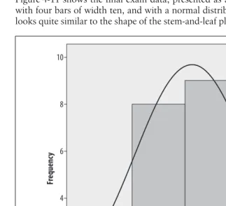
Explains the differences between descriptive and inferential statistics and between populations and samples, and introduces common measures of central tendency and variability and frequently used graphs and charts.Statis-tics demonstrated include mean, median, mode, range, interquartile range, variance, and standard deviation.Graphical methods demonstrated include frequency tables, bar charts, pie charts, Pareto charts, stem and leaf plots, boxplots, histograms, scatterplots, and line graphs.

Chapter 5,Research Design

Discusses observational and experimental studies, common elements of good research designs, the steps involved in data collection, types of validity, and methods to limit or eliminate the influence of bias.

Chapter 6,Critiquing Statistics Presented by Others

Offers guidelines for reviewing the use of statistics, including a checklist of questions to ask of any statistical presentation and examples of when legiti-mate statistical procedures may be manipulated to appear to support questionable conclusions.

Chapter 7,Inferential Statistics

converting raw scores to Z-scores, calculation of binomial probabilities, and the square-root and log data transformations.

Chapter 8,The t-Test

Discusses thet-distribution, the different types oft-tests, and the influence of effect size on power int-tests.Statistics demonstrated include the one-sample t-test, the two independent samples t-test, the two repeated measurest-test, and the unequal variancet-test.

Chapter 9,The Correlation Coefficient

Introduces the concept of association with graphics displaying different strengths of association between two variables, and discusses common statis-tics used to measure association.Statisstatis-tics demonstrated include Pearson’s product-moment correlation, thet-test for statistical significance of Pearson’s correlation, the coefficient of determination, Spearman’s rank-order coeffi-cient, the point-biserial coefficoeffi-cient, and phi.

Chapter 10,Categorical Data

Reviews the concepts of categorical and interval data, including the Likert scale, and introduces the R×C table.Statistics demonstrated include the chi-squared tests for independence, equality of proportions, and goodness of fit, Fisher’s exact test, McNemar’s test, gamma, Kendall’s tau-a, tau-b, and tau-c, and Somers’s d.

Chapter 11,Nonparametric Statistics

Discusses when to use nonparametric rather than parametric statistics, and presents nonparametric statistics for between-subjects and within-subjects designs.Statistics demonstrated include the Wilcoxon Rank Sum and Mann-Whitney U tests, the median test, the Kruskal-Wallis H test, the Wilcoxon matched pairs signed rank test, and the Friedman test.

Chapter 12,Introduction to the General Linear Model

Introduces linear regression and ANOVA through the concept of the General Linear Model, and discusses assumptions made when using these designs. Statistical procedures demonstrated include simple (bivariate) regression, one-way ANOVA, and post-hoc testing.

Chapter 13,Extensions of Analysis of Variance

Discusses more complex ANOVA designs.Statistical procedures demon-strated include two-way and three-way ANOVA, MANOVA, ANCOVA, repeated measures ANOVA, and mixed designs.

Chapter 14,Multiple Linear Regression

Extends the ideas introduced in Chapter 12 to models with multiple predic-tors.Topics covered include relationships among predictor variables, standardized coefficients, dummy variables, methods of model building, and violations of assumptions of linear regression, including nonlinearity, auto-correlation, and heteroscedasticity.

Chapter 15,Other Types of Regression

Preface | xvii Chapter 16,Other Statistical Techniques

Demonstrates several advanced statistical procedures, including factor anal-ysis, cluster analanal-ysis, discriminant function analanal-ysis, and multidimensional scaling, including discussion of the types of problems for which each tech-nique may be useful.

Chapter 17,Business and Quality Improvement Statistics

Demonstrates statistical procedures commonly used in business and quality improvement contexts.Analytical and statistical procedures covered include construction and use of simple and composite indexes, time series, the minimax, maximax, and maximin decision criteria, decision making under risk, decision trees, and control charts.

Chapter 18,Medical and Epidemiological Statistics

Introduces concepts and demonstrates statistical procedures particularly rele-vant to medicine and epidemiology.Concepts and statistics covered include the definition and use of ratios, proportions, and rates, measures of preva-lence and incidence, crude and standardized rates, direct and indirect standardization, measures of risk, confounding, the simple and Mantel-Haenszel odds ratio, and precision, power, and sample size calculations. Chapter 19,Educational and Psychological Statistics

Introduces concepts and statistical procedures commonly used in the fields of education and psychology.Concepts and procedures demonstrated include percentiles, standardized scores, methods of test construction, the true score model of classical test theory, reliability of a composite test, measures of internal consistency including coefficient alpha, and procedures for item anal-ysis. An overview of item response theory is also provided

Two appendixes cover topics that are a necessary background to the material covered in the main text, and a third provides references to supplemental reading: Appendix A

Provides a self-test and review of basic arithmetic and algebra for people whose memory of their last math course is fast receding on the distant horizon.Topics covered include the laws of arithmetic, exponents, roots and logs, methods to solve equations and systems of equations, fractions, facto-rials, permutations, and combinations.

Appendix B

Provides an introduction to some of the most common computer programs used for statistical applications, demonstrates basic analyses in each program, and discusses their relative strengths and weaknesses.Programs covered include Minitab, SPSS, SAS, and R; the use of Microsoft Excel (not a statis-tical package) for statisstatis-tical analysis is also discussed.

Appendix C

You should think of these chapters as tools, whose best use depends on the indi-vidual reader’s, background and needs.Even the introductory chapters may not be relevant immediately to everyone: for instance, many introductory statistics classes do not require students to master topics such as data management or measurement theory.In that case, these chapters can serve as references when the topics become necessary (expertise in data management is often an expectation of research assistants, for instance, although it is rarely directly taught).

Classification of what is “elementary” and what is “advanced” depends on an individual’s background and purposes.We designed Statistics in a Nutshell to answer the needs of many different types of users.For this reason, there’s no perfect way to organize the material to meet everyone’s needs, which brings us to an important point: there’s no reason you should feel the need to read the chap-ters in the order they are presented here.Statistics presents many chicken-and-egg dilemmas: for instance, you can’t design experiments without knowing what statistics are available to you, but you can’t understand how statistics are used without knowing something about research design.Similarly, it might seem that a chapter on data management would be most useful to individuals who have already done some statistical analysis, but I’ve advised many research assistants and project managers who are put in charge of large data sets before they’ve had a single course in statistics.So use the chapters in the way that best facilitates your specific purposes, and don’t be shy about skipping around and focusing on what-ever meets your particular needs.

Some of the later chapters are also specialized and not relevant to everyone, most obviously Chapters 17–19, which are written with particular subject areas in mind.Chapters 15 and 16 also cover topics that are not often included in intro-ductory statistics texts, but that are the statistical procedure of choice in particular contexts.Because we have planned this book to be useful for consumers of statis-tics and working professionals who deal with statisstatis-tics even if they don’t compute them themselves, we have included these topics, although beginning students may not feel the need to tackle them in their first statistics course.

It’s wise to keep an open mind regarding what statistics you need to know.You may currently believe that you will never have the need to conduct a nonpara-metric test or a logistic regression analysis.However, you never know what will come in handy in the future.It’s also a mistake to compartmentalize too much by subject field: because statistical techniques are ultimately about numbers rather than content, techniques developed in one field often prove to be useful in another.For instance, control charts (covered in Chapter 17) were developed in a manufacturing context, but are now used in many fields from medicine to education.

Preface | xix

Symbols Used in This Book

Conventions Used in This Book

The following typographical conventions are used in this book: Plain text

Indicates menu titles, menu options, menu buttons, and keyboard accelera-tors (such as Alt and Ctrl).

Symbol Meaning

Names of statistics

µ Mean of a population

σ Standard deviation of a population

σ2 _{Variance of a population} Π Proportion of a population

x Mean of a sample

s Standard deviation of a sample

s2 _{Variance of a sample}

n Number of cases in a sample

p Proportion of a sample

Κ Kappa (measure of agreement)

χ2 _{Chi-squared (statistic, distribution)} Statistical formulas

Σ Summation

! Factorial

C Combination

P Permutation

E Expected value

O Observed value

x_ij Value of variable x for case ij

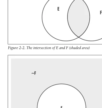
Set theory, Bayes Theorem

~ Not

| Conditional probability

∪ Union

∩ Intersection

Other

α Alpha (significance level; probability of Type I error)

Italic

Indicates new terms, URLs, email addresses, filenames, file extensions, path-names, directories, and Unix utilities

Constant width

Indicates examples

This icon signifies a tip, suggestion, or general note.

We’d Like to Hear From You

Please address comments and questions concerning this book to the publisher: O’Reilly Media, Inc.

1005 Gravenstein Highway North Sebastopol, CA 95472

800-998-9938 (in the United States or Canada) 707-829-0515 (international or local)

707-829-0104 (fax)

We have a web page for this book, where we list errata, examples, and any addi-tional information. You can access this page at:

http://www.oreilly.com/catalog/9780596510497

To comment or ask technical questions about this book, send email to: [email protected]

For more information about our books, conferences, Resource Centers, and the O’Reilly Network, see our website at:

http://www.oreilly.com

Safari® Books Online

When you see a Safari® Books Online icon on the cover of your favorite technology book, that means the book is available online through the O’Reilly Network Safari Bookshelf.

Preface | xxi

Acknowledgments

Only two authors are listed on the cover of this book, but the contributions of many people played a role in its creation.

Sarah Boslaugh

I would like to thank my agent, Neil Salkind, for his continued guidance and support; my colleagues at Washington University and BJC HealthCare for their willingness to share their wisdom and experience; the crew at O’Reilly, including Mary Treseler, Isabel Kunkle, Rachel Monaghan, and Colleen Gorman; and the statisticians who assisted in the technical review process, especially Dave McArthur at UCLA who is never shy about sharing his suggestions.I would also like to thank all my friends who keep pestering me to explain statistical concepts to them, and thus encouraged me to write this book.On a personal note, I would like to thank my colleague Rand Ross at Washington University for helping me remain sane throughout the writing process, and my husband Dan Peck for being the very model of a modern supportive spouse.

Paul Watters

1 Chapter 1Basic Concepts

1

Basic Concepts of Measurement

Before you can use statistics to analyze a problem, you must convert the basic materials of the problem to data.That is, you must establish or adopt a system of assigning values, most often numbers, to the objects or concepts that are central to the problem under study.This is not an esoteric process, but something you do every day.For instance, when you buy something at the store, the price you pay is a measurement: it assigns a number to the amount of currency that you have exchanged for the goods received.Similarly, when you step on the bathroom scale in the morning, the number you see is a measurement of your body weight. Depending on where you live, this number may be expressed in either pounds or kilograms, but the principle of assigning a number to a physical quantity (weight) holds true in either case.

Not all data need be numeric.For instance, the categoriesmale andfemale are commonly used in both science and in everyday life to classify people, and there is nothing inherently numeric in these categories.Similarly, we often speak of the colors of objects in broad classes such as “red” or “blue”: these categories of which represent a great simplification from the infinite variety of colors that exist in the world.This is such a common practice that we hardly give it a second thought.

Measurement

Measurement is the process of systematically assigning numbers to objects and

their properties, to facilitate the use of mathematics in studying and describing objects and their relationships.Some types of measurement are fairly concrete: for instance, measuring a person’s weight in pounds or kilograms, or their height in feet and inches or in meters.Note that the particular system of measurement used is not as important as a consistent set of rules: we can easily convert measure-ment in kilograms to pounds, for instance.Although any system of units may seem arbitrary (try defending feet and inches to someone who grew up with the metric system!), as long as the system has a consistent relationship with the prop-erty being measured, we can use the results in calculations.

Measurement is not limited to physical qualities like height and weight.Tests to measure abstractions like intelligence and scholastic aptitude are commonly used in education and psychology, for instance: the field of psychometrics is largely concerned with the development and refinement of methods to test just such abstract qualities.Establishing that a particular measurement is meaningful is more difficult when it can’t be observed directly: while you can test the accuracy of a scale by comparing the results with those obtained from another scale known to be accurate, there is no simple way to know if a test of intelligence is accurate because there is no commonly agreed-upon way to measure the abstraction “intel-ligence.” To put it another way, we don’t know what someone’s actual intelligence is because there is no certain way to measure it, and in fact we may not even be sure what “intelligence” really is, a situation quite different from that of measuring a person’s height or weight.These issues are particularly relevant to the social sciences and education, where a great deal of research focuses on just such abstract concepts.

Levels of Measurement

Statisticians commonly distinguish four types or levels of measurement; the same terms may also be used to refer to data measured at each level.The levels of measurement differ both in terms of the meaning of the numbers and in the types of statistics that are appropriate for their analysis.

Nominal Data

Withnominaldata, as the name implies, the numbers function as anameor label

Levels of Measurement | 3

Basic Concepts

years of experience and salary in baseball players, you might classify the players according to their primary position by using the traditional system whereby 1 is assigned to pitchers, 2 to catchers, 3 to first basemen, and so on.

If you can’t decide whether data is nominal or some other level of measurement, ask yourself this question: do the numbers assigned to this data represent some quality such that a higher value indicates that the object has more of that quality than a lower value? For instance, is there some quality “gender” which men have more of than women? Clearly not, and the coding scheme would work as well if women were coded as 1 and men as 0.The same principle applies in the baseball example: there is no quality of “baseballness” of which outfielders have more than pitchers.The numbers are merely a convenient way to label subjects in the study, and the most important point is that every position is assigned a distinct value. Another name for nominal data iscategoricaldata, referring to the fact that the measurements place objects into categories (male or female; catcher or first baseman) rather than measuring some intrinsic quality in them.Chapter 10 discusses methods of analysis appropriate for this type of data, and many tech-niques covered in Chapter 11, on nonparametric statistics, are also appropriate for categorical data.

When data can take on only two values, as in the male/female example, it may also be calledbinarydata.This type of data is so common that special techniques have been developed to study it, including logistic regression (discussed in Chapter 15), which has applications in many fields.Many medical statistics such as the odds ratio and the risk ratio (discussed in Chapter 18) were developed to describe the relationship between two binary variables, because binary variables occur so frequently in medical research.

Ordinal Data

Ordinaldata refers to data that has some meaningfulorder, so that higher values

represent more of some characteristic than lower values.For instance, in medical practice burns are commonly described by their degree, which describes the amount of tissue damage caused by the burn.A first-degree burn is characterized by redness of the skin, minor pain, and damage to the epidermis only, while a second-degree burn includes blistering and involves the dermis, and a third-degree burn is characterized by charring of the skin and possibly destroyed nerve endings.These categories may be ranked in a logical order: first-degree burns are the least serious in terms of tissue damage, third-degree burns the most serious. However, there is no metric analogous to a ruler or scale to quantify how great the distance between categories is, nor is it possible to determine if the difference between first- and second-degree burns is the same as the difference between second- and third-degree burns.

while not assuming any further properties of the scales.For instance, it is appro-priate to calculate the median (central value) of ordinal data, but not the mean (which assumes interval data).Some of these techniques are discussed later in this chapter, and others are covered in Chapter 11.

Interval Data

Intervaldata has a meaningful order and also has the quality that equal intervals

between measurements represent equal changes in the quantity of whatever is being measured.The most common example of interval data is the Fahrenheit temperature scale.If we describe temperature using the Fahrenheit scale, the difference between 10 degrees and 25 degrees (a difference of 15 degrees) repre-sents the same amount of temperature change as the difference between 60 and 75 degrees.Addition and subtraction are appropriate with interval scales: a differ-ence of 10 degrees represents the same amount over the entire scale of temperature.However, the Fahrenheit scale, like all interval scales, has no natural zero point, because 0 on the Fahrenheit scale does not represent an absence of temperature but simply a location relative to other temperatures.Multiplication and division are not appropriate with interval data: there is no mathematical sense in the statement that 80 degrees is twice as hot as 40 degrees.Interval scales are a rarity: in fact it’s difficult to think of another common example.For this reason, the term “interval data” is sometimes used to describe both interval and ratio data (discussed in the next section).

Ratio Data

Ratiodata has all the qualities of interval data (natural order, equal intervals) plus

a natural zero point.Many physical measurements are ratio data: for instance, height, weight, and age all qualify.So does income: you can certainly earn 0 dollars in a year, or have 0 dollars in your bank account.With ratio-level data, it is appropriate to multiply and divide as well as add and subtract: it makes sense to say that someone with $100 has twice as much money as someone with $50, or that a person who is 30 years old is 3 times as old as someone who is 10 years old. It should be noted that very few psychological measurements (IQ, aptitude, etc.) are truly interval, and many are in fact ordinal (e.g., value placed on education, as indicated by a Likert scale).Nonetheless, you will sometimes see interval or ratio techniques applied to such data (for instance, the calculation of means, which involves division).While incorrect from a statistical point of view, sometimes you have to go with the conventions of your field, or at least be aware of them.To put it another way, part of learning statistics is learning what is commonly accepted in your chosen field of endeavor, which may be a separate issue from what is accept-able from a purely mathematical standpoint.

Continuous and Discrete Data

Levels of Measurement | 5

Basic Concepts

In the course of data analysis and model building, researchers sometimes recode continuous data in categories or larger units.For instance, weight may be recorded in pounds but analyzed in 10-pound increments, or age recorded in years but analyzed in terms of the categories0–17,18–65, andover 65.From a statistical point of view, there is no absolute point when data become continuous or discrete for the purposes of using particular analytic techniques: if we record age in years, we are still imposing discrete categories on a continuous variable. Various rules of thumb have been proposed: for instance, some researchers say that when a variable has 10 or more categories (or alternately, 16 or more catego-ries), it can safely be analyzed as continuous.This is another decision to be made on a case-by-case basis, informed by the usual standards and practices of your particular discipline and the type of analysis proposed.

Discrete data can only take on particular values, and has clear boundaries.As the old joke goes, you can have 2 children or 3 children, but not 2.37 children, so “number of children” is a discrete variable.In fact, any variable based on counting is discrete, whether you are counting the number of books purchased in a year or the number of prenatal care visits made during a pregnancy.Nominal data is also discrete, as are binary and rank-ordered data.

Operationalization

Beginners to a field often think that the difficulties of research rest primarily in statistical analysis, and focus their efforts on learning mathematical formulas and computer programming techniques in order to carry out statistical calculations. However, one major problem in research has very little to do with either mathe-matics or statistics, and everything to do with knowing your field of study and thinking carefully through practical problems.This is the problem of

operational-ization, which means the process of specifying how a concept will be defined and

measured.Operationalization is a particular concern in the social sciences and education, but applies to other fields as well.

Operationalization is always necessary when a quality of interest cannot be measured directly.An obvious example is intelligence: there is no way to measure intelligence directly, so in the place of such a direct measurement we accept some-thing that we can measure, such as the score on an IQ test.Similarly, there is no direct way to measure “disaster preparedness” for a city, but we can operation-alize the concept by creating a checklist of tasks that should be performed and giving each city a “disaster preparedness” score based on the number of tasks completed and the quality or thoroughness of completion.For a third example, we may wish to measure the amount of physical activity performed by subjects in a study: if we do not have the capacity to directly monitor their exercise behavior, we may operationalize “amount of physical activity” as the amount indicated on a self-reported questionnaire or recorded in a diary.

diseases.“Burden of disease” and “suffering,” on the other hand, are concepts that could be used to define appropriate outcomes for many studies, but that have no direct means of measurement and must therefore be operationalized.Exam-ples of operationalization of burden of disease include measurement of viral levels in the bloodstream for patients with AIDS and measurement of tumor size for people with cancer.Decreased levels of suffering or improved quality of life may be operationalized as higher self-reported health state, higher score on a survey instrument designed to measure quality of life, improved mood state as measured through a personal interview, or reduction in the amount of morphine requested. Some argue that measurement of even physical quantities such as length require operationalization, because there are different ways to measure length (a ruler might be the appropriate instrument in some circumstances, a micrometer in others). However, the problem of operationalization is much greater in the human sciences, when the object or qualities of interest often cannot be measured directly.

Proxy Measurement

The term proxy measurementrefers to the process of substituting one measure-ment for another.Although deciding on proxy measuremeasure-ments can be considered as a subclass of operationalization, we will consider it as a separate topic.The most common use of proxy measurement is that of substituting a measurement that is inexpensive and easily obtainable for a different measurement that would be more difficult or costly, if not impossible, to collect.

For a simple example of proxy measurement, consider some of the methods used by police officers to evaluate the sobriety of individuals while in the field.Lacking a portable medical lab, an officer can’t directly measure blood alcohol content to determine if a subject is legally drunk or not.So the officer relies on observation of signs associated with drunkenness, as well as some simple field tests that are believed to correlate well with blood alcohol content.Signs of alcohol intoxica-tion include breath smelling of alcohol, slurred speech, and flushed skin.Field tests used to quickly evaluate alcohol intoxication generally require the subjects to perform tasks such as standing on one leg or tracking a moving object with their eyes.Neither the observed signs nor the performance measures are direct measures of inebriation, but they are quick and easy to administer in the field. Individuals suspected of drunkenness as evaluated by these proxy measures may then be subjected to more accurate testing of their blood alcohol content.

True and Error Scores | 7

Basic Concepts

Proxy measurements are most useful if, in addition to being relatively easy to obtain, they are good indicators of the true focus of interest.For instance, if correct execution of prescribed processes of medical care for a particular treat-ment is closely related to good patient outcomes for that condition, and if poor or nonexistent execution of those processes is closely related to poor patient outcomes, then execution of these processes is a useful proxy for quality.If that close relationship does not exist, then the usefulness of measurements of those processes as a proxy for quality of care is less certain.There is no mathematical test that will tell you whether one measure is a good proxy for another, although computing statistics like correlations or chi-squares between the measures may help evaluate this issue.Like many measurement issues, choosing good proxy measurements is a matter of judgment informed by knowledge of the subject area, usual practices in the field, and common sense.

True and Error Scores

We can safely assume that no measurement is completely accurate.Because the process of measurement involves assigning discrete numbers to a continuous world, even measurements conducted by the best-trained staff using the finest available scientific instruments are not completely without error.One concern of measurement theory is conceptualizing and quantifying the degree of error present in a particular set of measurements, and evaluating the sources and conse-quences of that error.

Classical measurement theory conceives of any measurement or observed score as consisting of two parts: true score, and error.This is expressed in the following formula:

X = T + E

where X is the observed measurement, T is the true score, and E is the error.For instance, the bathroom scale might measure someone’s weight as 120 pounds, when that person’s true weight was 118 pounds and the error of 2 pounds was due to the inaccuracy of the scale. This would be expressed mathematically as:

120 = 118 + 2

Random and Systematic Error

Because we live in the real world rather than a Platonic universe, we assume that all measurements contain some error.But not all error is created equal.Random

erroris due to chance: it takes no particular pattern and is assumed to cancel itself

out over repeated measurements.For instance, the error scores over a number of measurements of the same object are assumed to have a mean of zero.So if someone is weighed 10 times in succession on the same scale, we may observe slight differences in the number returned to us: some will be higher than the true value, and some will be lower.Assuming the true weight is 120 pounds, perhaps the first measurement will return an observed weight of 119 pounds (including an error of –1 pound), the second an observed weight of 122 pounds (for an error of +2 pounds), the third an observed weight of 118.5 pounds (an error of –1.5 pounds) and so on.If the scale is accurate and the only error is random, the average error over many trials will be zero, and the average observed weight will be 120 pounds.We can strive to reduce the amount of random error by using more accurate instruments, training our technicians to use them correctly, and so on, but we cannot expect to eliminate random error entirely.

Two other conditions are assumed to apply to random error: it must be unrelated to the true score, and the correlation between errors is assumed to be zero.The first condition means that the value of the error component is not related to the value of the true score.If we measured the weights of a number of different indi-viduals whose true weights differed, we would not expect the error component to have any relationship to their true weights.For instance, the error component should not systematically be larger when the true weight is larger.The second condition means that the error for each score is independent and unrelated to the error for any other score: for instance, there should not be a pattern of the size of error increasing over time (which might indicate that the scale was drifting out of calibration).

In contrast,systematic errorhas an observable pattern, is not due to chance, and often has a cause or causes that can be identified and remedied.For instance, the scale might be incorrectly calibrated to show a result that is five pounds over the true weight, so the average of the above measurements would be 125 pounds, not 120.Systematic error can also be due to human factors: perhaps we are reading the scale’s display at an angle so that we see the needle as registering five pounds higher than it is truly indicating.A scale drifting higher (so the error components are random at the beginning of the experiment, but later on are consistently high) is another example of systematic error.A great deal of effort has been expended to identify sources of systematic error and devise methods to identify and eliminate them: this is discussed further in the upcoming section on measurement bias.

Reliability and Validity

There are many ways to assign numbers or categories to data, and not all are equally useful.Two standards we use to evaluate measurements arereliabilityand

validity.Ideally, every measure we use should be both reliable and valid.In reality,

Reliability and Validity | 9

Basic Concepts

circumstance: a measure that is highly reliable when used with one group of people may be unreliable when used with a different group, for instance.For this reason it is more useful to evaluate how valid and reliable a measure is for a particular purpose and whether the levels of reliability and validity are acceptable in the context at hand.Reliability and validity are also discussed in Chapter 5, in the context of research design, and in Chapter 19, in the context of educational and psychological testing.

Reliability

Reliability refers to how consistent or repeatable measurements are.For instance, if we give the same person the same test on two different occasions, will the scores be similar on both occasions? If we train three people to use a rating scale designed to measure the quality of social interaction among individuals, then showed each of them the same film of a group of people interacting and asked them to evaluate the social interaction exhibited in the film, will their ratings be similar? If we have a technician measure the same part 10 times, using the same instrument, will the measurements be similar each time? In each case, if the answer is yes, we can say the test, scale, or instrument is reliable.

Much of the theory and practice of reliability was developed in the field of educa-tional psychology, and for this reason, measures of reliability are often described in terms of evaluating the reliability of tests.But considerations of reliability are not limited to educational testing: the same concepts apply to many other types of measurements including opinion polling, satisfaction surveys, and behavioral ratings.

The discussion in this chapter will be kept at a fairly basic level: information about calculating specific measures of reliability are discussed in more detail in Chapter 19, in connection with test theory.In addition, many of the measures of reliability draw on thecorrelation coefficient(also called simply thecorrelation), which is discussed in detail in Chapter 9, so beginning statisticians may want to concentrate on the logic of reliability and validity and leave the details of evalu-ating them until after they have mastered the concept of the correlation coefficient.

There are three primary approaches to measuring reliability, each useful in partic-ular contexts and each having particpartic-ular advantages and disadvantages:

• Multiple-occasions reliability • Multiple-forms reliability • Internal consistency reliability

Multiple-occasions reliability,sometimes calledtest-retest reliability, refers to how

a patient whose state may have changed over the two-week period.Multiple-occasions reliability is not a suitable measure for volatile qualities, such as mood state.It is also unsuitable if the focus of measurement may have changed over the time period between tests (for instance, if the student learned more about a subject between the testing periods) or may be changed as a result of the first testing (for instance, if a student remembers what questions were asked on the first test administration).A common technique for assessing multiple-occasions reliability is to compute the correlation coefficient between the scores from each occasion of testing: this is called thecoefficient of stability.

Multiple-forms reliability(also calledparallel-forms reliability) refers to how

simi-larly different versions of a test or questionnaire perform in measuring the same entity.A common type of multiple forms reliability issplit-half reliability, in which a pool of items believed to be homogeneous is created and half the items are allo-cated to form A and half to form B.If the two (or more) forms of the test are administered to the same people on the same occasion, the correlation between the scores received on each form is an estimate of multiple-forms reliability.This correlation is sometimes called thecoefficient of equivalence.Multiple-forms reli-ability is important for standardized tests that exist in multiple versions: for instance, different forms of the SAT (Scholastic Aptitude Test, used to measure academic ability among students applying to American colleges and universities) are calibrated so the scores achieved are equivalent no matter which form is used.

Internal consistency reliability refers to how well the items that make up a test

reflect the same construct.To put it another way, internal consistency reliability measures how much the items on a test are measuring the same thing.This type of reliability may be assessed by administering a single test on a single occasion. Internal consistency reliability is a more complex quantity to measure than multiple-occasions or parallel-forms reliability, and several different methods have been developed to evaluate it: these are further discussed in Chapter 19.However, all depend primarily on the inter-item correlation, i.e., the correlation of each item on the scale with each other item.If such correlations are high, that is interpreted as evidence that the items are measuring the same thing and the various statistics used to measure internal consistency reliability will all be high.If the inter-item correlations are low or inconsistent, the internal consistency reliability statistics will be low and this is interpreted as evidence that the items are not measuring the same thing.

Two simple measures of internal consistency that are most useful for tests made up of multiple items covering the same topic, of similar difficulty, and that will be scored as a composite, are theaverage inter-item correlationandaverage item-total

correlation.To calculate the average inter-item correlation, we find the

correla-tion between each pair of items and take the average of all the correlacorrela-tions.To calculate the average item-total correlation, we create a total score by adding up scores on each individual item on the scale, then compute the correlation of each item with the total.The average item-total correlation is the average of those indi-vidual item-total correlations.

Reliability and Validity | 11

Basic Concepts

homogeneous, different splits will create forms of disparate difficulty and the reli-ability coefficient will be different for each pair of forms.A method that overcomes this difficulty is Cronbach’s alpha (coefficient alpha), which is equiva-lent to the average of all possible split-half estimates.For more about Cronbach’s alpha, including a demonstration of how to compute it, see Chapter 19.

Measures of Agreement

The types of reliability described above are useful primarily for continuous measurements.When a measurement problem concerns categorical judgments, for instance classifying machine parts as acceptable or defective, measurements of agreement are more appropriate.For instance, we might want to evaluate the consistency of results from two different diagnostic tests for the presence or absence of disease.Or we might want to evaluate the consistency of results from three raters who are classifying classroom behavior as acceptable or unacceptable. In each case, each rater assigns a single score from a limited set of choices, and we are interested in how well these scores agree across the tests or raters.

Percent agreement is the simplest measure of agreement: it is calculated by

dividing the number of cases in which the raters agreed by the total number of ratings.In the example below, percent agreement is (50 + 30)/100 or 0.80.A major disadvantage of simple percent agreement is that a high degree of agree-ment may be obtained simply by chance, and thus it is impossible to compare percent agreement across different situations where the distribution of data differs.

This shortcoming can be overcome by using another common measure of agree-ment called Cohen’s kappa, or simply kappa, which was originally devised to compare two raters or tests and has been extended for larger numbers of raters. Kappa is preferable to percent agreement because it is corrected for agreement due to chance (although statisticians argue about how successful this correction really is: see the sidebar below for a brief introduction to the issues).Kappa is easily computed by sorting the responses into a symmetrical grid and performing calcu-lations as indicated in Table 1-1.This hypothetical example concerns two tests for the presence (D+) or absence (D–) of disease.

The four cells containing data are commonly identified as follows: Table 1-1. Agreement of two rates on a dichotomous outcome

Test 2

+ –

Test 1 + 50 10 60

– 10 30 40

60 40 100

+ –

+ a b

Cells aand drepresent agreement (acontains the cases classified as having the disease by both tests,dcontains the cases classified as not having the disease by both tests), while cellsb andc represent disagreement.

The formula for kappa is:

whereρo = observed agreement andρe = expected agreement.

ρo= (a+d)/(a+b+c+d), i.e., the number of cases in agreement divided by the total number of cases.

ρe= the expected agreement, which can be calculated in two steps.First, for cells aandd, find the expected number of cases in each cell by multiplying the row and column totals and dividing by the total number of cases.Fora, this is (60×60)/ 100 or 36; for d it is (40×40)/100 or 16.Second, find expected agreement by adding the expected number of cases in these two cells and dividing by the total number of cases. Expected agreement is therefore:

ρe = (36 + 16)/100 = 0.52 Kappa may therefore be calculated as:

Kappa has a range of 0–1: the value would be 0 if observed agreement were the same as chance agreement, and 1 if all cases were in agreement.There are no absolute standards by which to judge a particular kappa value as high or low; however, many researchers use the guidelines published by Landis and Koch (1977):

< 0 Poor

0–0.20 Slight

0.21–0.40 Fair

0.41–0.60 Moderate

0.61–0.81 Substantial

0.81–1.0 Almost perfect

Note that kappa is always less than or equal to the percent agreement because it is corrected for chance agreement.

For an alternative view of kappa (intended for more advanced statisticians), see the sidebar below.

Validity

Validity refers to how well a test or rating scale measures what is it supposed to measure.Some researchers define validation as the process of gathering evidence to support the types of inferences intended to be drawn from the measurements in

κ ρo–ρe

1–ρ_e

---=

κ 0.8–0.52 1–0.52

--- 0.583

Reliability and Validity | 13

Basic Concepts

question.Researchers disagree about how many types of validity there are, and scholarly consensus has varied over the years as different types of validity are subsumed under a single heading one year, then later separated and treated as distinct.To keep things simple, we will adhere to a commonly accepted categori-zation of validity that recognizes four types: content validity, construct validity, concurrent validity, and predictive validity, with the addition of face validity, which is closely related to content validity.These types of validity are discussed further in the context of research design in Chapter 5.

Content validityrefers to how well the process of measurement reflects the

impor-tant content of the domain of interest.It is particularly imporimpor-tant when the purpose of the measurement is to draw inferences about a larger domain of interest.For instance, potential employees seeking jobs as computer program-mers may be asked to complete an examination that requires them to write and interpret programs in the languages they will be using.Only limited content and programming competencies may be included on such an examination, relative to what may actually be required to be a professional programmer.However, if the subset of content and competencies is well chosen, the score on such an exam may be a good indication of the individual’s ability to contribute to the business as a programmer.

A closely related concept to content validity is known asface validity.A measure with good face validity appears, to a member of the general public or a typical person who may be evaluated, to be a fair assessment of the qualities under study. For instance, if students taking a classroom algebra test feel that the questions reflect what they have been studying in class, then the test has good face validity.

Controversies Over Kappa

Cohen’s kappa is a commonly taught and widely used statistic, but its applica-tion is not without controversy.Kappa is usually defined as representing agreement beyond that expected by chance, or simply agreement corrected for chance.It has two uses: as a test statistic to determine if two sets of ratings agree more often than would be expected by chance (which is a yes/no decision), and as a measure of the level of agreement (which is expressed as a number between 0 and 1).

While most researchers have no problem with the first use of kappa, some object to the second.The problem is that calculating agreement expected by chance between any two entities, such as raters, is based on the assumption that the ratings are independent, a condition not usually met in practice.Because kappa is often used to quantify agreement for multiple individuals rating the same case, whether it is a child’s classroom behavior or a chest X-ray from a person who may have tuberculosis, there is no reason to assume that ratings are independent. In fact quite the contrary—they are expected to agree.

Face validity is important because if test subjects feel a measurement instrument is not fair or does not measure what it claims to measure, they may be disinclined to cooperate and put forth their best efforts, and their answers may not be a true reflection of their opinions or abilities.

Concurrent validityrefers to how well inferences drawn from a measurement can

be used to predict some other behavior or performance that is measured simulta-neously. Predictive validityis similar but concerns the ability to draw inferences about some event in the future.For instance, if an achievement test score is highly related to contemporaneous school performance or to scores on other tests administered at the same time, it has high concurrent validity.If it is highly related to school performance or scores on other tests several years in the future, it has high predictive validity.

Triangulation

Because every system of measurement has its flaws, researchers often use several different methods to measure the same thing.For instance, colleges typically use multiple types of information to evaluate high school seniors’ scholastic ability and the likelihood that they will do well in university studies.Measurements used for this purpose include scores on the SAT, high school grades, a personal state-ment or essay, and recommendations from teachers.In a similar vein, hiring decisions in a company are usually made after consideration of several types of information, including an evaluation of each applicant’s work experience, educa-tion, the impression made during an interview, and possibly a work sample and one or more competency or personality tests.

This process of combining information from multiple sources in order to arrive at a “true” or at least more accurate value is calledtriangulation,a loose analogy to the process in geometry of finding the location of a point by measuring the angles and sides of the triangle formed by the unknown point and two other known loca-tions.The operative concept in triangulation is that a single measurement of a concept may contain too much error (of either known or unknown types) to be either reliable or valid by itself, but by combining information from several types of measurements, at least some of whose characteristics are already known, we may arrive at an acceptable measurement of the unknown quantity.We expect that each measurement contains error, but we hope not thesame typeof error, so that through multiple measurements we can get a reasonable estimate of the quantity that is our focus.

Establishing a method for triangulation is not a simple matter.One historical attempt to do this is the multitrait, multimethod matrix (MTMM) developed by Campbell and Fiske (1959).Their particular concern was to separate the part of a measurement due to the quality of interest from that part due to the method of measurement used.Although their specific methodology is less used today, and full discussion of the MTMM technique is beyond the scope of a beginning text, the concept remains useful as an example of one way to think about measure-ment error and validity.

Measurement Bias | 15

Basic Concepts

methods will be used for each trait.Within this matrix, we expect different measures of the same trait to be highly related: for instance, scores measuring intelligence by different methods such as a pencil-and-paper test, practical problem solving, and a structured interview should all be highly correlated.By the same logic, scores reflecting different constructs that are measured in the same way should not be highly related: for instance, intelligence, deportment, and sociability as measured by a pencil-and-paper survey should not be highly correlated.

Measurement Bias

Consideration ofmeasurement biasis important in every field, but is a particular concern in the human sciences.Many specific types of bias have been identified and defined: we won’t try to name them all here, but will discuss a few common types.Most research design textbooks treat this topic in great detail and may be consulted for further discussion of this topic.The most important point is that the researcher must be alert to the possibility of bias in his study, because failure to consider and deal with issues related to bias may invalidate the results of an other-wise exemplary study.

Bias can enter studies in two primary ways: during the selection and retention of the objects of study, or in the way information is collected about the objects.In either case, the definitive feature of bias is that it is a source of systematic rather than random error.The result of bias is that the information analyzed in a study is incorrect in a systematic fashion, which can lead to false conclusions despite the application of correct statistical procedures and techniques.The next two sections discuss some of the more common types of bias, organized into two major catego-ries: bias in sample selection and retention, and bias resulting from information being collected or recorded differently for different subjects.

Bias in Sample Selection and Retention

Most studies take place on samples of subjects, whether patients with leukemia or widgets produced by a local factory, because it would be prohibitively expensive if not impossible to study the entire population of interest.The sample needs to be a good representation of the study population (the population to which the results are meant to apply), in order for the researcher to be comfortable using the results from the sample to describe the population.If the sample is biased, meaning that in some systematic way it is not representative of the study population, conclu-sions drawn from the study sample may not apply to the study population.

Selection bias exists if some potential subjects are more likely than others to be