block-proximal methods with spatially
adapted acceleration
Tuomo Valkonen∗ V2: 2017-03-16 (V1: 2016-09-16)
Abstract We study and develop (stochastic) primal–dual block-coordinate descent meth-ods based on the method of Chambolle and Pock. Our methmeth-ods have known convergence rates for the iterates and the ergodic gap:O(1/N2)if each each block is strongly convex,
O(1/N)if no convexity is present, and more generally a mixed rateO(1/N2)+O(1/N) for strongly convex blocks, if only some blocks are strongly convex. Additional novelties of our methods include blockwise-adapted step lengths and acceleration, as well as the ability update both the primal and dual variables randomly in blocks under a very light compatibility condition. In other words, these variants of our methods are doubly-stochastic. We test the proposed methods on various image processing problems, where we employ pixelwise-adapted acceleration.
Get the version fromhttp://tuomov.iki.fi/publications/, citations may be broken in
this one due arXiv’s inability to support biblatex.
1 introduction
We want to efficiently solve optimisation problems of the form
(1.1) min
x G(x)+F(Kx),
arising from the variational regularisation of image processing and inverse problems. We assume G :X → RandF :Y → Rto be convex, proper, and lower semicontinuous functionals on Hilbert spacesX andY, respectively, andK ∈ L(X;Y)to be a bounded linear operator. We are
particularly interested in the block-separable case withGand the convex conjugateF∗having the structure
(S-GF) G(x)=
m
Õ
j=1
Gj(Pjx), and F∗(y)=
n
Õ
`=1
F∗
`(Q`y).
HereP1, . . . ,Pm are projection operators inX withÍmj=1Pj =IandPjPi =0 ifi,j. Likewise,
Q1, . . . ,Qn are similarly projection operators inY.
Several first-order optimisation methods have been developed for (1.1), without the block-separable structure, typically with bothGandFconvex, andKlinear, but recently also accepting
∗Department of Mathematical Sciences, University of Liverpool, United Kingdom.[email protected]
a level of non-convexity and non-linearity [4,18,33,20]. In applications to image processing and data science, one ofGorFis typically non-smooth. Effective primal algorithms operating directly on the primal problem (1.1), or its dual, therefore tend to be a form of classical forward–backward splitting, occasionally going by the name of iterative soft-thresholding [11,1].
In big data optimisation, various forward–backward block-coordinate descent methods have been developed for (1.1) whenGblock-separable as in (S-GF). At each step of the optimisation method, they only update a subset of the blocksxj :=Pjx, randomly in parallel, see e.g. the review [34] and the original articles [19,26,15,27,25,37,28,10,9,22,2]. TypicallyF is assumed smooth. Often, each of the functionsGj is assumed strongly convex. Besides parallelism, one advantage of these methods is the exploitation oflocalblockwise factors of smoothness (Lipschitz gradient) ofF andK. This can be better than the global factor, and helps convergence.
Unfortunately, primal-only and dual-only stochastic approaches are rarely applicable to image processing and other problems that do not satisfy the separability and smoothness requirements simultaneously, at least not without additional Moreau–Yosida (aka. Huber, aka. Nesterov) regularisation. Generally, even without the splitting into blocks, primal-only or dual-only approaches, as discussed above, can be inefficient on more complicated problems, as the steps of the algorithms become very expensive optimisation problems themselves. This difficulty can often be circumvented through primal-dual approaches. IfF is convex, andF∗denotes the conjugate ofF, the problem (1.1) can be written
(1.2) minx maxy G(x)+hKx,yi −F∗(x).
IfGis also convex, a popular algorithm for (1.2) is the Chambolle–Pock method [6,24], also classified as the Primal-Dual Hybrid Gradient Method (Modified) or PDHGM in [13]. The method consists of alternating proximal steps onxandy, combined with an over-relaxation step that ensures convergence. It is closely related to the classical ADMM and Douglas–Rachford splitting, as well as the split Bregman method. These connections are discussed in detail in [13].
While early work on block-coordinate descent methods concentrated on primal-only or dual-only algorithms, recently primal-dual algorithms based on the ADMM and the PDHGM have been proposed [30,36,14,3,21,23,35]. Besides [30,36,35] that have restrictive smoothness and strong convexity requirements, little is known about the convergence rates of these algorithms.
In this paper, we will derive block-coordinate descent variants of the PDHGM with known convergence rates:O(1/N2)if eachGj is strongly convex,O(1/N)if no convexity is present, and
a mixed rateO(1/N2)+O(1/N)if some of theGj are strongly convex. These rates apply to
an ergodic duality gap, and the faster rates also to the iterates themselves. Our methods will have the additional novelty of blockwise-adapted step lengths. In the imaging applications of Section 5we will even employ pixelwise-adapted step lengths. Moreover, we can updateboth the primal and dual variable randomly in blocks under a very light compatibility condition. Such “doubly-stochastic” updates, as they are called in [35], have previously been possible only in very limited settings.
careful analysis, we derive simplified step length rules.
The more abstract basis of our present work has been split out in [31]. There we study preconditioning of the abstract proximal point method and “testing” by suitable operators as means of obtaining convergence rates. We recall the relevant aspects of this theory inSection 2 along with going through notation and former research on the PDHGM in more detail. In Section 3we develop the general structure of the promised new methods. We complete the development inSection 4by deriving step length update rules that yield good convergence rates. We finish with numerical experiments inSection 5. The reader who wishes to skip the detailed derivations may afterSection 2want to go directly to our main result,Theorem 4.5 combined withAlgorithms 1and2.
2 background and abstract results
To make the notation definite, we write L(X;Y) for the space of bounded linear operators
between Hilbert spacesX andY. The identity operator we denote byI. ForT,S ∈ L(X;X),
we useT ≥ S to mean thatT −S is positive semidefinite; in particularT ≥0 means thatT is
positive semidefinite. Also for possibly non-self-adjointT, we introduce the inner product and norm-like notations
(2.1) hx,ziT := hTx,zi, and kxkT :=phx,xiT,
the latter only defined for positive semi-definiteT. We writeT 'T0ifhx,xi
T0−T =0 for allx.
We denote byC(X)the set of convex, proper, lower semicontinuous functionals from a Hilbert
spaceX toR:=[−∞,∞]. WithG ∈ C(X),F∗∈ C(Y), andK ∈ L(X;Y), we then wish to solve
the minimax problem
(P) min
x∈Xmaxy∈Y G(x)+hKx,yi −F ∗(y),
assuming the existence of a solutionbu=(bx,by)satisfying the optimality conditions
(OC) −K∗by ∈∂G(bx), and Kbx ∈∂F∗(by).
2.1 primal-dual algorithms as proximal point methods
Let us introduce the general variable splitting notation u=(x,y).
Following [17,33], the primal-dual method of Chambolle and Pock [6] (PDHGM) may then in proximal point form be written as
(PP0) 0∈H(ui+1)+Li(ui+1−ui)
for a monotone operatorH encoding the optimality conditions (OC) as 0∈H(bu), and a precon-ditioningorstep length operatorLi =L0i. These are
(2.2) H(u):=
∂G
(x)+K∗y
∂F∗(y) −Kx
, and L0
i :=
τ−1
i −K∗
−ωeiK σi−+11
Hereτi,σi+1 >0 are step length parameters, andωei >0 an over-relaxation parameter. In the
basic version of the algorithm,ωi =1,τi ≡τ0, andσi ≡σ0, assumingτ0σ0kKk2< 1. Observe that
we may equivalently parametrise the algorithm byτ0andδ =1− kKk2τ0σ0 >0. The method
hasO(1/N)rate for the ergodic duality gap that we will return to inSection 2.3.
IfGis strongly convex with factorγ >0, we may foreγ ∈ (0,γ]accelerate
(2.3) ωi :=1/p1+2eγτi, τi+1 :=τiωi, and σi+1 :=σi/ωi.
This givesO(1/N2)convergence ofkxN −bxk2to zero. Ifγe∈ (0,γ/2], we also obtainO(1/N2)
convergence of the ergodic duality gap.
Let thenGandF∗have the structure (S-GF). In [33], we extended the PDHGM to partially strongly convex problems: the two-block casem=2 andn=1 with onlyG1strongly convex. This was based on taking in (PP0) for suitableinvertiblestep length operatorsTi ∈ L(X;X)and
Σi ∈ L(Y;Y)the preconditioning operator
(2.4) Li =
T−1
i −K∗
−ωeiK Σ−1 i+1
.
In this paper, we want to update any number of blocks stochastically. This will demand the use ofnon-invertiblestep length operators
(S-TΣ) Ti :=
Õ
j∈S(i)
τj,iPj, and Σi+1:=
Õ
`∈V(i+1)
σ`,i+1Q`, (i ≥0),
whereτj,i,σ`,i+1 ≥0 andS(i) ⊂ {1, . . . ,m},V(i+1) ⊂ {1, . . . ,n}.
Defining
(2.5) Wi+1 :=
T
i 0 0 Σi+1
, and (for now) Mi+1=
I
−TiK∗
−ωeiΣi+1K I
,
the method (PP0) & (2.4) can also be written
(PP) Wi+1H(ui+1)+Mi+1(ui+1−ui) 30.
This will be the abstract form of our algorithm. To study its convergence, we apply the concept oftestingthat we introduced in [33,31]. The idea is to analyse the inclusion (PP) by multiplying it with the testing operator
(2.6) Zi+1 :=
Φ
i 0 0 Ψi+1
for some primal testΦi ∈ L(X;X)and dual testΨi+1 ∈ L(Y;Y). To employ the general estimates
of [31], we needZi+1Mi+1to be self-adjoint and positive semi-definite. We allow for general
Mi+1 ∈ L(X ×Y;X ×Y)instead of the one in (2.5), and assume for someΛi ∈ L(X;Y)that
Zi+1Mi+1=
Φ
i −Λ∗i −Λi Ψi+1
≥0 and is self-adjoint, (i ∈N).
Expanded,Mi+1solved from (CZ), and the proximal maps inverted, (PP) states
xi+1=(I+Ti∂G)−1(xi+Φi−1Λ∗i(yi+1−yi) −TiK∗yi+1),
(2.7a)
yi+1=(I+Σi+1∂F∗)−1(yi+Ψi−+11Λi(xi+1−xi)+Σi+1Kxi+1).
(2.7b)
In an effective algorithm,Λi needs to be chosen to avoid cross-dependencies betweenxi+1 and yi+1. An obvious choice would beΛ∗
i =ΦiTiK. IfV(i+1),{1, . . . ,n}, i.e., for doubly-stochastic
algorithms, we will, however, have to make other choices.
Minding the structures (S-GF) and (S-TΣ), in the present work we will take
Φi := m
Õ
j=1
ϕj,iPj, Ψi+1:=
n
Õ
`=1
ψ`,i+1Q`, and
(S-ΦΨ)
Λi := m
Õ
j=1
Õ
`∈V(j)
λ`,j,iQ`KPj, where V(j):= {`∈ {1, . . . ,n} |Q`KPj ,0}
(S-Λ)
for someϕj,i,ψ`,i+1 >0 andλ`,j,i ∈Roverj =1, . . . ,m,`=1, . . . ,n, andi∈N. ThenΦi,Ψi+1,
Ti, andΣi+1are self-adjoint and positive semi-definite. We also introduce the notation
(2.8) xj :=Pjx, y` :=Q`y, and K`,j :=Q`KPj.
For the moment, we however continue stating background conditions and results for the more convenient abstract structure. InSection 3we then analyse in detail the block-separable structure, and make specific choices of all the scalar parameters.
2.2 stochastic setup
Just before commencing with thei:th iteration of (PP0), let us chooseTiandΣi+1randomly. In
practise, we do this through the random choice ofS(i)andV(i+1), otherwise based on the
information we have gathered before iterationi. This information is modelled by theσ-algebra
Oi−1, which satisfiesOi−1 ⊂ Oi. To make this formal, let us recall basic measure-theoretic probability from, e.g., [29].
Definition 2.1. We denote by(Ω,O,P)theprobability spaceconsisting of the setΩof possible realisation of a random experiment, byOaσ-algebra onΩ, and byPa probability measure on
(Ω,O). We denote the expectation corresponding toPbyE, the conditional probability with respect to a sub-σ-algebraO0 ⊂ ObyP[·|O0], and the conditional expectation byE[·|O0].
We also use the next non-standard notation.
Definition 2.2. IfOis aσ-algebra on the spaceΩ, we denote byR(O;V)the space ofV-valued
random variablesA, such thatA:Ω→V isO-measurable.
To return to our random step length and testing operators, we will assume Ti ∈ R(Oi;L(X;X)), Σi+1∈ R(Oi;L(Y;Y)),
2.3 ergodic duality gaps and a convergence estimate
We now recall the most central results from our companion paper [31]. To begin to develop duality gaps, we assume for some ¯ηi > 0 that either
E[Ti∗Φ∗i]=η¯iI, and E[Ψi+1Σi+1]=η¯iI, (i ≥1), or
(CG)
E[Ti∗Φ∗i]=η¯iI, and E[ΨiΣi]=η¯iI, (i ≥1).
(CG∗)
Correspondingly, with
(2.9) ζN :=
N−1
Õ
i=0
¯
ηi and ζ∗,N := N−1
Õ
i=1
¯ ηi,
we define the ergodic sequences
e
xN :=ζN−1E
"N−1 Õ
i=0
T∗ iΦi∗xi+1
#
, yeN :=ζN−1E
"N−1 Õ
i=0
Σ∗
i+1Ψi∗+1yi+1
#
, (2.10)
e
x∗,N :=ζ∗−,1NE
"N−1 Õ
i=1
T∗ iΦ∗ixi+1
#
, ey∗,N :=ζ∗−,1NE
"N−1 Õ
i=1
Σ∗ iΨi∗yi
#
. (2.11)
For the accelerated PDHGM, we haveτiϕi = ψσi for a suitable constantψ andϕi = τi−2. Therefore (CG∗) holds while (CG) does not. InSection 3we will however see that the latter is the only possibility for doubly-stochastic methods. Introducing
(2.12) G(x,y):= G(x)+hby,Kxi −F(by)
− G(bx)+hy,Kbxi −F∗(y),
the conditions (CG) and (CG∗) will then produce two different ergodic duality gapsG(xeN,eyN)
andG(x∗e,N,ey∗,N). We demonstrate this in the next theorem from [31] that forms the basis for
our work in the remaining sections. Its statement refers to
Ξi+1(eΓ):=
2TieΓ 2TiK∗
−2Σi+1K 0
.
Theorem 2.1. Let us be givenK ∈ L(X;Y),G ∈ C(X), andF∗∈ C(Y)with the separable structure (S-GF)on Hilbert spacesX andY. Denote the factor of (strong) convexity ofGj byγj > 0, and writeΓ:= Ím
j=1γjPj. Also letTi,Φi ∈ R(Oi;L(X;X))andΣi+1,Ψi+1 ∈ R(Oi;L(Y;Y))have the structures(S-TΣ)and(S-ΦΨ). Assuming one of the following conditions and choices ofeΓto hold, let
(2.13) eдN :=
0, eΓ= Γ,
ζNG(exN,eyN), eΓ= Γ/2; (CG)holds,
ζ∗,NG(ex∗,N,ey∗,N), eΓ= Γ/2; (CG∗)holds.
Suppose(CZ)holds and that∆i+1(eΓ)satisfies
(C∆) kui+1−uikZ2i
+1Mi+1+ku i+1−
b
uk2
Zi+1(Ξi+1(eΓ)+Mi+1)−Zi+2Mi+2
Then the iteratesui =(xi,yi)of (PP), assumed solvable, satisfy
(2.14) EkuN −ubkZ2 NMN
+дeN ≤ ku
0−
b
uk2Z
1M1 + N−1
Õ
i=0
E[∆i+1(eΓ)].
Proof. This is [31, Theorem 4.6] together with [31, Example 4.1]. The latter proves the struc-ture (S-GF), (S-TΣ) & (S-ΦΨ) to satisfy an “ergodic convexity” property that we have avoided
introducing here.
3 block-proximal methods
The remainder of our work consists of verifying the conditions (CZ), (C∆) and (CG) or (CG∗) forTheorem 2.1, as well as estimatingE[∆i+1(eΓ)]andZNMN. This will be done by refinement of
the block-separable step length and testing structure (S-TΣ), (S-ΦΨ) & (S-Λ). Most of this work is done inSections 3.1to3.4, and then combined into almost final algorithms and corresponding convergence results inSection 3.5. We discuss sampling patterns inSection 3.6, and the remaining parameter choices related to convergence rates inSection 4.
For convenience, we introduce
ˆ
τj,i :=τj,iχS(i)(j), σˆ`,i :=σ`,iχV(i)(`),
πj,i :=P[j ∈S(i) | Oi−1], and ν`,i+1 :=P[`∈V(i+1) | Oi−1].
The first two denote “effective” step lengths on iterationi. The latter two denote the probability thatj will be contained inS(i)and, that`will be contained inV(i+1), given what is known at
iterationi−1.
3.1 verification of(CZ)and lower bounds forZi+1Mi+1
The structure (S-ΦΨ) and the choice (2.6) ofZi+1 guarantee the self-adjointness ofZi+1Mi+1 in
(CZ) and allow us to solve forMi+1. SinceΦi+1is self-adjoint and positive definite, using (CZ),
for anyδ ∈ (0,1)we moreover deduce
(3.1) Zi+1Mi+1 =
Φ
i −Λ∗i
−Λi Ψi+1
≥
δΦ
i 0
0 Ψi+1− 1−1δΛiΦ−i1Λ∗i
.
We require(1−δ)Ψi+1 ≥ ΛiΦ−i1Λ∗i, which can be expanded as
(3.2) (1−δ)
n
Õ
`=1
ψ`,i+1Q` ≥
m
Õ
j=1
n
Õ
`,k=1
λ`,j,iλk,j,iϕ−j,1iQ`KPjK∗Qk.
To go further, we require the functionsκ`introduced next.
Definition 3.1. LetP:={P1, . . . ,Pm},andQ:={Q1, . . . ,Qn}. We write(κ1, . . . ,κn) ∈ K(K,P,Q)
(i) (Estimation) The estimate
(C-κ.a)
m
Õ
j=1
n
Õ
`,k=1
z1/2
`,jz1 /2
k,jQ`KPjK∗Qk ≤ n
Õ
`=1
κ`(z`,1, . . . ,z`,m)Q`.
(ii) (Boundedness) For someκ >0 the bound
(C-κ.b) κ`(z1, . . . ,zm) ≤κ
m
Õ
j=1
zj.
(iii) (Non-degeneracy) There existsκ >0 and`∗(j) ∈ {1, . . . ,n}with (C-κ.c) κzj∗ ≤κ`∗(j)(z1, . . . ,zm) (j =1, . . . ,m).
Lemma 3.1. Let(κ1, . . . ,κn) ∈ K(K,P,Q), and suppose
(C-κψ) (1−δ)ψ`,i+1 ≥κ`(λ2`,1,iϕ1−,1i, . . . ,λ2`,m,iϕm−1,i) (`=1, . . . ,n).
Then(CZ)holds and
(3.3) Zi+1Mi+1 ≥
δΦ
i+1 0
0 0
.
Proof. Clearly Φi+1 is self-adjoint and positive definite. The estimate (3.3) follows from (3.2),
which follows from (C-κ.a) withz`,j :=λ`,2j,iϕ−j,1i.
The choice ofκallows us to construct different algorithms. Here we consider a few possibilities, first an easy one, and then a more optimal one.
Example 3.1 (Worst-caseκ). We may estimate m
Õ
j=1
n
Õ
`,k=1
z1/2
`,jz1 /2
k,jQ`KPjK∗Qk ≤ n
Õ
`,k=1
z1/2
` z1
/2
k Q`KK∗Qk ≤ n
Õ
`=1
z`kKk2Q`.
Therefore (C-κ.a) and (C-κ.b) hold withκ = kKk2for the monotone choice
κ`(z1, . . . ,zm):=kKk2max{z1, . . . ,zm}.
Clearly alsoκ =κfor any choice of`∗(j) ∈ {1, . . . ,n}. This choice ofκ
`corresponds to the
ruleτσkKk2< 1 in the Chambolle–Pock method.
Example 3.2 (Balancedκ). Choose a minimalκ`satisfying (C-κ.a) and the balancing condition
κ`(z`,1, . . . ,z`,m)=κk(zk,1, . . . ,zk,m) (`,k =1, . . . ,n).
3.2 verification of(C∆)and bounds on∆i+1 For the next lemma, we set
Ai+2:=(Ψi+1Σi+1K −Λi+1)+(Λi−KTi∗Φ∗i), and introduce the assumption
(CA) E[Ai+2|Oi](xi+1−xi)=0, E[A∗i+2|Oi](yi+1−yi)=0, E[A∗i+2|Oi−1]=0,
which we will seek to enforce in the nextSection 3.3. We also recall the coordinate notationxj andy`from (2.8).
Lemma 3.2. Given the structure(S-GF),(S-TΣ),(S-ΦΨ), and(S-Λ), suppose(CA)holds, and
(C-ψinc) E[ψ`,i+2|Oi] ≥E[ψ`,i+1|Oi] (`=1, . . . ,n;i∈N).
For arbitraryαi,δ > 0, define
qj,i+2(γej):= E[ϕj,i+1−ϕj,i(1+2ˆτj,ieγj)|Oi]
(3.4)
+αi|E[ϕj,i+1−ϕj,i(1+2ˆτj,iγej)|Oi]| −δϕj,i χ
S(i)(j), and hj,i+2(γej):=E[ϕj,i+1−ϕj,i(1+2ˆτj,iγej)|Oi−1]
(3.5)
+α−1
i |E[ϕj,i+1−ϕj,i(1+2ˆτj,ieγj)|Oi]|,
and assume for someCx >0either
kxji+1−bxjk2≤Cx (j =1, . . . ,m;i ∈N) or (C-xbnd.a)
hj,i+2(eγj) ≤0 and qj,i+2(γej) ≤0 (j =1, . . . ,m;i ∈N),
(C-xbnd.b)
and for someCy >0either
kyi`+1−by`k2≤Cy (`=1, . . . ,n;i ∈N) or (C-ybnd.a)
E[ψ`,i+2−ψ`,i+1|Oi]=0 (`=1, . . . ,n;i ∈N).
(C-ybnd.b)
Then(C∆)is satisfied withE[∆i+1(eΓ)] ≤ Ím
j=1δjx,i+2(eγj)+ Ín
`=1δ`,yi+2for
δxj,i+2(eγj):=4CxE[max{0,qj,i+2(γej)}]+CxE[max{0,hj,i+2(γej)}], and (3.6)
δ`,yi+2:=9CyE[ψ`,i+2−ψ`,i+1].
(3.7)
Proof. The condition (C∆) holds if we take
∆i+1(eΓ):=kui+1−ubk2
Di+1(eΓ) for
We then need to estimateE[∆i+1(eΓ)]from above. Sinceui+1 ∈ R(Oi;X×Y)andui ∈ R(Oi−1;X× Y), standard nesting properties of conditional expectations show
E[∆i+1(eΓ)]=E h
kui+1−uik2
E[Di+1(eΓ) | Oi]+
kui−ubk2
E[Di+1(eΓ) | Oi−1] +2hui+1−ui,ui−ubiE[D
i+1(eΓ) | Oi]
i
. (3.8)
Next we note using (CZ) that
Zi+1(Mi+1+Ξi+1(eΓ))=
Φi(I+2TieΓ) 2ΦiTiK∗−Λ∗i
−2Ψi+1Σi+1K−Λi Ψi+1
.
In particular, we get
Di+1(eΓ)= Φ
i+1−Φi(I+2TieΓ) Λ∗i −Λ∗i+1−2ΦiTiK∗
2Ψi+1Σi+1K +Λi−Λi+1 Ψi+2−Ψi+1
'
Φi+1−Φi(I+2TieΓ) A∗i+2
Ai+2 Ψi+2−Ψi+1
.
Using (CA), we thus expand (3.8) into
(3.9) E[∆i+1(eΓ)]=E h
kxi+1−xik2
E[Φi+1−Φi(I+2TieΓ) | Oi]+
kyi+1−yikE2[Ψ
i+2−Ψi+1| Oi] +kxi −bxk2
E[Φi+1−Φi(I+2TieΓ) | Oi−1]+2
hxi+1−xi,xi −bxiE[Φ
i+1−Φi(I+2TieΓ) | Oi]
+kyi−ybkE2[Ψ
i+2−Ψi+1| Oi−1]+2hy
i+1−yi,yi−
b
yiE[Ψi+2−Ψi+1| Oi]
i
.
We apply Cauchy’s inequality in (3.9) with arbitraryαi,βi >0. Split into blocks, we obtain E[∆i+1(eΓ)] ≤
Ím
j=1δxj,i+2(eγj)+ Ím
`=1δ`,yi+2provided for eachj = 1, . . . ,mandi = 1, . . . ,n, we
have the upper bounds
Eqj,i+2(γej)kx
i+1
j −xijk2+hj,i+2(eγj)kx
i j −bxjk
2
≤δjx,i+2(γej),
E(1+βi)ky`i+1−y`ik2E[ψ
`,i+2−ψ`,i+1| Oi]+(1+β −1
i )ky`i −yb`k
2
E[ψ`,i+2−ψ`,i+1| Oi−1]
≤δ`,yi+2.
These are easy to estimate with (C-xbnd), (C-ybnd), andβi =1/2.
It is relatively easy to satisfy (C-ψinc) and to boundδ`,yi+2. To estimateδx
j,i+2(eγj), we need to
derive more involved update rules. We next construct one example.
Example 3.3 (Random primal test updates). If (C-xbnd.a) holds, takeρj ≥0, otherwise take ρj =0 (j =1, . . . ,m). Set
(R-ϕrnd) ϕj,i+1 :=ϕj,i(1+2eγjτˆj,i)+2ρjπ
−1
j,iχS(i)(j), (j =1, . . . ,m;i∈N).
Then it is not difficult to show thatϕj,i+1 ∈ R(Oi;(0,∞))andδjx,i+2(eγj)=18Cxρj.
on non-strongly-convex blocks witheγj =0. This is necessary for convergence rate estimates.
The difficulty with (R-ϕrnd) is that the coupling parameterηi+1 that we introduce in the
next section, will depend on the random realisations ofS(i)throughϕj,i+1. This will require
communication in a parallel implementation of the algorithm. We therefore desire to update ϕj,i+1deterministically. We delay the introduction of an appropriate update rule toLemma 4.1
inSection 4where we study convergence rates in more detail.
3.3 computability of(PP)and satisfaction of(CA)
As we recall from the discussion after (2.7),we need to chooseΛiso as to avoid cross-dependencies onxi+1andyi+1. Moreover, we would wantS(i)andV(i+1)to correspond exactly to the
coor-dinatesxi+1
j andyji+1that are indeed updated. We therefore seek to enforce
xij+1 =xji, (j<S(i)), and likewise
(C-cons.a)
y`i+1 =y`i, (`<V(i+1)).
(C-cons.b)
The next lemma gives a general approach to updating step lengths and sampling blocks such that our demands are met (the condition (C-SV.a) we only use later). To read its statement, we recallVdefined in (S-Λ).
Lemma 3.3. Assume the structure(S-GF),(S-TΣ),(S-ΦΨ), and (S-Λ). The conditions(CA)and (C-cons)hold if we do the following: Fori∈N, we takeS˚(i),S(i),V˚(i+1), andV(i+1)satisfying
V−1(V˚(i+1)) ∩ V−1(V(S˚(i)))=∅,
(C-SV.a)
S(i) ⊃S˚(i) ∪ V−1(V˚(i+1)), and V(i+1) ⊃V˚(i+1) ∪ V(S˚(i)),
(C-SV.b)
as well asηi,η⊥τ,i,η⊥σ,i ∈ R(Oi;[0,∞))satisfying
(C-η) i7→ηi > 0is non-decreasing, and
ϵη
i·minj(πj,i−π˚j,i) ≥η⊥τ,i, ηi ·min`(ν`,i−ν˚`,i) ≥η⊥σ,i−1,
for someϵ ∈ (0,1), independent ofi,
˚
πj,i :=P[j ∈S˚(i) | Oi−1], and ν˚`,i+1:=P[`∈V˚(i+1) | Oi−1].
Then, with these assumptions met, we set
τj,i =
ηi−ϕj,i−1τj,i−1χS(i−1)\S˚(i−1)(j)
ϕj,iπ˚j,i , j ∈S˚(i),
η⊥
τ,i
ϕj,i(πj,i−π˚j,i), j ∈S(i) \S˚(i), (R-τσ.a)
σj,i+1=
ηi−ψj,iσj,iχV
(i)\V˚(i)(j)
ψj,i+1ν˚`,i+1 , j ∈V˚(i+1), η⊥
σ,i
ψj,i+1(ν`,i+1−ν˚`,i+1), j ∈V(i+1) \V˚(i+1), (R-τσ.b)
as well as
Proof. We start by claiming that
(3.10) E[λ`,j,i+1|Oi]=ψ`,i+1σˆ`,i+1(1−χV˚(i+1)(`)) −ϕj,iτˆj,i(1−χS˚(i)(j))
whenever`∈ V(j). Inserting (R-λ), we see (3.10) to be satisfied if
E[ϕj,i+1τˆj,i+1χS˚(i+1)(j)|Oi]=ηi+1−ϕj,iτˆj,i(1−χS˚(i)(j)) ≥0, and
(3.11a)
E[ψ`,i+2σˆ`,i+2χV˚(i
+2)(`)|Oi]=ηi+1−ψ`,i+1σˆ`,i+1(1−χV˚(i+1)(`)) ≥0, (3.11b)
withj =1, . . . ,m;`=1, . . . ,n; andi ≥ −1, taking ˚S(−1)={1, . . . ,m}and ˚V(0)={1, . . . ,n}.
The condition (C-η) guarantees the inequalities in (3.11). To verify the equalities, we observe that the one in (3.11a) can be written
ϕj,i+1E[τj,i+1|j ∈S˚(i+1)]π˚j,i+1=ηi+1−ϕj,iτˆj,i(1−χS˚(i)(j)).
Ifj ∈S˚(i), shifting indices down by one, this is given by the casej ∈S˚(i)of (R-τσ.a). Similarly
we cover the case`∈V˚(i+1)of (R-τσ.b). No conditions are set by (3.11) on the remaining cases.
However, to coverj ∈S(i) \S˚(i)and` ∈V(i+1) \V˚(i+1), we decide to demand
E[ϕj,i+1τˆj,i+1(1−χS˚(i
+1)(j))|Oi]=η ⊥
τ,i+1, and
(3.12a)
E[ψ`,i+2σˆ`,i+2(1−χV˚(i+2)(`))|Oi]=η⊥σ,i+1,
(3.12b)
These demands are verified by the remaining cases in (R-τσ). Using (C-SV.b) and (3.10), we observe thatλ`,j,isatisfies
λ`,j,i =0, (j <S(i)or`<V(i+1)), and
(3.13a)
E[λ`,j,i+1|Oi]=eλ`,j,i+1, (j =1, . . . ,m;` ∈ V(j)),
(3.13b)
where we seteλ`,j,i+1 := ψ`,i+1σˆ`,i+1 +λ`,j,i −ϕj,iτˆj,i. Clearly (3.13a), (S-GF), and (2.7) imply
(C-cons). Using (C-cons), (CA) expands as
E[λ`,j,i+1|Oi]=eλ`,j,i+1 (j ∈S(i), ` ∈ V(j)),
(3.14a)
E[λ`,j,i+1|Oi]=eλ`,j,i+1 (` ∈V(i+1),j ∈ V−1(`)), and
(3.14b)
E[λ`,j,i+1|Oi−1]=E[eλ`,j,i+1|Oi−1], (j=1, . . . ,m;`∈ V(j)). (3.14c)
Clearly (3.13b) implies (3.14a) and (3.14b). Together with (3.13a), it also implies E[E[λ`,j,i+1|Oi](1−χV(i+1)(`))(1−χS(i)(j))|Oi−1]=0. These allow us to expand
E[λ`,j,i+1|Oi−1]=E[E[λ`,j,i+1|Oi]χV(i+1)(`)|Oi−1]
+E[E[λ`,j,i+1|Oi](1−χV(i+1)(`))χS(i)(j)|Oi−1] +E[E[λ`,j,i+1|Oi](1−χV(i+1)(`))(1−χS(i)(j))|Oi−1]
=E[eλ`,j,i+1χV(i+1)(`)|Oi−1]+E[λe`,j,i+1(1−χV(i+1)(`))χS(i)(j)|Oi−1]. (3.15)
On the other hand, (3.13a) implies
E[eλ`,j,i+1(1−χV(i+1)(`))(1−χS(i)(j))|Oi−1]=0.
3.4 satisfaction of the gap conditions(CG)or(CG∗)
As a corollary ofLemma 3.3, we obtain the following:
Lemma 3.4. Assume the structure(S-GF),(S-TΣ),(S-ΦΨ), and(S-Λ). Suppose(R-τσ)and (C-SV) hold. Then(CG)is satisfied if
(C-η⊥)
E[ητ⊥,i−η⊥σ,i]=constant.
Proof. The condition (CG) holds ifE[ϕj,i+1τˆj,i+1] = η¯i+1 = E[ψ`,i+2σˆ`,i+2]for some ¯ηi+1. The
updates (R-τσ) (more directly (3.11) and (3.12)) with (C-SV) imply
E[ϕj,i+1τˆj,i+1]=E[ηi+1+η⊥τ,i+1−ητ⊥,i], and
(3.16a)
E[ψ`,i+2σˆ`,i+2]=E[ηi+1+η⊥σ,i+1−η⊥σ,i].
(3.16b)
Thus (CG) follows from (C-η⊥).
Remark 3.5. If we deterministically takeV˚(i+1) = ∅, then(3.12b)impliesη⊥σ,i ≡ 0. But then (3.11b)will be incompatible with(3.16b). ThereforeV˚(i+1)has to be random to satisfy(CG). The same holds forS˚(i). Thus algorithms satisfying(CG)are necessarily doubly-stochastic, randomly updating both the primal and dual variables, or neither.
The alternative (CG∗) requiresE[ϕj,i+1τˆj,i+1]=η¯i+1 =E[ψ`,i+1σˆ`,i+1]for some ¯ηi+1. By (3.16a),
this holds whenE[ηi+1+ητ⊥,i+1−η⊥τ,i]=η¯i =E[ηi+η⊥σ,i−η⊥σ,i−1]. It is not clear how to satisfy
this simultaneously with (C-η), other than proceeding as in the next lemma.
Lemma 3.6. Assume the structure(S-GF),(S-TΣ),(S-ΦΨ), and (S-Λ). Suppose(R-λ)holds, and i7→ηi >0is non-decreasing. Takeητ⊥,i =0, andη⊥σ,i =ηi+1fori ∈N. Then(C-η),(R-τσ),(C-SV), and(CG∗)hold if and only ifS˚(i) ⊂S(i),V˚(i+1)=∅,V(i+1)={1, . . . ,n}, and
τj,i =ηi/(ϕj,iπ˚j,i) (j ∈S(i)), (R-τσ∗.a)
σj,i+1=ηi+1/ψj,i+1 (j ∈ V(S(i))).
(R-τσ∗.b)
Proof. Under our setup, (C-η) holds exactly when ˚ν`,i+1 =0, andν`,i+1 =1. This says ˚V(i+1)= ∅,
andV(i+1)={1, . . . ,n}. Therefore (C-SV) holds exactly whenS(i) ⊂S˚(i). The rule (R-τσ∗) is
a specialisation of (R-τσ) to this setup. (CG∗) follows from the discussion above. Remark 3.7. We needed to impose full dual updates to satisfy(CG∗). This is akin to most existing primal-dual coordinate descent methods [30,3,14]. The algorithms in [23,21,35] are more closely related to our method. However only [35] provides convergence rates for very limited single-block sampling schemes under the strong assumption that bothGandF∗are strongly convex.
3.5 block-proximal primal–dual algorithms and their convergence
Proposition 3.8. Assume the block-separable structure(S-GF),(S-TΣ),(S-ΦΨ)&(S-Λ). For each j =1, . . . ,m, supposeGj is (strongly) convex with factorγj ≥0, and pickγej ∈ [0,γj]. Letδ ∈ (0,1)
and(κ1, . . . ,κn) ∈ K(K,P,Q). For eachi∈N, do the following:
(i) SampleS˚(i) ⊂S(i) ⊂ {1, . . . ,m}andV˚(i+1) ⊂V(i+1) ⊂ {1, . . . ,n}subject to(C-SV).
(ii) Defineτj,iandσ`,i+1 through(R-τσ), andλ`,j,i through(R-λ).
(iii) Chooseϕj,i subject to(C-xbnd), andψ`,i+1subject to(C-ybnd),(C-ψinc)and(C-κψ).
(iv) Either
(a) Takeηi,η⊥τ,i, andη⊥σ,i satisfying(C-η)and (C-η⊥); or
(b) Takei7→ηi >0non-decreasing,η⊥τ,i =0, andη⊥σ,i =ηi+1.
Then there existsC0> 0such that the iterates of (PP)satisfy(C-cons)and
(3.17) δ
m
Õ
k=1
1 E[ϕk−,1N] ·E
kxkN −bxkk2
+дeN ≤C0+
m
Õ
j=1
dx
j,N(eγj)+
n
Õ
`=1
d`,yN,
where
dxj,N(eγj):=
N−1
Õ
i=0
δjx,i+2(γej), and d`,yN :=
N−1
Õ
i=0
δ`,yi+2=9CyE[ψ`,N+1−ψ`,0],
withδjx,i+2(eγj)defined in(3.6), and (see(2.10)—(2.11))
e
дN :=
ζNG(exN,eyN), case(a)andγej ≤γj/2for allj,
ζ∗,NG(x∗e,N,ey∗,N), case(b)andeγj ≤γj/2for allj,
0, otherwise.
Proof. We useTheorem 2.1, so we need to prove (CZ) and (C∆), as well as the solvability of (PP). For the gap estimates, we also need (CG) or (CG∗).Lemma 3.1and us assuming (C-κψ) proves (CZ). To prove (C∆), we proceed as follows:Lemma 3.3with our assumptions (R-τσ), (R-λ), and (C-SV) proves (CA) as well as (C-cons). The latter applied in (2.7) proves the computability of (PP). Finally, with (CA) verified,Lemma 3.2and our assumptions (C-xbnd), (C-ybnd), and (C-ψinc) show (C∆). In case(a), we obtain (CG) fromLemma 3.4, having imposed (R-λ), (C-SV), and (R-τσ). In case(b),Lemma 3.6similarly yields (CG∗) and (C-η).
It remains to verify (3.17) based on the estimate (2.14) from Theorem 2.1. There we have constrainedeΓ = ΓoreΓ = Γ/2, that iseγj ∈ {γj,γj/2}. However,Gj is (strongly) convex with
factorγ0
j for anyγj0 ∈ [0,γj], so we may take 0≤γej ≤γj with the gap estimates holding when
e
γj ≤γj/2. SettingC0:= 21ku0−buk
2
Z0M0, (2.14) and the estimates ofLemmas 3.1and3.2now yield
δE[kxN −bxkΦ2N]+дeN ≤C0+
N−1
Õ
i=0
By Hölder’s inequality
E[kxN −bxkΦ2N]=
m
Õ
k=1
Eϕk,NkxkN−bxkk
2
≥
m
Õ
k=1
E[kxkN −bxkk]2/E[ϕk−,1N].
The estimate (3.17) is now immediate.
We now write (PP) explicitly in terms of blocks. We already reformulated it in (2.7). We continue from there, first writing{λ`,j,i}from (R-λ) in operator form as
Λi =KT˚i∗Φ∗i −Ψi+1Σ˚i+1K, where
(˚
Ti :=Ímj=1χS˚(i)(j)τˆj,iPj, and ˚
Ψi+1:=Í`j=1χV˚(i+1)(`)σˆ`,iQ`. SettingT⊥
i :=Ti−T˚i, andΣ⊥i+1 := Σi+1−Σ˚i+1, we can thus rewrite (2.7) as
vi+1:=Φ−1
i K∗Σ˚∗i+1Ψi∗+1(yi+1−yi)+Ti⊥K∗yi+1, (3.18a)
xi+1:=(I +Ti∂G)−1(xi−T˚iK∗yi−vi+1),
(3.18b)
zi+1:= Ψ−1
i+1KT˚i∗Φ∗i(xi+1−xi)+Σ⊥i+1Kxi+1,
(3.18c)
yi+1:=(I +Σi+1∂F∗)−1(yi+Σ˚i+1Kxi+zi+1).
(3.18d) Let us set
Θi :=
Õ
j∈S(i)
Õ
`∈V(j)
θ`,j,iQ`KPj with θ`,j,i+1 := στj,iϕj,i `,i+1ψ`,i+1.
Then thanks to (C-SV), we haveΣ⊥
i+1Θi+1 =Ψi−+11KT˚i∗Φi∗. Likewise, Bi :=
Õ
`∈V(i+1)
Õ
j∈V−1(`)
b`,j,iQ`KPj with b`,j,i+1 := σ`,τi+1ψ`,i+1
j,iϕj,i ,
satisfiesT⊥
i Bi∗+1=Φi−1K∗Σ˚i+1Ψi+1. Now we can rewrite (3.18a) and (3.18c) as vi+1 :=T⊥
i [Bi∗+1(yi+1−yi)+K∗yi+1], and
(3.19a)
zi+1 :=Σ⊥
i+1[Θi+1(xi+1−xi)+Kxi+1].
(3.19b)
Observe using (S-GF) how (3.18b) splits with respect to ˚Ti andTi⊥, while (C-SV.a) guarantees zi+1=Σ⊥
i+1[Θi+1(x˚i+1−xi)+Kx˚i+1]. Therefore, (3.18), (3.19) become
˚
xi+1 :=(I+T˚i∂G)−1(xi−T˚iK∗yi),
(3.20a)
wi+1 :=Θi+1(x˚i+1−xi)+x˚i+1,
(3.20b)
yi+1 :=(I+Σi
+1∂F∗)−1(yi+Σ˚i+1Kxi +Σ⊥i+1wi+1),
(3.20c)
vi+1 :=B∗
i+1(yi+1−yi)+yi+1,
(3.20d)
xi+1 :=(I+Ti⊥∂G)−1(x˚i+1−Ti⊥vi+1).
(3.20e)
Algorithm 1Doubly-stochastic primal-dual method
Require: K ∈ L(X;Y),G ∈ C(X), andF∗ ∈ C(Y)with the separable structures (S-GF). Rules for
ϕj,i,ψ`,i+1,ηi+1,η⊥τ,i+1,ησ⊥,i+1 ∈ R(Oi;[0,∞)), as well as sampling rules for ˚S(i)and ˚V(i+1),
(j =1, . . . ,m;`=1, . . . ,n;i ∈N).
1: Choose initial iteratesx0∈X andy0∈Y.
2: for alli≥ 0untila stopping criterion is satisfieddo
3: Sample ˚S(i) ⊂S(i) ⊂ {1, . . . ,m}and ˚V(i+1) ⊂V(i+1) ⊂ {1, . . . ,n}subject to (C-SV).
4: For eachj <S(i), setxij+1 :=xij.
5: For eachj ∈S˚(i), compute
τj,i :=
ηi−ϕj,i−1τj,i−1χS(i−1)\S˚(i−1)(j)
ϕj,iπ˚j,i , and
xij+1:=(I+τj,i∂Gj)−1
xi
j −τj,iÍ`∈V(j)K`,∗jy`i
.
6: For eachj ∈S˚(i)and`∈ V(j), set
e
wi+1
`,j :=θ`,j,i+1(xji+1−xij)+xij+1 with θ`,j,i+1:= σ`,τij+,i1ϕψj`,,ii+1.
7: For each`<V(i+1), setyi`+1:=y`i. 8: For each`∈V˚(i+1), compute
σj,i+1:=
ηi−ψj,iσj,iχV
(i)\V˚(i)(j)
ψj,i+1ν˚`,i+1 , and
y`i+1:=(I+σ`,i+1∂F`∗)−1 yi`+σ`,i+1Í
j∈V−1(`)K`,jxij
.
9: For each`∈V(i+1) \V˚(i+1)compute
σj,i+1 := η
⊥
σ,i
ψj,i+1(ν`,i+1−ν˚`,i+1), and
y`i+1 :=(I+σ`,i+1∂F`∗)−1y`i +σ`,i+1Í
j∈V−1(`)K`,jwe
i+1 `,j
.
10: For each`∈V˚(i+1)andj ∈ V−1(`), set
e
vi+1
`,j :=b`,j,i+1(yi`+1−y`i)+y`i with b`,j,i+1 :=
σ`,i+1ψ`,i+1 τj,iϕj,i .
11: For eachj ∈S(i) \S˚(i), compute
τj,i := η
⊥
τ,i
ϕj,i(πj,i−π˚j,i), and
xji+1 :=(I+τj,i∂Gj)−1
xi
j −τj,iÍ`∈V(j)K`,∗jve
i+1 `,j
.
12: end for
Corollary 3.9. Letδ ∈ (0,1)and(κ1, . . . ,κn) ∈ K(K,P,Q). Suppose(C-xbnd),(C-ψinc),(C-ybnd), and(C-κψ)hold along with(C-η⊥),(C-η), and(C-SV). ThenAlgorithm 1satisfies(R-τσ),(R-λ), and(3.17)withдeN =ζNG(xeN,eyN)wheneγj ≤γj/2for allj, andдeN =0otherwise.
Algorithm 2Block-stochastic primal-dual method, primal randomisation only
Require: K ∈ L(X;Y),G ∈ C(X), andF∗∈ C(Y)with the separable structures (S-GF). Rules
forϕj,i,ψ`,i+1,ηi+1 ∈ R(Oi;(0,∞)), as well as a sampling rule for the setS(i), (j =1, . . . ,m; `=1, . . . ,n;i ∈N).
1: Choose initial iteratesx0∈X andy0∈Y.
2: for alli≥ 0untila stopping criterion is satisfieddo
3: Select randomS(i) ⊂ {1, . . . ,m}.
4: For eachj <S(i), setxij+1 :=xij.
5: For eachj ∈S(i), withτj,i :=ηiπj−,i1ϕ−j,1i, compute
xi+1
j :=(I+τj,i∂Gj)−1
xi
j −τj,iÍ`∈V(j)K`,∗jy`i
.
6: For eachj ∈S(i)set
¯
xij+1:=θj,i+1(xij+1−xij)+xij+1 with θj,i+1:= π ηi
j,iηi+1.
7: For each`∈ {1, . . . ,n}usingσ`,i+1 :=ηi+1ψ`,−1i+1, compute
yi+1
` :=(I+σ`,i+1∂F`∗)−1
yi
`+σ`,i+1Íj∈V−1(`)K`,jx¯ij+1
.
8: end for
Its convergence is characterised by:
Corollary 3.10. Letδ ∈ (0,1)and(κ1, . . . ,κn) ∈ K(K,P,Q). Suppose(C-xbnd),(C-ψinc),(C-ybnd), and(C-κψ)hold, andi7→ηi >0is non-decreasing. ThenAlgorithm 2satisfies(R-τσ∗),(R-λ), and (3.17)withдeN =ζ∗,NG(ex∗,N,y∗e,N)wheneγj ≤γj/2for allj, andeдN =0otherwise.
3.6 sampling patterns
The only possible fully deterministic sampling patterns allowed by (3.11) and (C-SV) are to consistently take ˚S(i) = {1, . . . ,m}and ˚V(i+1) = ∅, or alternatively ˚S(i) = ∅and ˚V(i+1) = {1, . . . ,n}. Regarding stochastic algorithms, we start with a few options for samplingS(i)in
Algorithm 2with iteration-independent probabilitiesπj,i ≡πj.
Example 3.4 (Independent probabilities). If all the blocks{1, . . . ,m}are chosen
indepen-dently, we haveP({j,k} ⊂S(i))=πjπk forj ,k, whereπj ∈ (0,1].
Example 3.5 (Fixed number of random blocks). If we have a fixed numberM of processors, we may want to choose a subsetS(i) ⊂ {1, . . . ,m}such that #S(i)=M.
Example 3.6 (Alternating x-y and y-x steps). Let us randomly alternate between ˚S(i)= ∅
and ˚V(i+1)= ∅. That is, with some probabilitypx, we choose to take anx-y step that omits lines11and10inAlgorithm 1, and with probability 1−px, any-xstep that omits the lines6 and9. Ifπej =P[j ∈S˚|S˚,∅], andeν`=P[` ∈V˚|V˚ ,∅]denote the probabilities of the rule
used to sample ˚S =S˚(i)and ˚V =V˚(i+1)when non-empty, then (C-SV) gives
˚
πj =pxπej, πj =pxπej +(1−px)P[j ∈ V
−1(V˚)|V˚
,∅],
˚
ν`=(1−px)νe`, ν` =(1−px)eνj +pxP[`∈ V(S˚)|S˚, ∅].
To computeπj andν`we thus need to knowVand the exact sampling pattern.
Remark 3.11. Based onExample 3.6, we can derive an algorithm where the only randomness comes from alternating between fullx-yand fully-x steps.
4 rates of convergence
We now need to satisfy the conditions ofCorollaries 3.9and3.10. This involves choosing update rules forηi+1,ητ⊥,i+1,η⊥σ,i+1,ϕj,i+1andψ`,i+1. At the same time, to obtain good convergence rates,
we need to makedx
j,N(eγj)andd
y
`,N =E[ψ`,N+1−ψ`,0]small in (3.17). We do these tasks here. In
Section 4.1we introduce and study a deterministic alternative to the exemplary update rule for ϕj,i+1inExample 3.3. The analysis of the new rule is easier, and it allows the computation ofηi, which will also be deterministic, without communication in parallel implementations of our algorithms. Afterwards, inSection 4.2we look at possible choices for the parametersη⊥
τ,iand η⊥
σ,i,which are only needed in stochastic variants ofAlgorithm 1. InSections 4.3to4.6we then give various useful choices ofηiandψ`,ithat yield concrete convergence rates.
We assume for simplicity, that the sampling pattern is independent of iteration,
˚
πj,i ≡π˚j > 0, and ˚ν`,i ≡ν˚`.
(R-πν)
Then (C-SV) shows that alsoπj,i ≡πj >0 andν`,i ≡ν` >0.
4.1 deterministic primal test updates
The next lemma gives a deterministic alternative toExample 3.3. We recall thatγj ≥ 0 is the
factor of strong convexity ofGj.
Lemma 4.1. Suppose (R-τσ),(C-η), and (R-πν) hold, and thati 7→ η⊥τ,i is non-decreasing. If (C-xbnd.a)holds, takeρj ≥ 0, otherwise takeρj = 0(j = 1, . . . ,m). Also takeγ¯j ≥ 0such that ρj +γ¯j >0, and set
Then for somecj > 0holds
ϕj,N ∈ R(ON−1;(0,∞)), (4.1a)
E[ϕj,N]=ϕj,0+2ρjN+2¯γj
N−1
Õ
i=0
E[ηi], and (4.1b)
E[ϕ−j,1N] ≤cjN−1, (N ≥1).
(4.1c)
Ifγ¯j,eγj ≥0satisfy
2eγjγ¯jηi ≤ (eγj −γ¯j)δϕj,i, (j ∈S(i),i ∈N),
(C-ϕdet)
then the primal test bound(C-xbnd)holds, and
dxj,N(eγj)=18ρjCxN.
(4.1d)
Finally, ifηi ≥bjminjϕpj,i for somep,bj >0, then for someecj ≥ 0holds
1
E[ϕ−j,1N] ≥γ¯jecjN
p+1, (N ≥4).
(4.1e)
Proof. Sinceηi ∈ R(Oi−1;(0,∞)), we deduce (4.1a). In fact,ϕj,i+1is deterministic as long asηiis deterministic. From (R-ϕdet) we compute
(4.2) ϕj,N =ϕj,N−1+2(γ¯jηN−1+ρj)=ϕj,0+2ρjN +2¯γj N−1
Õ
i=0
ηi.
Sincei 7→ηi is non-decreasing by (C-η), clearlyϕj,N ≥ 2Nρej foreρj := ρj +γ¯jη0 > 0. Then
ϕ−1
j,N ≤ 2eρ1jN. Taking the expectation proves (4.1c), while (4.1b) is immediate from (4.2). Clearly
(4.1e) holds if ¯γj =0, so assume ¯γj >0. Using the assumptionηi ≥bjminjϕpj,i andϕj,i ≥ 2ieρj
that we just proved, we getηi ≥b0j(i+1)p for somebj0 >0. With this and (4.2) we calculate
ϕj,N ≥ϕj,0+bj N
Õ
i=1
ip ≥ϕj,0+bj
∫ N
2 x
pdx ≥ϕ
j,0+p−1bj(Np+1−2).
Thusϕ−1
j,N ≤1/(γ¯jecjN1+
p)for some
ecj > 0. Taking the expectation proves (4.1e).
It remains to prove (4.1d) and (C-xbnd). Abbreviatingγj,i := γ¯j +ρjη−i1, we writeϕj,i+1 =
ϕj,i +2γj,iηi. Sincei7→η⊥τ,iis non-decreasing, (R-τσ) gives
(4.3) E[ϕj,iτˆj,i|Oi−1]=ηi +ητ⊥,i−ηi⊥−1,τ ≥ηi.
Expanding of (3.5), with the help of (4.3) we estimate
hj,i+2(γej)=2E[γj,iηi−eγjϕj,iτˆj,i|Oi−1]+2αi−1|E[γj,iηi−eγjϕj,iτˆj,i|Oi]|
≤ 2(γj,i −eγj)ηi +2αi−1|γj,iηi−γejϕj,iτˆj,i|
Since (C-ϕdet) implies ¯γj ≤eγj, it follows
(4.4) E[max{0,hj,i+2(γej)}] ≤2(1+αi−1)ρj,
provided
(4.5) α−1
i |γ¯jηi−eγjϕj,iτˆj,i| ≤ (eγj −γ¯j)ηi.
We claim that this holds for
(4.6) αi :=
(
minjγ¯j/(eγj −γ¯j), γ¯jηi >γejϕj,iτˆj,i,
maxj(eγjπ˚
−1
j +γ¯j)/(γej −γ¯j), γ¯jηi ≤eγjϕj,iτˆj,i.
The case ¯γjηi >eγjϕj,iτˆj,i is clear. Otherwise, we see that (4.5) holds if
(4.7) γejϕj,iτˆj,i ≤ (αi(eγj −γ¯j) −γ¯j)ηi.
Using (4.6), this reduces to the conditionϕj,iτˆj,i ≤ π˚j−1ηi. To verify this, we have to consider the casesj ∈S˚(i)andj ∈S(i) \S˚(i)separately. From (R-τσ) we have
ϕj,iτˆj,iπ˚jχS˚(i)(j) ≤ηi, and ϕj,iτˆj,i(πj −π˚j)(1−χS˚(i)(j)) ≤η⊥τ,i.
Using (C-η) in the latter estimate, we verify (4.7), and consequently (4.4). Next, we expand (3.4), obtaining
qj,i+2(eγj)= 2E[γj,iηi−eγjϕj,iτˆj,i|Oi]+2αi|E[γj,iηi−γejϕj,iτˆj,i|Oi]| − δϕj,iχS(i)(j), = 2(γj,iηi−eγjϕj,iτˆj,i)+2αi|γj,iηi−eγjϕj,iτˆj,i| −δϕj,iχ
S(i)(j),
≤ 2(1+αi)ρj +2(γ¯jηi−eγjϕj,iτˆj,i)+2αi|γ¯jηi−eγjϕj,iτˆj,i| −δϕj,iχ
S(i)(j).
Sinceηi andϕj,iτj,iare increasing, we have
(4.8) E[qj,i+2(eγj)] ≤2(1+αi)ρj,
provided
(4.9) 2(γ¯jηi−γejϕj,iτˆj,i)+2αi|γ¯jηi−eγjϕj,iτˆj,i| ≤δϕj,i, (j ∈S(i)).
Insertingαi from (4.6), we see that (4.9) follows from (C-ϕdet). Finally, we see from (4.4) and (4.8) that (C-xbnd.b) holds if we takeρj =0. Therefore (C-xbnd) always holds. From Lemma3.2 now
δjx,i+2(eγj)=2(1+αi−1)ρjCx +8(1+αi)ρjCx.
4.2 the parametersη⊥
τ,i andη⊥σ,i As it turns out, the parametersη⊥
τ,iandη⊥σ,i, do not have any effect on converge rates, as long as they satisfy (C-η⊥) and (C-η). Here we look at a few options.
Lemma 4.2. Suppose(R-πν)holds. The conditions(C-η⊥)and(C-η)hold, and bothi7→η⊥τ,iand i7→η⊥
σ,iare non-decreasing, ifi7→ηi >0is non-decreasing, and we either:
(i) (Constant rule) Takeη⊥τ,i ≡ητ⊥andησ⊥,i ≡η⊥σ for constantη⊥σ,η⊥τ >0satisfying
(4.10) η0·min
j (πj −π˚j) >η ⊥
τ, and η0·min` (ν`−ν˚`)>η⊥σ.
(ii) (Proportional rule) For someα ∈ (0,1)let us takeητ⊥,i :=η⊥σ,i :=αηisatisfying
(4.11) minj (πj −π˚j)>α, and min
` (ν`−ν˚`) ≥α.
Proof. Clearly both rules satisfy (C-η⊥), while (4.10) or (4.11) together with (R-πν) andi7→ηi
being positive and non-decreasing, guarantee (C-η). That i 7→ η⊥τ,i andi 7→ η⊥σ,i are
non-decreasing is obvious.
4.3 worst-case rules forηi
For a random variablep ∈ R(Ω;R)on the probability space(Ω,O,P), let us define the
con-ditional worst-case realisation with respect to theσ-algebraO0 ⊂ Oas the random variable
W[p|O0] ∈ R(O0;R)defined by
p ≤W[p|O0] ≤q P-a.e. for all q∈ R(O0;R) s.t. p ≤q P-a.e.
We also writeW[p]:=W[p|O0]whenO0={Ω,∅}is the trivialσ-algebra.
By (R-λ), (R-τσ), and (R-πν), we have
λl,j,i ≤ηi π˚j−1χS˚(i)(j)+ν˚ −1
` χV˚(i+1)(`)
=:ηiµˆ`,j,i, (`∈ V(j)).
The condition (C-κψ) will therefore hold if
(4.12) ψ`,i+1 ≥ η
2
i
1−δW[κ`(. . . ,µˆ 2
`,j,iϕj−,1i, . . .)|Oi−1].
Accordingly, we take
(R-η) ηi := min
`=1, ...,n
s
(1−δ)ψ`,i+1
W[κ`(. . . ,µˆ2`,j,iϕ−j,1i, . . .)|Oi−1] .
By the construction ofW, we getηi ∈ R(Oi−1;(0,∞))provided alsoψi+1 ∈ R(Oi−1;(0,∞)). It is our task in the rest of this section to experiment with different choices ofψ`,i+1, satisfying
Lemma 4.3. Letδ ∈ (0,1)and(κ1, . . . ,κn) ∈ K(K,P,Q). Suppose(R-πν)holds, and that both i 7→ ϕj,i andi 7→ψ`,i are non-decreasing for allj = 1, . . . ,m and` = 1, . . . ,n. Theni 7→ ηi
defined in(R-η)is non-decreasing and ensures(C-κψ).
Proof. We fix`∈ {1, . . . ,n}. The condition (R-πν) implies that(µˆ`,1,i, . . . ,µˆ`,m,i)are
indepen-dently identically distributed for alli∈N. Sinceϕj,i ∈ R(Oi−1;(0,∞)), we can for some random
(µˆ1, . . . ,µˆm)on a probability space(Pµ,Ωµ,Oµ), distinct from(P,Ω,O), write W[κ`(. . . ,µˆ2`,j,iϕ−j,1i, . . .)|Oi−1] ∼W[κ`(. . . ,µˆ2jϕj−,1i, . . .)], (i∈N),
where∼stands for “identically distributed”. Sincei7→ϕj,i is non-decreasing andκ`monotone,
this implies
W[κ`(. . . ,µˆ2`,j,iϕ−j,1i, . . .)|Oi−1] ≥W[κ`(. . . ,µˆ2`,j,i+1ϕj−,1i+1, . . .)|Oi], P-a.e.
Sincei7→ψ`,i is also non-decreasing, the claim follows.
4.4 mixed rates under partial strong convexity
Let us takeψ`,i+1:=ψ`,0ηi2−1/p for somep ∈ (0,1]. Then (R-η) gives
(R-η0) η
i = min
`=1, ...,n
(1−δ)ψ`,0
W[κ`(. . . ,µˆ2`,j,iϕ−1
j,i, . . .)|Oi−1]
!p
.
Lemma 4.4. Let(κ1, . . . ,κn) ∈ K(K,P,Q)Suppose(R-η)and(4.1c)hold,ϕj,i ∈ R(Oi−1;(0,∞)), and thatψ`,i+1 = ηi2−1/pψ`,0 for someψ`,0 > 0 andp ∈ (0,1]. Then E[ηi] ≥ cpηip andηi ≥ bηpminjϕpj,i for some constantscη,bη > 0independent ofp.
Proof. Withψ
0:=min`=1, ...,nψ`,0, from (R-η) now
η1/p i ≥
(1−δ)ψ0
max`=1, ...,nW[κ`(. . . ,µˆ`,2j,iϕ−j,1i, . . .)|Oi−1] .
Since ˆµ`,j,i =0 for`<V(j), using (C-κ.b) andϕj,i ∈ R(Oi−1;(0,∞)), we get
η1/p i ≥
(1−δ)ψ0
κmax`∈V(j)W[Ínj=1µˆ`,2j,iϕ−j,1i|Oi−1]
≥ Ín 1
j=1b−j1ϕ−j,1i
forbj :=(1−δ)ψ0/(κw2j). This showsηi ≥ minjbpjϕpj,i. Sincex 7→1/x andx 7→xq are convex on[0,∞)forq≥ 1, Jensen’s inequality gives
E[ηi] ≥ 1
E(Ín
j=1b−j1ϕ−j,1i)p
≥
1
Ín
j=1b−j1E[ϕ−j,1i]p .
Using (4.1c) followsE[ηi] ≥cηpip forcη :=1/Ím
We introduce the short-hand notation
wj := max
`∈V(j)W
[µˆ`,j,i|Oi−1]= max
`∈V(j)W
˚ π−1
j χS˚(i)(j)+ν˚ −1
` χV˚(i+1)(`)
Oi−1
,
observing thatwj is independent ofi ≥0 by the proof ofLemma 4.3. With this, we are finally
ready to state our main result:
Theorem 4.5. Letδ ∈ (0,1)and(κ1, . . . ,κn) ∈ K(K,P,Q)(seeDefinition 3.1). Writeγj ≥ 0for
the factor of (strong) convexity ofGj. InAlgorithm 1orAlgorithm 2, take
(i) The probabilitiesP[j ∈S˚(i)] ≡π˚j >0, and (inAlgorithm 1)P[`∈V˚(i+1)] ≡ν˚`independent of iteration, satisfying(C-SV).
(ii) ϕj,0>0freely, andϕj,i+1 :=ϕj,i+2(γ¯jηi+ρj), whereγ¯j,ρj ≥ 0satisfyρj+γ¯j >0.
(iii) ψ`,i :=ψ`,0ηi2−1/p for some fixedψ`,0 >0andp ∈ (0,1].
(iv) ηiby(R-η0)and (inAlgorithm 1)ητ⊥,i,η⊥σ,i >0followingLemma 4.2.
Let`∗(j)andκbe given by(C-κ.c). Suppose for eachj =1, . . . ,meitherρj =0or(C-xbnd.a)holds with the constantCx, and for someeγj ∈ [γ¯j,γj]the initialisation bound holds
(C-ϕdet0)
e
γj =γ¯j =0 or 2eγjγ¯j e
γj −γ¯j
1
−δ
κwj
p
≤δψ`−∗p
(j),0ϕ
1−p j,0.
Ifp,1/2, also assume thatγ¯j∗ =0for somej∗∈ {1, . . . ,m}, and that(C-ybnd.a)holds with the
corresponding constantCy. Letecj ≥ 0be the constants provided byLemma 4.1. Then
(4.13) m
Õ
j=1
δecjγ¯jEkxjN −bxjk 2
+дp,N ≤
C0+18Cx(Ímj=1ρj)N +Ín`=1ψ`,0 C∗N +δ∗
Np+1 ,
forN ≥4, and
дp,N :=
cpG(exN,yeN), Algorithm 1,eγj ≤γj/2for allj,
c∗,pG(ex∗,N,ey∗,N), Algorithm 2,eγj ≤γj/2for allj,
0, otherwise.
The constantscp,c∗,p > 0are dependent onp alone, whileC∗,δ∗ ≥ 0are zero ifp = 1/2, and otherwise depend onψ`∗(j∗),0,ϕj∗,0,κ,w`∗(j∗),δ, andp.
Remark 4.6. Ifp =1/2, we haveψ`,i+1 =ψ`,0, and a mixedO(1/N3/2)+O(1/N1/2)convergence rate. Ifp=1,ψ`,i+1is increasing, but we have a mixedO(1/N2)+O(1/N)convergence rate.
Proof. We useCorollary 3.9(Algorithm 1) and3.10(Algorithm 2). We have assumed (C-SV). The conditions (C-ψinc) and (C-ybnd.b) clearly hold by the choice ofψ`,i+1. Sincei7→ϕj,iand i7→ψ`,i are clearly non-decreasing,Lemma 4.3shows (C-κψ) and thati7→ηiis non-decreasing. Moreover,(i)verifies (R-πν). Therefore,Lemma 4.2shows (C-η⊥), (C-η), and thati 7→η⊥
τ,i is non-decreasing (forAlgorithm 1).
To verify (C-xbnd) viaLemma 4.1, we still need to satisfy (C-ϕdet). With the help (C-κ.c), we deduce from (R-η0) that
(4.14) ηi ≤
(1−δ)ψ
`∗(j),0
κwj ϕj,i
p
.
Moreoverϕ1−p j,i ≥ ϕ1
−p
j,0. Therefore (C-ϕdet) follows from (C-ϕdet0). Lemma 4.1 thus shows
(C-xbnd), since the algorithms satisfy (3.11). This finishes the verification of the conditions of the corollaries, so we obtain the estimate (3.17).
To obtain convergence rates, we need to further analyse (3.17). We mainly need to estimate ζN andζ∗,N. We recall the variable ¯ηifrom (CG) and (CG∗). The condition (C-η) and the update formulas (R-τσ) guarantee ¯ηi ≥ E[ηi]; cf.Section 3.4. Moreover,Lemma 4.4givesE[ηi] ≥cpηip
for somecη > 0. Thus we estimateζN from (2.9) as
ζN = N−1
Õ
i=0
¯ ηi ≥
N−1
Õ
i=0
E[ηi] ≥cpη
N−1
Õ
i=0
ip ≥cp η
∫ N−2
0 x
pdx
≥ c
p η
p+1(N −2)p+1 ≥ cηp 2p+1(p+1)N
p+1=:cpNp+1 (N ≥ 4),
(4.15)
Similarly, for somec∗,p >0,ζ∗,N defined in (2.9) satisfies
(4.16) ζ∗,N ≥ N−1
Õ
i=1
E[ηi] ≥ c
p η
p+1((N −2)p+1−1) ≥c∗,pNp+1 (N ≥4).
Ifp = 1/2, clearlyd`,yN = E[ψ`,N −ψ`,0] ≡ 0. Otherwise, we still need to boundψ`,N+1to
bounddy`,N. To do this, we need the assumed existencej∗withγ
j∗ = 0. From (4.14) we have
ηi ≤Cϕj∗,i for someC > 0. Sinceγj∗ =0, a referral to (4.1b) shows thatE[ϕj∗,N]=ϕj∗,0+N ρj∗.
We now deduce for someC∗,δ∗≥ 0 that
(4.17) E[dyN, `]=ψ`,0(E[ηN] −1) ≤ψ`,0 C∗Np+δ∗.
Lemma 4.4 showsηi ≥ bpηminjϕpj,i forj = 1, . . . ,m. Thus (4.1e) and (4.1d) inLemma 4.1 give 1/E[ϕ−j,1N] ≥γ¯jecjNp+1 forN ≥ 4, anddjx,N(eγj) = 18ρjCxN. Now (4.13) is immediate from
applying these estimates and (4.15)–(4.17) in (3.17).
4.5 unaccelerated algorithm
Ifρj = 0 and ¯γj = eγj = 0 for allj = 1, . . . ,m, thenϕj,i ≡ ϕj,0. Consequently (R-η) shows
thatηi ≡η0. RecallingζN from (2.9), we see thatζN =Nη0. Likewiseζ∗,N from (2.9) satisfies ζ∗,N =(N −1)η0. Clearly alsody`,N =0 anddxj,N(eγj)=0. Inserting this information into (3.17),
Corollary 4.8. Letδ ∈ (0,1)and(κ1, . . . ,κn) ∈ K(K,P,Q). InAlgorithm 1or2, take
(i) P[j ∈S˚(i)] ≡π˚j > 0, and (inAlgorithm 1)P[` ∈V˚(i+1)] ≡ν˚`independent of iteration, satisfying(C-SV).
(ii) ϕj,i ≡ϕj,0for some fixedϕj,0 >0.
(iii) ψ`,i ≡ψ`,0for some fixedψ`,0> 0.
(iv) ηi ≡η0withη0given by(R-η), and (inAlgorithm 1)η⊥τ,i,η⊥σ,i > 0followingLemma 4.2.
Then
(I) The iterates ofAlgorithm 1satisfyG(xeN,eyN) ≤C0η−01/N, (N ≥ 1).
(II) The iterates ofAlgorithm 2satisfyG(x∗e,N,ey∗,N) ≤C0η−01/(N −1), (N ≥ 2).
4.6 full primal strong convexity
IfGis fully strongly convex, we can naturally derive anO(1/N2)algorithm.
Corollary 4.9. Letδ ∈ (0,1) and(κ1, . . . ,κn) ∈ K(K,P,Q). Writeγj for the factor of strong
convexity ofGj, and supposeminjγj > 0. InAlgorithm 1orAlgorithm 2, take
(i) P[j ∈S˚(i)] ≡π˚j > 0, and (inAlgorithm 1)P[` ∈V˚(i+1)] ≡ν˚`independent of iteration, satisfying(C-SV).
(ii) ηiaccording to(R-η), and (inAlgorithm 1)ητ⊥,i,η⊥σ,i >0followingLemma 4.2.
(iii) ϕj,0>0freely, andϕj,i+1 :=ϕj,i(1+2¯γjτj,i)for some fixedγ¯j ∈ (0,γj).
(iv) ψ`,i :=ψ`,0for some fixedψ`,0> 0.
Suppose(C-ϕdet0)holds for someeγj ∈ [γ¯j,γj]. Letecj be the constants fromLemma 4.1. Then
m
Õ
j=1
δecjγ¯jEkxjN −bxjk2
+дe1,N ≤
C0
N2, (N ≥ 4).
where for some constantsq1,q∗,1 >0we have
e
д1,N :=
q1G(exN,yeN), Algorithm 1,eγj ≤γj/2for allj, q∗,1G(ex∗,N,y∗e,N), Algorithm 2,eγj ≤γj/2for allj,
0, otherwise.
Proof. The update rule (R-ϕdet) now gives
ϕj,N ≥ϕ
0+γ
N−1
Õ
i=0
ηi ≥ϕ
0+γ
N−1
Õ
i=0
ηi with ϕ
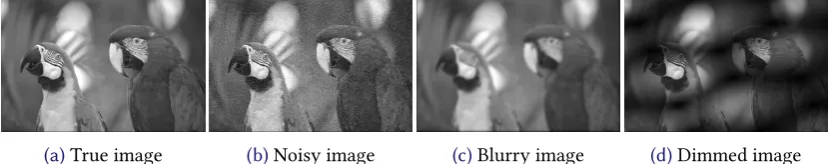
(a)True image (b)Noisy image (c)Blurry image (d)Dimmed image
Figure 1:Sample images for denoising, deblurring, and undimming experiments.
Lemma 4.4showsη2
i ≥ bminjϕj,i for someb. Thereforeη2N ≥bϕ0+bγÍiN=−01ηi. Otherwise written this saysη2
N ≥eη
2
N, where
e
η2
N =bϕ0+bγ N−1
Õ
i=0
e
ηi =eη
2
N−1+c2γeηN−1 =eη
2
N−1+bγeη
−1 N−1.
This impliesηi ≥ eηi ≥c
0
ηifor somecη0 > 0; cf. the estimates for the acceleration rule (2.3) in [6,33]. We now work through the proof ofTheorem 4.5withp =1/2 andρj =0, but using in (4.15) and (4.16) the estimateηi ≥cη0ithat would otherwise correspond top=1. Remark 4.10 (Linear rates under full primal-dual strong convexity). If bothGandF∗are strongly convex, fixingτj,i ≡τj, it is possible to derive linear rates.
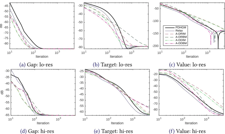
5 numerical experience
We now apply several variants of the proposed algorithms to image processing problems. We consider discretisations, as our methods are formulated in Hilbert spaces, but the space of functions of bounded variation—where image processing problems are typically formulated—is only a Banach space. Our specific example problems will be TGV2denoising, TV deblurring,
and TV undimming.
We present the corrupt and ground-truth images inFigure 1, with values in the range[0,255].
We use the images both at the original resolution of 768×512, and scaled down to 192×128
pixels. To the noisy high-resolution test image inFigure 1b, we have added Gaussian noise with standard deviation 29.6 (12dB). In the downscaled image, this becomes 6.15 (25.7dB). The image inFigure 1cwe have distorted with Gaussian blur of standard deviation 4. To avoid inverse crimes, we have added Gaussian noise of standard deviation 2.5. The dimmed image inFigure 1d, we have distorted by multiplying the image with a sinusoidal maskγ; seeFigure 1c. Again, we have added the small amount of noise to the blurry image.