Efficient Second-Order Shape-Constrained
Function Fitting
∗
David Durfee
†Yu Gao
†Anup B. Rao
‡Sebastian Wild
§May 30, 2019
We give an algorithm to compute a one-dimensional shape-constrained function that best fits given data in weighted-L∞ norm. We give a single algorithm that works for a variety of commonly studied shape constraints including monotonic-ity, Lipschitz-continuity and convexmonotonic-ity, and more generally, any shape constraint expressible by bounds on first- and/or second-order differences. Our algorithm computes an approximation with additive error ε in O nlogUε
time, where U
captures the range of input values. We also give a simple greedy algorithm that runs inO(n) time for the special case of unweightedL∞convex regression. These are the first (near-)linear-time algorithms for second-order-constrained function fitting. To achieve these results, we use a novel geometric interpretation of the underlying dynamic programming problem. We further show that a generalization of the corresponding problems to directed acyclic graphs (DAGs) is as difficult as linear programming.
1. Introduction
We consider the fundamental problem of finding a functionf that approximates a given set of data points (x1, y1), . . . ,(xn, yn) in the plane with smallest possible error, i.e., f(xi) shall be
close toyi (formalized below), subject to shape constraints on the allowable functions f, such as being increasing and/or concave. More specifically, we present a new algorithm that can handle arbitrary constraints on the (discrete) first- and second-order derivatives off.
When we only requiref to be weakly increasing, the problem is known as isotonic regression, a classic problem in statistics; (see, e.g., [13] for history and applications). It has more recently also found uses in machine learning [17, 16, 12].
In certain applications, further shape restrictions are integral part of the model: For example, microeconomic theory suggests that production functions are weakly increasing and concave (modeling diminishing marginal returns); similar reasoning applies to utility functions. Restrictingf to functions with bounded derivative (Lipschitz-continuous functions) is desirable to avoid overfitting [16]. All these shape restrictions can be expressed by inequalities for
∗The first author is supported in part by National Science Foundation Grant 1718533. The last author is supported by the Natural Sciences and Engineering Research Council of Canada and the Canada Research Chairs Programme.
†Georgia Institute of Technology · {ddurfee,ygao380}@ gatech.edu ‡Adobe Research · anuprao @ adobe.com
§University of Waterloo · wild @ uwaterloo.ca
first and second derivatives off; their discretized equivalents are hence amenable to our new method. Shape restrictions that we cannot directly handle are studied in [28] (f is piecewise constant and the number of breakpoints is to be minimized) and [26] (unimodalf). For a more comprehensive survey of shape-constrained function-fitting problems and their applications, see [14,§1]. Motivated by these applications, the problems have been studied in statistics (as a form of nonparametric regression), investigating, e.g., their consistency as estimators and their rate of convergence [13, 14, 4].
While fast algorithms for isotonic-regression variants have been designed [27], both [22] and [3] list shape constraints beyond monotonicity as important challenges. For example, fitting (multidimensional) convex functions is mostly done via quadratic or linear programming solvers [24]. In his PhD thesis, Balzs writes that current “methods are computationally too expensive for practical use, [so] their analysis is used for the design of a heuristic training algorithm which is empirically evaluated” [4, p. 1].
This lack of efficient algorithms motivated the present work. Despite a few limitations discussed below (implying that we do not yet solve Balzs’ problem), we give the first near-linear-time algorithms for any function-fitting problem with second-order shape constraints (such as convexity). We use dynamic programming (DP) with a novel geometric encoding for the “states”. Simpler versions of such geometric DP variants were used for isotonic regression [25] and are well-known in the competitive programming community; incorporating second-order constraints efficiently is our main innovation.
Problem definition. Given the vectors x = (x1, . . . , xn) ∈ Rn and y ∈ Rn, an error norm
d and shape constraints (formalized below), compute f = (f1, . . . , fn) satisfying the shape
constraints with minimald(f,y), i.e., we representf via its valuesfi =f(xi) at the given points.
dis usually anLp norm,d(x,y) =
P
i|xi−yi|p
1/p
; least squares (p= 2) dominate in statistics, but more general error functions have been studied for isotonic regression [23, 19, 22, 3]. We will consider the weighted L∞ norm, i.e.,d(f,y) = maxi∈[n]wi|fi−yi|, where [n] ={1, . . . , n} andw∈Rn
≥0 is a given vector of weights.
Since we are dealing with discretized functions (a vectorf), restrictions for derivativesf0
andf00 have to be discretized, as well. We define local slope and curvature as
fi0 = fi−fi−1
xi−xi−1
, (i∈[2..n]), and fi00 = f 0
i−fi0−1
xi−xi−1
, (i∈[3..n]);
the shape constraints are then given in the form of vectors f0−,f0+,f00−,f00+ of bounds for the first- and second-order differences, i.e., we define the set of feasible answers asF =f ∈ Rnf0−≤f0 ≤f0+∧f00−≤f00≤f00+ where inequalities on vectors mean the inequality on all components. The weighted-L∞ function-fitting problem with second-order shape constraints is then to find
f∗ = arg min
f∈F
max
i wi· |fi−yi|
. (1)
Often, we only need a lower resp. upper bound; we can achieve that by allowing−∞ and +∞ entries infi0± and fi00±. For example, settingf00−= 0,f0−=f00− = +∞ andf0−=−∞, we can enforce a convex function/vector. We also consider the decision-version of the problem: given a boundL, decide if there is anf ∈F with maxiwi|fi−yi| ≤L, and if so, report one.
1. Introduction 3
With binary search, this readily yields an additiveε-approximation for (1), and thus weighted
L∞ isotonic regression, convex regression and Lipschitz convex regression, inO nlogUεtime (Theorem 1.4), whereU = (maxiwi)·(maxiyi−miniyi). In the appendix, we give a simple
greedy algorithm (see Theorem A.1) forunweighted (w= 1) L∞ convex regression that runs in
O(n) time. Finally, we show that a generalization of the problem to DAGs (where the applied first- and second-order difference constraints are restricted by the graph), is as hard as linear programming, see Appendix D.
Related work. Stout [27] surveys algorithms for various versions of isotonic regression; they achieve near-linear or even linear time for many error metrics. He also considers the gener-alization to any partial order (instead of the total order corresponding to weakly increasing functions). A related task is to fit a piecewise-constant function (with a prescribed number of jumps) to given data. [9, 10] solve this problem forL∞ in optimalO(nlogn) time. Since the geometric constraints are much easier than in our case, a simple greedy algorithm suffices to solve the decision version.
For more restricted shapes, less is known. [26] gives a O(nlogn) solution for unimodal regression. [1] gives anO(nlogn) algorithm for unweightedL2 Lipschitz isotonic regression and aO(npoly(logn)) time algorithm for Lipschitz unimodal regression. [24] describes (mul-tidimensional)L2 convex regression algorithms based quadratic programming. Fefferman [8] studied a closely related problem of smooth interpolation of data in Euclidean space minimizing a certain norm defined on the derivatives of the function. His setup is much more general, but his algorithm cannot find arbitrarily good interpolations (εis fixed for the algorithm). All fast algorithms above consider classes defined by constraints on thefirst derivative only, not the second derivative as needed for convexity. To our knowledge, the fastest prior solution for any convex regression problem is solving a linear program, which will imply super-linear time.
We use a geometric interpretation of dynamic-programming states and represent them implicitly. The work closest in spirit to ours is a recent article by Rote [25]; establishing the transformation of states is much more complicated in the presently studied problem, though. Implicitly representing a series of more complicated objects using data structures has been used in geometric and graph algorithms, such as multiple-source shortest paths [18] and shortest paths in polygons [5, 21, 7]. The only other work (we know of) that interprets dynamic programming geometrically is [28].
There is a rich literature on methods for speeding up dynamic programming [29, 30, 6, 11]. They involve a variety of powerful techniques such as monotonicity of transition points, quadrangle inequalities, and Monge matrix searching [2], many of which have found applications in other settings. The focus of these methods is to reduce the (average) number of transitions that a state is involved in, often fromO(n) to O(1). Therefore, their running times are lower bounded by the number of states in the dynamic programs.
1.1. Results
We formally state our theorem for the decision problem here; results for shape-constrained function fitting are obtained as corollaries. For our algorithm, the discrete derivatives (as defined above) are inconvenient because they involve the x-distance between points. We therefore
normalize allx-distances to 1 (s. t. xi =i); for the second-order constraints, this normalization
makes the introduction of an additional parameter necessary, the scaling factorsαi (see below).
Definition 1.1 (1st/2nd-diff-constrained vectors): Let n-dimensional vectors x− ≤x+
α > 0 be given. We define S ⊂ Rn to be the set of all b ∈
Rn that satisfy the following
constraints:
∀i∈[1..n] x−i ≤ bi ≤ x+i (value constraints)
∀i∈[2..n] yi− ≤ bi−bi−1 ≤ yi+ (first-order constr.) ∀i∈[3..n] zi− ≤ (bi−bi−1)−αi(bi−1−bi−2) ≤ zi+ (second-order constr.)
Moreover, we consider the “truncated problems” Sk, where Sk is the set of all b ∈Rn that
satisfy the constraints up tok (instead ofn).
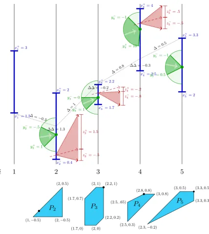
A visualization of an example is shown in Figure 1. We can encode an instance (x,y,f0±,f00±) of the decision version of the weighted-L∞function-fitting problem with second-order constraints as 1st/2nd-diff-constrained vectors by setting
x±i = yi±L/wi, y±i = f0±·(xi−xi−1),
z±i = f00±·(xi−xi−1)2, αi =
xi−xi−1
xi−1−xi−2
.
So, our goal is to efficiently compute someb∈ S or determine that S =∅. Our core technical result is a linear-time algorithm for this task:
Theorem 1.2 (1st/2nd-diff-constrained decision): With the notation of Definition 1.1, inO(n) time, we can computeb∈ S or determine that S =∅.
Section 2 will be devoted to the proof. To simplify the presentation, we will assume throughout thatx+, x−, y+, y−, z+, z− are bounded.1 For the optimization version of the problem, Equation (1), we consider approximate solutions in the following sense.
Definition 1.3 (ε-approximation): We call f ∈ F an ε-approximate solution to the weighted L∞ function-fitting problem if it satisfies
max
i wi|fi−yi| ≤ ming∈F
max
i wi|gi−yi|
+ε.
By a simple binary search onL, we can find approximate solutions.
Theorem 1.4 (Main result): There exists an algorithm that computes an ε-approximate solution to the weighted-L∞ convex regression problem that runs in O(nlogUε) time, where
U = (maxiwi)(maxiyi−miniyi).The same holds true for isotonic regression, Lipschitz isotonic
regression, convex isotonic regression.
Proof: We will argue for the case of convex regression here, other cases are similar. Abbreviate
L(f) = maxiwi|fi−yi|. For a given L, the decision version of convex regression can be solved
inO(n) time using Theorem 1.2. That is, in O(n) time, we can either findf ∈F such that
L(f) ≤L or conclude that for allf ∈F, L(f)> L. If we know an L0 for which there exists
f ∈F with L(f)≤L0, then we can do a binary search forLc in [0, L0].We can easily find such anL0 for the convex case: Let f = minyj be constant (hence convex). For this f, we have L(f)≤(maxjwj)(maxjyj−minjyj).Therefore, we can takeL0 = (maxjwj)(maxjyj−minjyj)
and the result immediately follows.
1Some problems are stated with
1. Introduction 5
1
2
3
4
5
i
x−1 = 1.5
x+ 1 = 3
x−2 = 0.4
x+ 2 = 2
x−3 = 1.7
x+ 3 = 2.2
x−4 = 2.5
x+ 4 = 4
x−
5 = 2
x+ 5 = 3.3
y−
2 =−.5
y+
2 = 1
y−3 = 0
y+
3 = 1
y4−=−1
y+
4 = 10
y−
5 =−1
y+ 5 = 0.5
z3−=−.5
z3+= 1.5
z−4 =−.8
z+
4 =−.2
z−5 =−.5
z+
5 =.5
∆= 0
.5
∆∆ =−0.3
∆=
0.8
∆∆ =−0.2
∆=
1
∆∆ = 1.3
∆ =−
0.3
(1,−0.5) (2,−0.5)
(2,0.5)
P
2(1.7,0) (2,0)
(2.2,0.2) (2.2,1) (2,1)
(1.7,0.7)
P
3(2.5,0.3)
(3,0.8) (2.8,0.8)
(2.5, .65)
P
4
(2.3,−0.2)
(3.3,0.3) (3.3,0.5) (3,0.5)
[image:5.595.80.509.97.575.2]P
5Figure 1: Exemplary input for the 1st/2nd-diff-constrained decision problem withα= 1. Value
constraints are illustrated as blue bars. First-order constraints are shown as green circles, indicating the allowable incoming angles/slopes; the green dot and the circle can be moved up and down within the blue range. Finally, second-order constraints are given as red triangles, in which the minimal and maximal allowable change in slope is shown (dotted red), based off an exemplary incoming slope (dashed red). The thin dotted line showsb= (1.7,1.2,2.2,2.8,3.3)∈ S.
Below the visualization of the instance, we show the set of pairs (bi, bi−bi−1) for
We note that for the specific case of unweighted convex function fitting, there is a simpler linear-time greedy algorithm; we give more details on that in Appendix A. This algorithm was the initial motivation for studying this problem and for the geometric approach we use. For more general settings, in particular second-order differences that are allowed to be both positive and negative, the greedy approach does not work; our generic algorithm, however, is almost as simple and efficient.
2. First- and second-order difference-constrained vectors
In this section, we present our main algorithm and prove Theorem 1.2. In Section 2.1, we give an overview and introduce the feasibility polygonsPi. Section 2.2 shows howPi can be inductively computed fromPi−1 via a geometric transformation. We finally show how this transformation can be computed efficiently, culminating in the proof of Theorem 1.2, in Section 2.3. Two proofs are deferred to Appendix B and C.
2.1. Overview of the algorithm
Recall that the problem we want to solve, in order to prove Theorem 1.2, is finding a feasible pointbinSfrom Definition 1.1. Our algorithm will use dynamic programming (DP) where each state is associated with the feasiblebi in the truncated problem. We will iteratively determine
allbi such thatbi is theith entry of someb∈ Si.
Feasible bi have to respect the first- and second-order difference constraints. To check those, we also need to know the possible pairs (bi−1, bi−2) of (i−1)th and (i−2)th entries for someb∈ Si−1, so the states have to maintain more information than thebi alone. It will
be instrumental torewrite this pair as (bi−1, bi−1−bi−2), the combination of valid valuesbi−1 and validslopes at which we enteredbi−1 for a solution inSi−1. From that, we can determine the valid slopes at which we canleave bi−1 using our shape constraints. We thus define the feasibility polygons
Pi = (x, y)∃b∈ Si:x=bi∧y=bi−bi−1 (2)
fori= 2, . . . , n. See Figure 1 for an example. We view each point in Pi as a “state” in our
DP algorithm, and our goal becomes to efficiently compute Pi fromPi−1. The key observation is that eachPi is indeed an O(n)-vertex convex polygon, and we only need an efficient way to compute thevertices of Pi from those ofPi−1. This needs a clever representation, though, since all vertices can change when going from Pi−1 to Pi. A closer look reveals that we can represent the vertex transformationsimplicitly, without actually updating each vertex, and we can combine subsequent transformations into a single one. More specifically, if we consider the boundary ofPi−1, the transformation toPi consists of two steps: (1) a linear transformation for the upper and lower hull ofPi−1, and (2) a truncation of the resulting polygon by vertical and horizontal lines (i.e., an intersection of the polygon and a half-plane).
The first step requires a more involved proof and uses that all line segments of Pi have weakly positive slope (“+sloped”, formally defined below). Implicitly computing the first
transformation as we move betweenPi is straightforward, only requiring a composition of linear
operations (a different one, though, for upper and lower hull). We can apply the cumulative transformation whenever we need to access a vertex.
2. First- and second-order difference-constrained vectors 7
increasingx-coordinate; sincePi is +sloped,y-values are also increasing. A linear search for
intersections has overallO(n) cost since we can charge individual searches to deleted vertices. Finally, if Pn6=∅, we compute a feasible vector bbackwards, starting from any point in Pn. Since we do not explicitly store thePi, this requires successively “undoing” all operations (going fromPi back to Pi−1); see Appendix C for details.
2.2. Transformation from state Pi−1 to Pi
We first define the structural property “+sloped” that our method relies on.
Definition 2.1 (+sloped): We say a polygonP ⊆R2 with vertices v1, . . . , vk is +sloped if
slope(vi, vj) ≥0 for all edges (vi, vj) of P. Here, the slope between two points v1 = (x1, y1),
v2 = (x2, y2) ∈ R2 is defined as slope(v1, v2) = x2y2−−y1x1, when x1 6= x2, and slope(v1, v2) =∞,
otherwise.
We will now show thatPi can be computed by applying a simple geometric transformation to
Pi−1. In passing, we will prove (by induction on i) that allPi are +sloped. For the base case,
note thatP2 ={(b2, b2−b1) |x−1 ≤b1 ≤x+1 ∧x −
2 ≤b2 ≤x+2 ∧y −
2 ≤b2−b1 ≤y2+}, which is an intersection of 6 half-planes. The slopes of the defining inequalities are all non-negative or infinite, soP2 is +sloped.
Let us now assume thatPi−1,i≥3, is +sloped; we will consider the transformation from
Pi−1 toPi and show that it preserves this property. We begin by separating the transformation fromPi−1 toPi into two main steps.
Step 1: Second-order constraint only. For the first step, we ignore the value and first-order constraints at indexi. This will yield a convex polygon, Pi(z), that contains Pi; in Step 2, we
will add the other constraints atito obtain Pi itself.
Definition 2.2 (Pi(z): 2nd-order-only polygons): For a fixedi, consider the modified prob-lem withx−i , y−i =−∞ andx+i , yi+ =∞. Define the second-order-only polygon, Pi(z), as the polygonPi of this modified problem (considering only the zi constraints ati).
The statement of the following lemma is very simple observation, but allows us to compute
Pi(z) fromPi−1 with an explicit geometric construction, (whereas such seemed not obvious for the original feasibility polygons).
Lemma 2.3 (P(z)
i : scaled, sheared and shifted Pi−1): Pi(z) =(x+αiy+z, αiy+z)|(x, y)∈Pi−1, z∈[zi−, zi+] .
Proof: The only constraint at iis zi− ≤(bi−bi−1)−αi(bi−1−bi−2) ≤z+i . We rewrite this as (a) a constraint forbi−bi−1, using that bi−1−bi−2 is they-coordinate inPi−1, and (b) a constraint forbi, using that, additionally,bi−1 is the x-coordinate inPi−1.
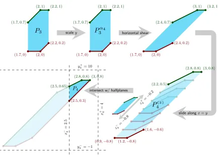
Once we have computed this polygon Pi(z), computing Pi is easy: adding the constraints x−i ≤x≤x+i andyi−≤y≤yi+requires only cuttingPi(z) with two horizontal and vertical lines. We give a visual representation of the mapping on an example in Figure 2. We break the above mapping into two simpler stages:
Corollary 2.4 (Pi(z): sheared and shifted Pαi
i−1):
SettingPαi
i−1 ={(x, αiy)|(x, y)∈Pi−1}, we have
Pi(z) =
(x+y+z, y+z)|(x, y)∈Pαi
i−1, z∈[z −
i , z
+
i ] .
(1.7,0) (2,0)
(2.2,0.2) (2.2,1) (2,1)
(1.7,0.7)
P
3 scaley(1.7,0) (2,0)
(2.2,0.2) (2.2,1) (2,1)
(1.7,0.7)
P
α43 horizontal shear
(1.7,0) (2,0)
(2.4,0.2)
(3.2,1) (3,1)
(2.4,0.7)
slide alongx=y
z
− 4
=− 0.8
z
+ 4
=− 0.2
(0.9,−0.8) (1.2,−0.8)
(1.6,−0.6)
(3,0.8) (2.8,0.8)
(2.2,0.5)
P
(z)4 (2.5,0.3)
(3,0.8) (2.8,0.8)
(2.5,0.65)
P4 x − 4 = 2 . 5 x + 4 = 4 y− 4 =−1
y+ 4 = 10
[image:8.595.79.513.84.397.2]intersect w/ halfplanes
Figure 2: The transformation from P3 to P4 for the example instance of Figure 1. Upper and
lower hull are shown separately in green resp. red.
Lemma 2.5: Letα≥0. IfP is +sloped, so is Pα ={(x, αy)|(x, y∈P)}.
Proof: Scaling they-coordinates will preserve all of the vertices ofP, and also scale the slope
of each vertex pair byα≥0. So, Pα is +sloped.
That leaves us with the core of the transformation, from Pαi
i−1 toP
(z)
i . Intuitively, it can be
viewed as sliding Pαi
i−1 along the linex=y by any amountz∈[z −
i , z
+
i ] and taking the union
thereof, (see Figure 2). To compute the result of this operation, we split the boundary into upper and lower hull.
Definition 2.6 (Upper/lower hull): Let P be a convex polygon with vertex set V. We define the upper hull (vertices) resp. lower hull (vertices) of P as
u-hull(P) = ui= (xi, yi)∈V @(xi, y)∈P :y > yi
l-hull(P) = ui= (xi, yi)∈V @(xi, y)∈P :y < yi
Unless specified otherwise, hull vertices are ordered by increasingx-coordinate.
Note that a vertex can be in both hulls. Moreover, the leftmost vertices in u-hull(P) and l-hull(P) always have the samex-coordinate, similarly for the rightmost vertices. As proved in
Lemma 2.3, each point in Pαi
2. First- and second-order difference-constrained vectors 9
Definition 2.7 (2nd-order P transform): Letfi((x, y))be the line-segment{(x+y+z, y+
z)|z∈[zi−, zi+]} and denote by fi−((x, y)) = (x+y+zi−, y+zi−) and fi+((x, y)) = (x+y+
zi+, y+zi+) the two endpoints of fi((x, y)).
We writef(S) =S
(x,y)∈Sf((x, y))for the element-wise application off to a setS of points.
The vertices of Pi(z) result from transforming the upper hull ofPαi
i−1 byf +
i and the lower hull
byfi−. The next lemma formally establishes that applying fi+ resp. fi− to the hulls ofPαi
i−1 correctly computesPi(z), (again, compare Figure 2).
Lemma 2.8 (From Pαi
i−1 to P (z)
i via hulls): If P
αi
i−1 is +sloped, then P
(z)
i is +sloped
and u-hull(Pi(z)) = {f
−
i (vll)} ∪f
+
i (u-hull(P αi
i−1)) and l-hull(P
(z) i ) = f
−
i (l-hull(Pi−1))∪
{fi+(vur)}, wherevll (lower-left) and vur (upper-right) are the first vertex ofl-hull(Piα−i1) and
the last vertex of u-hull(Piα−i1), respectively.
We defer the formal proof to Appendix B. Intuitively, since each point in Pαi
i−1 is mapped to a line-segment with slope 1 inPi(z),Pi(z) is obtained by slidingPαi
i−1 along the linex=y. Note here that we could allowzi−=−∞and/or zi+=∞, where the functionsfi−, fi+ would instead map to the ray centered at (x, x+y) and either pointed upwards or downwards with slope 1. The full transformation from Pi−1 toPi(z) can now be stated as:
Lemma 2.9 (Pi−1 to Pi(z)): Let f
∗,αi
i be the function f
∗,αi
i (x, y) = (x+αiy+zi∗, αiy+zi∗)
for∗ ∈ {−,+}. IfPi−1 is +sloped, then Pi(z) is+slopedwith
u-hull(Pi(z)) =
f−,αi
i (vll) ∪fi+,αi(u-hull(Pi−1))
l-hull(Pi(z)) = f−,αi
i (l-hull(Pi−1))∪
f+,αi
i (vur)
with vll and vur the lower-left resp. upper-right vertex ofPi−1.
Proof: This follows immediately from Corollary 2.4 and Lemmas 2.5 and 2.8.
Step 2: Truncating by value and slope. To complete the transformation, we need to add the constraints x−i ≤bi ≤x+i and y−i ≤bi−bi−1 ≤yi+ to Pi(z). This is equivalent to cutting our polygon with two vertical and horizontal planes. The following lemma shows that this preserves the +sloped-property.
Lemma 2.10 (# new vertices): IfPi−1 is+slopedwithkvertices, thenPi is either empty
or+slopedwith at most k+ 6vertices.
It follows that over the course of the algorithm, onlyO(n) vertices are added in total. This will be instrumental for analyzing the running time.
Proof: We know thatPi(z) is +sloped, and it follows easily from the definition that cutting
by horizontal and vertical planes will preserve this property. Furthermore, note that cutting a convex polygon will increase the total number of vertices by at most one. We added at most 2 vertices to Pi−1 to obtain Pi(z). We then cut P
(z)
i by the inequalitiesx≤x
+
i ,x≥x
−
i ,y≤y
−
i ,
andy≥y+i , i.e., two horizontal and vertical planes. Each adds at most one vertex, giving the
2.3. Algorithm
A direct implementation of the transformation of Lemma 2.9 yields a “brute force” algorithm that maintains all vertices ofPiand checks ifPnis empty; (the running time would be quadratic).
It works as follows:
1. [Init]: Compute the vertices of P2.
2. [ComputePi]: Fori= 3, . . . , n, do the following:
2.1. At step i, scale the y-coordinate of each vertex by αi.
2.2. Applyfi+ resp.fi− to each vertex, depending on which hull it is in.
2.3. Add the new vertex to u-hulland l-hull, as per Lemma 2.9.
2.4. Delete all the vertices outside [x−i , x+i ]×[yi−, yi+] and
add the vertices created by intersecting with [x−i , x+i ]×[y−i , yi+].
3. [Computeb]: IfPn6=∅, compute (b1, . . . , bn) by backtracing.
Observe that Lemma 2.9 applies thesame linear function (multiplication ofy-coordinate by
αi and fi+ orf
−
i ) to all vertices in u-hull resp.l-hull. So, we do not need to modify every
vertex each time; instead, we can store – separately for u-hull andl-hull – the composition
of the linear transformations as a matrix. Whenever we access a vertex, we take the unmodified vertex and apply the cumulative transformation in O(1) time.
At each step, after applying the linear transformations, by Lemma 2.9 we also need to copy the leftmost vertex of l-hull, add it to the left of u-hulland copy the rightmost vertex of u-hulland add it to the right of l-hull. To add these vertices, we simply apply the inverse
of each respective cumulative transformation such that all stored vertices require the same transformation. This will also takeO(1) time.
Since all the slopes of Pi(z) are non-negative (+sloped) and we keep vertices sorted by
x-coordinate, the truncation by a horizontal or vertical plane can only remove a prefix or suffix fromu-hullandl-hullofPi(z). Depending on the constraint we are adding, (x≤x
+
i ,x≥x
−
i , y≤yi−, ory≥yi+), we start at the rightmost or leftmost vertex of theu-hullandl-hull, and
continue until we find the intersection with the cutting plane. We remove all visited vertices. This could take O(n) time in any single iteration, but the total cost over all iterations is
O(n) since we start withO(1) vertices and addO(n) vertices throughout the entire procedure (by Lemma 2.10). This allows us to use two deques (double-ended queues), represented as arrays, to store the vertices ofu-hull andl-hull. Putting this all together gives the linear
time algorithm for the decision problem “S =∅?”.
To compute an actual solution when S 6= ∅, we compute bn, . . . , b1, in this order. From the lastPn, we can find a feasiblebn (the x-coordinate of any point in Pn). Then, we retrace the steps of our algorithm through specific points in eachPi. Since intermediate Pi were only
implicitly represented, we have to recoverPi by “undoing” the algorithm’s operations in reverse
order; this is possible in overall timeO(n) by remembering the operations from the forward phase. The details on the backtracing step are deferred to Appendix C, where we also present the final algorithm.
3. Conclusion
References 11
additionally satisfies inequalities on its first- and second-order (successive) differences. This method can be used to approximate weighted-L∞ shape-restricted function-fitting problems, where the shape restrictions are given as bounds on first- and/or second-order differences (local slope and curvature).
This is a first step towards much sought-after efficient methods for more general convex regression tasks. A main limitation of our approach is the restriction to one-dimensional problems. We show in Appendix D that a natural extension of the problem studied here to directed acyclic graphs is already as hard as linear programming, leaving little hope for an efficient generic solution. This is in sharp contrast to isotonic regression, where similar extensions to arbitrary partial orders do have efficient algorithms (forL∞) [27]. This might also be bad news for multidimensional regression with second-order constraints, since higher dimensions entail, among other complications, a non-total order over the inputs.
A second limitation is theL∞error metric, which might not be adequate for all applications. We leave the question whether similarly efficient methods are also possible for other metrics for future work. A further extension to study is convexunimodal regression; here, finding the maximum is part of the fitting problem, and so not directly possible with our presented method.
Acknowledgments
We thank Richard Peng, Sushant Sachdeva, and Danny Sleator for insightful discussions, and our anonymous referees for further relevant references and insightful comments that significantly improved the presentation.
References
[1] Pankaj K. Agarwal, Jeff M. Phillips, and Bardia Sadri. Lipschitz unimodal and isotonic regression on paths and trees. In LATIN 2010: Theoretical Informatics, pages 384–396. Springer Berlin Heidelberg, 2010. doi:10.1007/978-3-642-12200-2\_34.
[2] Alok Aggarwal, Maria M. Klawe, Shlomo Moran, Peter Shor, and Robert Wilber. Geometric applications of a matrix-searching algorithm. Algorithmica, 2(1-4):195–208, November 1987. doi:10.1007/bf01840359.
[3] Francis Bach. Efficient algorithms for non-convex isotonic regression through submodular optimization. In S. Bengio, H. Wallach, H. Larochelle, K. Grauman, N. Cesa-Bianchi, and R. Garnett, editors,Advances in Neural Information Processing Systems 31, pages 1–10. Curran Associates, Inc., 2018.
[4] G´abor Bal´azs. Convex Regression: Theory, Practice, and Applications. PhD thesis, 2016.
doi:10.7939/R3T43J98B.
[5] Bernard Chazelle. A theorem on polygon cutting with applications. In Symposium on Foundations of Computer Science (SFCS), pages 339–349. IEEE, 1982. doi:10.1109/ SFCS.1982.58.
[7] Jeff Erickson. Shortest homotopic paths, 2009. Lecture notes for computational topology. URL: http://jeffe.cs.illinois.edu/teaching/comptop/2009/notes/ shortest-homotopic-paths.pdf.
[8] C. Fefferman. Smooth interpolation of data by efficient algorithms. In Excursions in Harmonic Analysis, Volume 1, pages 71–84. Birkh¨auser Boston, November 2012. doi: 10.1007/978-0-8176-8376-4\_4.
[9] Herv´e Fournier and Antoine Vigneron. Fitting a step function to a point set. Algorithmica, 60(1):95–109, July 2009. doi:10.1007/s00453-009-9342-z.
[10] Herv´e Fournier and Antoine Vigneron. A deterministic algorithm for fitting a step function to a weighted point-set. Information Processing Letters, 113(3):51–54, February 2013.
doi:10.1016/j.ipl.2012.11.003.
[11] Zvi Galil and Raffaele Giancarlo. Speeding up dynamic programming with applications to molecular biology. Theoretical Computer Science, 64(1):107–118, apr 1989. doi: 10.1016/0304-3975(89)90101-1.
[12] Ravi Sastry Ganti, Laura Balzano, and Rebecca Willett. Matrix completion under monotonic single index models. In C. Cortes, N. D. Lawrence, D. D. Lee, M. Sugiyama, and R. Garnett, editors, Advances in Neural Information Processing Systems 28, pages 1873–1881. Curran Associates, Inc., 2015.
[13] Piet Groeneboom and Geurt Jongbloed. Nonparametric estimation under shape constraints, volume 38. Cambridge University Press, 2014.
[14] Adityanand Guntuboyina and Bodhisattva Sen. Nonparametric shape-restricted regression.
Statistical Science, 33(4):568–594, November 2018. doi:10.1214/18-sts665.
[15] Alon Itai. Two-commodity flow. Journal of the ACM (JACM), 25(4):596–611, 1978.
[16] Sham M Kakade, Varun Kanade, Ohad Shamir, and Adam Kalai. Efficient learning of generalized linear and single index models with isotonic regression. In J. Shawe-Taylor, R. S. Zemel, P. L. Bartlett, F. Pereira, and K. Q. Weinberger, editors, Advances in Neural Information Processing Systems 24, pages 927–935. Curran Associates, Inc., 2011.
[17] Adam Tauman Kalai and Ravi Sastry. The isotron algorithm: High-dimensional isotonic regression. In Annual Conference on Learning Theory (COLT), 2009.
[18] Philip N Klein. Multiple-source shortest paths in planar graphs. InSymposium on Discrete Algorithms (SODA), pages 146–155. SIAM, 2005.
[19] Rasmus Kyng, Anup Rao, and Sushant Sachdeva. Fast, provable algorithms for isotonic regression in all lp-norms. In C. Cortes, N. D. Lawrence, D. D. Lee, M. Sugiyama, and R. Garnett, editors, Advances in Neural Information Processing Systems 28, pages 2719–2727. Curran Associates, Inc., 2015.
[20] Rasmus Kyng and Peng Zhang. Hardness results for structured linear systems. In
Symposium on Foundations of Computer Science (FOCS), pages 684–695, 2017. Available at: https://arxiv.org/abs/1705.02944.
References 13
[22] Cong Han Lim. An efficient pruning algorithm for robust isotonic regression. In S. Bengio, H. Wallach, H. Larochelle, K. Grauman, N. Cesa-Bianchi, and R. Garnett, editors,Advances in Neural Information Processing Systems 31, pages 219–229. Curran Associates, Inc., 2018.
[23] Ronny Luss and Saharon Rosset. Generalized isotonic regression.Journal of Computational and Graphical Statistics, 23(1):192–210, January 2014. doi:10.1080/10618600.2012. 741550.
[24] Rahul Mazumder, Arkopal Choudhury, Garud Iyengar, and Bodhisattva Sen. A com-putational framework for multivariate convex regression and its variants. Journal of the American Statistical Association, pages 1–14, January 2018. doi:10.1080/01621459. 2017.1407771.
[25] G¨unter Rote. Isotonic regression by dynamic programming. In Jeremy T. Fineman and Michael Mitzenmacher, editors, Symposium on Simplicity in Algorithms (SOSA 2019), volume 69 ofOASIcs, pages 1:1–1:18. Schloss Dagstuhl–Leibniz-Zentrum fuer Informatik, 2018. doi:10.4230/OASIcs.SOSA.2019.1.
[26] Quentin F. Stout. Unimodal regression via prefix isotonic regression. Computational Statistics & Data Analysis, 53(2):289–297, December 2008. doi:10.1016/j.csda.2008. 08.005.
[27] Quentin F. Stout. Fastest isotonic regression algorithms, 2014. URL:http://web.eecs. umich.edu/~qstout/IsoRegAlg.pdf.
[28] Charalampos E. Tsourakakis, Richard Peng, Maria A. Tsiarli, Gary L. Miller, and Russell Schwartz. Approximation algorithms for speeding up dynamic programming and denoising aCGH data. Journal of Experimental Algorithmics, 16:1.1, May 2011. doi:10.1145/ 1963190.2063517.
[29] F. Frances Yao. Efficient dynamic programming using quadrangle inequalities. In Sympo-sium on Theory of Computing (STOC). ACM Press, 1980. doi:10.1145/800141.804691.
Appendix
A. Simple greedy algorithm for convex regression
In this appendix, we give details on a simpler algorithm for the special case of unweighted convex function fitting.
Theorem A.1: There exists an algorithm for the unweightedL∞ convex regression that runs
inO(n) time.
Proof: We consider the following problem. Given ann-dimensional vectora, and parameter ∆≥0, find a convex vectorbsuch thatkb−ak∞≤∆, if such a vector exists.
This clearly fits under our parameters of Definition 1.1 by setting x− =a−∆,x+ =a+ ∆, bothy− andy+ to be unbounded, andz− = 0,z+ =∞, along withα= 1. A binary search on ∆ gives aO(nlogUε) algorithm.
However, this can also be solved by considering the set of points (i, ai+ ∆) for alli, and
taking the lower hull,2 H(∆), such that for each point (i, hi) in this lower hull we setbi =hi. We claim that the minimum possible ∆ such thatbi ≥ai−∆ is exactly the answer to this problem. If (i, ai+ ∆) is a vertex of the convex hull, bi = ai+ ∆ is always at least ai−∆.
Otherwise, let (j, aj+ ∆), (k, ak+ ∆) be two vertices of H such thatj < i < k. We have
bi ≥ ai−∆
⇐⇒ aj+ ∆ +
ak−aj
k−j (i−j) ≥ ai−∆
⇐⇒ ∆ ≥ 1 2
ai−aj+ i−j
k−j(ak−aj)
If ∆ violates this for some i, j, k, then it is impossible to fit a convex function through the intervals [(j, aj−∆),(j, aj+ ∆)], [(i, ai−∆),(i, ai+ ∆)], and [(k, ak−∆),(k, ak+ ∆)].
Conversely, if ∆ satisfies all of such constraints, bi≥ai−∆ for all 1≤i≤n, thenbi cannot be greater thanai+ ∆ as that would violate H being the convex lower hull of (i, ai+ ∆). Thus, (b1, . . . , bn) is a possible solution.
It takesO(n) time to compute the lower convex hull andO(n) time to calculate the minimum ∆. Thus, this algorithm solves L∞ convex regression inO(n) time.
The above method can also be adapted for inputs withx-values that are non-uniformly spaced. However, it does not directly generalize to weightedL∞regression: moving points up by wi·∆ can lead to different lower hulls for different values of ∆.
2The lower hull of a set of points is the subset of vertices (x
i, yi) of the convex hull, whereyiis the minimal
B. Proof of Lemma 2.8 15
B. Proof of Lemma 2.8
The proof of Lemma 2.8 will be separated into two stages. First, we show that the polygon defined by{fi+(u-hull(Piα−i1))} ∪{f
−
i (l-hull(P αi
i−1))}has upper-hull{f −
i (vll), f
+
i (u-hull(P αi
i−1))}and lower-hull{fi−(l-hull(Piα−i1)), f
+
i (vur)}, wherevll is the first vertex ofl-hull(Piα−i1) andvur is the last vertex ofu-hull(Piα−i1). Furthermore, this polygon will have slopes between vertices in [0,1]. This property will then allow us to show thatPi(z) is equivalent to the convex hull of the vertices, which implies the claim.
In order to show that the Pi(z) has all slopes between 0 and 1, we consider howfi− and fi+
affect slopes.
Lemma B.1 (Bounded slopes): IfP is+sloped, then for any connected verticesvj, vk∈V,
any i, and ∗ ∈ {−,+}, we have
0≤slope(fi∗(vj), fi∗(vk))≤1
and for any connected vertices vj, vk, vl ∈V, if slope(vj, vk)<slope(vk, vl), then
slope(fi∗(vj), fi∗(vk))<slope(fi∗(vk), fi∗(vl))
Proof: We first write the slope function explicitly to obtain
slope(fi∗(vj), fi∗(vk)) =
(yj+zi∗)−(yk+zi∗)
(xj+yj+zi∗)−(xk+yk+zi∗)
= yj−yk (xj−xk) + (yj−yk)
.
This implies that if slope(vj, vk) =∞ then slope(fi∗(vj), fi∗(vk)) = 1, and if slope(vj, vk) = 0
then slope(fi∗(vj), fi∗(vk)) = 0. Furthermore, this gives the identity
slope(fi∗(vj), fi∗(vk))−1 = slope(vj, vk)−1+ 1
when slope(vj, vk)∈(0,∞).Combined with the fact that all slopes are non-negative, this gives
both of our desired inequalities.
The first inequality of the lemma above will allow us to show that all of the slopes between vertices are bounded, and the second implies that each of the vertices remains a vertex, giving the following corollary.
Corollary B.2 (Hulls by elementwise transformation):
IfPαi
i−1 is+sloped, then the convex hullP of V =f +
i (u-hull(P αi
i−1))∪f −
i (l-hull(P αi
i−1)) has
u-hull(P) = {fi−(vll), fi+(u-hull(P αi
i−1))} and l-hull(P) = {f −
i (l-hull(P αi
i−1)), f +
i (vur)},
where vll is the first (lower-left) vertex of l-hull(Piα−i1) and vur is the last (upper-right)
vertex of u-hull(Piα−i1). Furthermore, for any connected vertices vj, vk in P, we have 0 ≤
slope(vj, vk)≤1.
Proof: By construction, the first and last vertices ofu-hull(P) andl-hull(P) are the same.
Letvu1 be the first vertex ofu-hull(Piα−i1), which gives two possibilities, either (1): vu1 =vll,
or (2) slope(vu1, vll) = ∞. For case (1) it is easy to see that slope(fi+(vu1), fi−(vll)) = 1,
and for case (2), we showed in the proof of Lemma B.1 that slope(vu1, vll) = ∞
im-plies slope(fi+(vu1), fi+(vll)) = 1, which combined with slope(fi+(vll), fi−(vll)) = 1 gives
slope(fi+(vu1), fi−(vll)) = 1. Furthermore the slopes between all vertices in u-hull(Piα−i1) are less than ∞ by Definition 2.6, and therefore less than 1 under the transformation by Lemma B.1. Along with the second inequality of Lemma B.1, this implies thatu-hull(P)
By symmetric reasoning we see that l-hull(P) makes up a convex function from
fi−(vll) to fi+(vur). Additionally, the second inequality states that every element in
{fi−(l-hull(Piα−i1)), fi+(vur)} and{fi−(vll), fi+(u-hull(P αi
i−1))} must be a vertex. Accordingly,
P must be a convex polygon with all slopes between 0 and 1. We now have fixed upper and lower hulls of a polygon, and we use the representation as the convex hull its vertices, along with the bounded-slope property, to show that this polygon is in fact equal toPi(z). In particular, all the slopes being bounded by 1 will be critical here because each point (x, y)∈Pαi
i−1 maps to a line segment from (x+y+z −
i , y+z
−
i ) to (x+y+z+i , y+z+i ),
which has slope 1. If we then consider (x, y) to be in the upper hull, if the slopes of our new upper-hull forPi(z) were greater than 1, the point (x+y+z−i , y+zi−) would lie outside of this hull. Our bounded slopes prevent this, though, and lead to the following lemma.
Lemma B.3: LetPαi
i−1 be +sloped and letP be the convex hull of
V = fi+(u-hull(Pαi
i−1)) ∪
fi−(l-hull(Pαi
i−1)) .
Then P =Pi(z).
Proof: We show both inclusions.
• P ⊆Pi(z).
By definition ofP, any point u∈P, can be written as a convex combination
X
(xj,yj)∈V(Piαi−1)
pj((xj+yj, yj) + (z∗i, zi∗)),
where the sum is over the vertices (xj, yj) ofPiα−i1, ∗ ∈ {−,+}, and P
pj = 1. We set
z = P
pjzi∗; clearly, z ∈ [zi−, z+i ]. Furthermore set x = P
pjxi and y = P
pjyj. We
know each (xj, yj) is a vertex inPiα−i1, so by convexity (x, y) must be inP
αi
i−1, implying (x+y+x, y+z)∈Pi(z) by Corollary 2.4.
• Pi(z) ⊆P.
Assume towards a contradiction there were (x+y+z, y+z)∈Pi(z) with (x, y)∈Pαi
i−1and
z∈[zi−, zi+], but (x+y+z, y+z)∈/P. By definition and assumption, both P andPαi
i−1 are convex, so there must be avertex (xv, yv) ofPiα−i1 such that (xv+yv+z, yv+z)∈/ P. Furthermore, by convexity of P, there must also exist z ∈ {zi−, z+i } such that (xv+yv+z, yv+z)∈/ P. Assume w. l.o.g. that (xv, yv)∈u-hull(Pαi
i−1). By definition of
P, we have (xv+yv+zi+, yv+zi+)∈P, so we must have z=z
−
i .
SincePαi
i−1is +slopedandfi is monotone,fi−(vll) is dominated3by (xv+yv+zi−, yv+z−i ),
and similarly,fi+(vur) dominates (xv+yv+zi−, yv+zi−). Furthermore, by Corollary B.2
the upper hull lies above the line segment from fromfi−(vll) to (xv+yv+zi+, yv+z
+
i ) and
has slope at most 1. But the slope between (xv+yv+zi−, yv+zi−) and (xv+yv+z+i , yv+z+i )
is exactly 1, so (xv+yv+z−i , yv+zi−) cannot lie above the upper hull.
Finally, (xv + yv +z−i , yv +zi−) also cannot lie below l-hull(P) because otherwise
there would exist (xv, y)∈Pαi
i−1 that lies above (xv, yv), contradicting (xv, yv) being in
u-hull(Piα−i1). Because the upper hull and lower hull combine to the convex polygon P and because thex-coordinate of (xv+yv+zi−, yv+zi−) is within the range ofx-coordinate
ofP, we have (xv+yv+zi−, yv+zi−)∈P, a contradiction. With this, we finish the proof of our lemma.
Proof of Lemma 2.8: Follows directly from Corollary B.2 and Lemma B.3.
3(x
C. Complete algorithm 17
C. Complete algorithm
In this appendix, we give detailed pseudocode for our entire algorithm. We also discuss the details on the backtracing step, i.e., computing an actual solutionb∈ S from the (implicitly represented) feasibility polygonsP2, . . . , Pn. The final procedure is shown in Algorithm 1.
C.1. Implicitly computing the Pi
The main ideas have been described in Section 2.3. We represent points in homogeneous coordinates, i.e., (x, y) becomes the column vector (x, y,1)T. That allows our transformation to be represented as a single matrix, and we can compose them by multiplying the matrices. We store the current matrix in Algorithm 1 inSu (for the upper hull) andSv for the lower hull. u andv denote the deques storing the (untransformed) points ofu-hull andl-hull in
homogeneous coordinates and in sorted order.
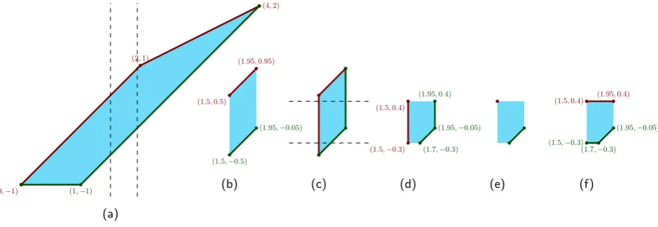
To compute Pi from Pi−1 (Step 2), we update the transformation matrices and add the new points to the hull (following Lemma 2.9). After that (line 9), u and v represent Pi(z). To implement the intersection with the half planes corresponding to the value and first-order constraints at i, we separately cut upper and lower hull with all four boundaries. Since we store upper and lower hull separately, vertical line segments are not explicitly represented in either hull, which requires some care in cutting with horizontal lines. We therefore use the following strategy –it is illustrated on an example in Figure 3: We first cut with the left and right boundaries (the value constraints), then transform our representation temporarily to left and right hulls (lines 17–18), which can easily handle cutting by horizontal line segments. Cutting is always implemented as a linear scan ofu resp.v, during which all vertices outside the constraint halfplane are removed. Then we add a new vertex at the intersection of the last segment with the constraint. (We remember the last removed vertexr for doing so.)
(0,−1)
(2,1)
(4,2)
(1,−1)
(a)
(1.5,0.5)
(1.95,0.95)
(1.5,−0.5)
(1.95,−0.05)
(b) (c)
(1.5,−0.3) (1.5,0.4)
(1.7,−0.3) (1.95,−0.05) (1.95,0.4)
(d) (e)
(1.5,0.4) (1.95,0.4)
(1.5,−0.3) (1.7,−0.3)
(1.95,−0.05)
[image:17.595.69.539.448.610.2](f)
Figure 3: Example for lines 10–30 of Algorithm 1. (a) The polygonPi(z)(after line 9). (b) After
Algorithm 1: 1st/2nd-Diff-Constrained Decision Algorithm
Input: Vectorsx−≤x+,y−≤y+,z−≤z+,α≥0
Output: Someb∈ S, orinfeasible ifS=∅.
1 Note: We represent vertex(x, y)by real vector(x, y,1)T, (homogeneous coordinates).
2 [Step 1: Init]
3 u←deque with vertices of upper hull ofP2 (sorted byx-coordinates); 4 v←deque with vertices of lower hull of P2 (sorted byx-coordinates);
5 Su←I3; Sv ←I3 ; /* init maps to the identity matrix I3 in R3×3 */ 6 [Step 2: ComputePi]
7 fori←3 tondo
8 Su←
1 αi zi+ 0 αi zi+
0 0 1
·Su; Sv ←
1 αi zi− 0 αi zi−
0 0 1
·Sv; /* Update maps */
/* Add new LL / UR vertex to hulls after transformation */
9 u.push front (Su)−1·Sv·v.front(); v.push back (Sv)−1·Su·u.back();
10 forc∈ {u, v}do/* Cut left and right boundary */ 11 r←null;whilec.size()≥1∧(Sc·c.front())x< x−i dor←Sc·c.pop front();
12 if c.empty()then returninfeasible;
13 if r6=null thenq←Sc·c.front();c.push front (Sc)−1· q+qx−x
−
i
qx−rx ·(r−q) ;
14 r←null;whilec.size()≥1∧(Sc·c.back())x> x+i dor←Sc·c.pop back(); 15 if c.empty()then returninfeasible;
16 if r6=null thenq←Sc·c.front();c.push front (Sc)−1· q+x +
i−qx
rx−qx ·(r−q) ; /* Temporarily add vertices for vertical line segments (simplifies cuts) */
17 if (Su·u.front())y>(Sv·v.front())y thenu.push front (Su)−1·Sv·v.front(); 18 if (Su·u.back())y>(Sv·v.back())y thenv.push back (Sv)−1·Su·u.back()
;
19 forc∈ {u, v}do/* Cut upper and lower boundary */ 20 r←null;whilec.size()≥1∧(Sc·c.front())y< yi− dor←Sc·c.pop front();
21 if c.empty()then returninfeasible;
22 if r6=null thenq←Sc·c.front();c.push front (Sc)−1· q+ qy−y−i
qy−ry ·(r−q) ;
23 r←null;whilec.size()≥1∧(Sc·c.back())y> y+i dor←Sc·c.pop back(); 24 if c.empty()then returninfeasible;
25 if r6=null thenq←Sc·c.front();c.push front (Sc)−1· q+y +
i−qy
ry−qy ·(r−q) ;
26 llc←Sc·c.front(); urc←Sc·c.back(); /* Store current LL/UR for later */
/* Remove generated duplicate nodes and vertical segments */ /* (sndFront/sndBack denote the second / second-to-last elements) */
27 whilec.size()≥2∧(Sc·c.front())x= (Sc·c.sndFront())xdoc.pop front(); 28 whilec.size()≥2∧(Sc·c.back())x= (Sc·c.sndBack())x doc.pop back();
/* Add stored LL/UR vertices if horizontal segments missing */
29 if (Sv·v.front())x>(Su·u.front())xthenv.push front (Sv)−1·llu
;
30 if (Su·u.back())x<(Sv·v.back())xthenu.push back (Su)−1·urv
;
31 [Step 3: Computeb]
32 (x, y)←Su·u.back(); bn ←x; p←index of the last element ofu; 33 fori←nto 3do
34 Revertu,v,Su,Sv to the previous stage;
35 x0 ←x−y;
36 whilepx< x0 dop++;
37 Useup andup−1 (if exists) to computeym←max{y0|(x0, y0)∈Pi−1}; 38 if y≥αiym+zi− then(x, y)←(x0, ym)else (x, y)←(x0,(y−z−i )/αi); 39 bi−1←x;
40 b1←x−y;
C. Complete algorithm 19
C.2. Backtracing
Suppose we have computedPn as described above, and then partially backtraced through a sequence of feasible points. We are now at (bi+1, bi+1−bi) inPi+1. Since (bi+1, bi+1−bi) = (x+ y+z, y+z),z∈[z−i+1, zi++1] for some (unknown) (x, y) = (bi, αi+1(bi−bi−1))∈Pi, we can recover x=bi from (bi+1, bi+1−bi) by subtracting the two coordinates of (bi+1, bi+1−bi). To recover
y, suppose we can find ymax= max{y|(bi, y)∈P αi+1
i } efficiently. Since {y|(bi, y)∈P αi+1 i }is
an interval, the following lemma allow us to findbi−bi−1.
Lemma C.1 (back 1 step): Let fi+1(x, y) = {(x+y+z, y+z) |z ∈ [zi−+1, zi++1]}. Either (bi+1, bi+1−bi)∈fi+1((bi, ymax))or(bi+1, bi+1−bi) = (bi+y+zi−+1, y+z
−
i+1)for somey < ymax. Intuitively, a vertical line segmentLinsidePi is mapped to a line-segment with slope 1 inPi+1, because the line segments the points inL are mapped to lie all on the same line (overlapping with each other).
Proof: If (bi+1, bi+1−bi)6∈fi+1(bi, ymax), by the maximality ofymax,bi+1−bi< ymax+z−i+1. Since there exists (bi, y0) such that (bi+1, bi+1 −bi) ∈ fi+1(bi, y0), (bi + y0 +z, y0 +z) = (bi+1, bi+1−bi) for somez∈[zi−+1, z
+
i+1]. Considerfi+1(bi, y+z−zi−+1). Then (bi+1, bi+1−bi) =
(bi+(y0+z−zi−+1)+z−i+1,(y0+z−z−i+1)+zi−+1). Sincebi+1−bi < ymax+zi−+1,y0+z−zi−+1< ymax. The lemma is proven by letting y bey0+z−z−i+1.
In the former case of Lemma C.1, we can take (x, ymax) as (bi, αi+1(bi−bi−1)). In the latter case, we can take (bi,(bi+1−bi)−zi−+1) as (bi, αi+1(bi−bi−1)).
Since ymax is they-coordinate of the intersection ofu-hull(Pi) and the vertical line (bi,·),
to computeymax, we want to find two vertices in u-hull(Pi), (xl, yl) and (xr, yr), such that xl≤bi≤xr. (bi, ymax) is just the intersection of the line segment between (xl, yl) and (xr, yr) and the vertical line (bi,·). The following lemma shows how to find (xl, yl) and (xr, yr) efficiently
using an amortized constant-time algorithm.
Lemma C.2 (Computingymax): Suppose (xl, yl) and (xr, yr) are two vertices in
u-hull(Pi), and some point (bi, y) ∈ Pi satisfies xl ≤ bi ≤ xr. Let (x0, y0) be some
point inPi+1 with (x0, y0)∈fi+1(bi, αi+1y). Thenx0 ≤(fi++1(xr, αi+1yr))x, where (·)x means
taking the x-coordinate of a point and (·)y takes they-coordinate.
Proof: Assume towards a contradiction that x0 >(fi++1(xr, αi+1yr))x. Since x0 −y0 = bi ≤ xr = (fi++1(xr, αi+1yr))x −(fi++1(xr, αi+1yr))y, we have y0 > (fi++1(xr, αi+1yr))y. But y0 = αi+1y+k≤αi+1y+zi++1 ≤αi+1yr+zi++1= (fi++1(xr, αi+1yr))y. Contradiction.
The amortized constant-time algorithm to retrieve (bn, . . . , b1) depends on the implementation of the deques. Since we will add n vertices to the deques during the whole algorithm, the (textbook) fixed-size array-based implementation suffices; we recall it to fix notation. A deque
dis represented by arrayA and two indices pl,pr. pl is the index of the first element ofdand pr is the index of the last element. If we want to add an element eto the left of the deque, the two operations pl ← pl−1, A[pl] = esuffice. Similarly, we can add/pop elements from
left/right. During our algorithm,pl (resp. pr) can move to the left (resp. right) by at mostn
positions, soAcan be an array of length 2n+O(1). If we store the vertices ofP2 in the middle ofA initially, we never exceed the boundaries of A when running the algorithm.
Definition C.3 (Position): We defineposi(x0)as the smallest index (in the array representing deque u) of a vertex of u-hull(Pi(·))withx-coordinate at leastx0.
Lemma C.4 (Monotonicity of positions):
posi(bi)≥posi+1(x0) for some(x0, y0)∈fi+1(bi, αi+1y).
Proof: By Lemma C.2,x0≤(fi++1(xr, αi+1yr))x. Sofi++1(xr, αi+1yr) is stored afterposi+1(x0). And since our algorithm stores fi++1(xr, αi+1yr) at the same place as (xr, yr), posi+1(x0) ≤
posi(bi).
Lemma C.4 allows us to findposi(z) by moving a pointer monotonically to the right. Thus, we can retrievebn, . . . , b1 in order by unrolling our linear algorithm for the decision problem and moving the pointerposi(z). This process takes O(n) time overall.
C.3. Analysis
We conclude with the proof of our main theorem.
Proof of Theorem 1.2: The correctness of Algorithm 1 follows from the preceding discussions: By Lemma 2.9, the iterative transformations compute thePi as defined in (2), andS 6=∅ iff
Pn 6=∅. Moreover, Lemma C.1 shows that, when S 6=∅, Step 3 computes a valid b∈ S. It
remains to analyze the running time.
• Step 1 takesO(1) time since the vertices ofP2 are a subset of the (at most) 12 intersection points of the defining lines. (P2 is the trapezoid spanned by (x−2, x
−
2 −x+1),(x − 2, x
− 2 −
x−1),(x+2, x+2 −x+1),(x2+, x+2 −x−1), intersected with the halfspacesy≥y−2 and y≤y+2.)
• Step 2. The operations inside the loops are all constant-time and the outer loop runs
O(n) times. Moreover, the inner while-loops all remove a node from a deque, so their total cost over all iterations of the for-loop is O(n), too: We start with O(1) vertices and adding at mostO(n) vertices throughout the entire procedure (Lemma 2.10), so we cannot remove more thanO(n) vertices.
• Step 3. All operations except for the first line inside the for-loop take constant time. The inner while-loop runs for overallO(n) iterations, since p only moves right and we add
O(n) vertices in total.
It remains to implement the first line of the loop body inO(n) overall time. To be able to undo the changes tou, v,Su, Sv, we keep alog for each instruction executed in Step 2, so that we can undo their changes here (in the opposite order). Since Step 2 runs inO(n) total time, the rollback also runs inO(n) time.
Since all three steps run in linear time, so does the whole algorithm.
D. Generalization to DAGs is hard
In this appendix, we will give a natural generalization of Definition 1.1 to arbitrary DAGs and investigate its complexity. Our original setting with differences of adjacent indices only corresponds to a directed-path graph.
In light of rather general results for isotonic regression, the path setting might appear quite restrictive; we will argue here why these conditions probably cannot be relaxed much further if we want an O(n) time algorithm.
Definition D.1: Suppose we are given a directed acyclic graph G = (V, E) with m = |E|
D. Generalization to DAGs is hard 21
dimensional vector y− ≤y+, andmp dimensional vectors z−≤z+ andα≥0. We define SG to
be the set of alln-dimensional vectorsbsuch thatx−i ≤bi≤x+i for alli,y
−
ij ≤bj−bi ≤yij+for all
edges(i, j)∈E, and zijk− ≤(bk−bj)−αijk(bj−bi)≤zijk+ for all pairs of edges(i, j),(j, k)∈E.
In contrast to Theorem 1.2, we show that determining if SG if empty or not is as hard as
solving linear programs.
Theorem D.2: With notation as in Definition D.1, if we can determineSG is empty or not in
timef(n+m+mp), then we can determine feasibility of any set of linear constraints defined
bys bounded integer coefficients in c1f(c2slogM)) time, wherec1 andc2 are two constants
and the absolute value of each coefficient in the linear constraints is no more than M.
Our reduction to prove Theorem D.2 is closely motivated by the hardness of isotropic total variation from [20], as well as subsequent works on extending such hardness results to positive linear programs. Compared to these results though, it sidesteps linear systems, and is a more direct invocation of the completeness of 2-commodity flow linear programs from [15].
We first consider a more restricted class of problems than Definition D.1 allows (where all theα’s in Definition D.1 are set to be 1). Formally we define the problem as:
Definition D.3: A generalized second-order constrained feasibility problem is defined by variables b1. . . bn, combined with a set of m constraints parameterized by
1. Upper and lower bounds on the variablesx−i and x+i .
2. Upper and lower bounds on the first order differences yi− and y+i and corresponding indicespi< qi.
3. Upper and lower bounds on the second order differenceszi− andz+i and corresponding indicesri< si < ti
and constraints
Value Constraints: x−i ≤bi ≤x+i
First Order Constraints: yi−≤bqi−bpi ≤y +
i
Second Order Constraints: z−i ≤(bti−bsi)−(bsi−bri)≤z +
i .
The goal is to decide whether there existsb1, . . . , bn that satisfy all these constraints
simultane-ously.
Proof of Theorem D.2: It is easy to see that the problem defined in Definition D.3 is a special case of the problem in Definition D.1. This is obtained by forming a DAG with edges (pi, qi), (ri, si), (si, ti) for all pi,qi,ri,si,ti. We will prove that a general linear programming feasibility problem with s polynomially-bounded integer coefficients can be expressed as a second-order-constrained feasibility problem (Definition D.3). In particular, we will show that a feasibility of a set of linear constraints containing at mostsnon-zero coefficients whose absolute values are integers no more than M can be reduced toO(slogM) value, first order and second order constraints as in Definition D.3.
Note that the second constraint in Definition D.3 is the same as
zi−≤2bqi−bri−bpi ≤z +
In particular, it allows us to create constraints of the form
2bqi =bpi+bri.
We will now show how we can restate a feasibility of a set of general linear constraints can be expressed as a second order constrained feasibility problem as in Definition D.1. The main idea will be clear when we consider a linear constraint of the form
bi1+bi2 +. . . bik ≤ci,
with k a power of 2, and i1 < i2 < . . . < ik in increasing order. To express this in terms of
second order constraints, we can introduce new variables
i1 < i12< i2
i3 < i34< i4
. . .
and usebi12 to represent the sum of bi1 andbi2 and so on. Repeating this halves the value ofk, but aggregates the whole sum into a single variable. Therefore, we can express the above linear constraint as one value constraint
bi12...k ≤x +
12...k :=ci
andk−1 second order constraints
bi12 =bi1 +bi2, . . . , bi(k−1)k =bik−1+bik, . . . , bi1...k =bi1...k/2+bik/2+1...k.
In casek is not a power of 2, we can add dummy variables whose values we restrict to zero using the value constraints. This process uses at mostk value constraints. So we have shown that we can express any linear constraint of the formbi1 +bi2 +. . . bik ≤ci in terms of O(k) second order constraints andO(k) value constraints.
Now consider the case with both positive and negative values in the linear constraint
bi1 ±. . .±bik ≤ci.
We can aggregate the sums of the variables with positive coefficients and negative coefficients separately, and let us denote the resulting variables by bpos, bneg. We can now bound the difference using a first order constraint of the form
bpos−bneg≤ci.
This results in additional O(1) first order constraints for each linear constraint.
Finally, when the coefficients are arbitrary integers, we can do pairing based on the binary representation. The second order constraint and value constraint allows us to create constrains of the form
0≤2bi−b0−bj ≤0
0≤b0 ≤0
which are equivalent to
bj = 2bi.
So we can introduce new variablesdkj representing 2kbj for any 1≤k≤cwherecis a constant.
D. Generalization to DAGs is hard 23
M, we first represent each coefficient by its binary representation, increasing the number of non-zero coefficients byO(logM) times and creating O(klogM) second order constraints and value constraints. Then all the coefficients in the linear constraints are +1 or −1 and we can use the reduction above. In summary, we can solve any linear programming feasibility problem with O(s) non-zero coefficients which are integers bounded by M by a generalized second-order constrained feasibility problem ofO(slogM) constraints. This together with our assumption of an algorithm solving generalized second-order constrained feasibility problem inf(·) time