The Influence of Cost Assumptions on Properties of the Combined Assignment Control Problems.

This is a repository copy of The Influence of Cost Assumptions on Properties of the Combined Assignment Control Problems..

White Rose Research Online URL for this paper: http://eprints.whiterose.ac.uk/2244/

Monograph:

van Vuren, T. (1990) The Influence of Cost Assumptions on Properties of the Combined Assignment Control Problems. Working Paper. Institute of Transport Studies, University of Leeds , Leeds, UK.

Working Paper, 314

[email protected] https://eprints.whiterose.ac.uk/

Reuse

Unless indicated otherwise, fulltext items are protected by copyright with all rights reserved. The copyright exception in section 29 of the Copyright, Designs and Patents Act 1988 allows the making of a single copy solely for the purpose of non-commercial research or private study within the limits of fair dealing. The publisher or other rights-holder may allow further reproduction and re-use of this version - refer to the White Rose Research Online record for this item. Where records identify the publisher as the copyright holder, users can verify any specific terms of use on the publisher’s website.

Takedown

If you consider content in White Rose Research Online to be in breach of UK law, please notify us by

White Rose Research Online

http://eprints.whiterose.ac.uk/

Institute of Transport Studies University of Leeds

This is an ITS Working Paper produced and published by the University of Leeds. ITS Working Papers are intended to provide information and encourage discussion on a topic in advance of formal publication. They represent only the views of the authors, and do not necessarily reflect the views or approval of the sponsors.

White Rose Repository URL for this paper: http://eprints.whiterose.ac.uk/2244/

Published paper

van Vuren, Tom (1990) The Influence of Cost Assumptions on Properties of the Combined Assignment Control Problems. Institute of Transport Studies,

University of Leeds. Working Paper 314

Working

Paper

314

October

1990

The influence of cost assumptions

on properties of the combined

assignment control problem

Tom van Vuren

ITS Working Papers are intended to provide information and encourage discussion on a topic in advance of formal publication. They represent only the views of the authors, and do not necessarily reflect the views or approval

Abstract

CONTENTS

Page

Properties of control policies that ensure an equilibrium Properties of policies with the BPR cost function

Properties of policies with Webster's cost function Properties of policies with Davidson's cost function A new pragmatic power policy

Tests on a simple network

Tests with the BPR cost function Tests with Webster's cost function Tests on more realistic networks Introduction

An adaptation of Webster's cost function A green time control algorithm

Implementation aspects of the iterative assignment control procedure

Results for the TGA network Results with the BPR cost function Results with Webster's cost function Conclusions TGA network

Results for the Weetwood network Results with the BPR cost function Results with Webster's cost function A more dynamic example

Conclusions for the Weetwood network

10. References

APPENDIX 1: Monotonicity with BPR delay function APPENDIX 2: Monotonicity with Webster's cost definition APPENDIX 3: Monotonicity with Davidson's cost function APPENDIX 4: Polynomial cost implementation

2

1 Pro~erties of control ~olicies that ensure an eauilibrium

In Smith (1981b) the following expression for Wardrop equilibrium assignment is introduced:

"more costly routes carry no flow" (1)

Just like routes consist of sets of links that can be traversed consecutively, we can envisage signal stages to consist of sets of links that may be given green time simultaneously. We can now define stage pressures Pj for all stages, which are

made up of the sum of the relevant

link

pressures pi, just like route costs are

made up of the sum of the relevant link costs,

The link pressures pi are determined by the control policy employed; they are a function of

fi

and

&

so that

and, following the same argument as in (1) we can express signal control policies as follows, subject to minimum green constraints (Smith et al., 1987):

"less pressurised stages receive no green" (4)

Link pressures would be si4 for Po and fiadja& for delay minimisation. These stage pressures are determined by a summation over all links that have green during that stage, as in (2). The exception is Webster's policy, in which the summation over links is replaced by a determination of the maximum pressurised link i in the stage; the link pressure in that case is m s i

.

The condition the flow pattern f must satisfy, at equilibrium, may be written as (Smith, 1979131

-t(P

,

h) is normal, at P, to D ( 5 )

Using the same arguments for a given control policy, to satisfy (4), green times should follow:

p(f

,

h*) is normal, at h*, to

E

₍₆₎

where E is the set of allowable green times.

The combined problem, which we investigate here, and in which we look for a set of flows and green times that satisfy (5) and (6) simultaneously, will be solved if

(-t(f

,

h)

,

p(f

,

1))

is normal, at (f

,

h) to DxE (7)

This condition (7) now enables us to investigate properties of existing control policies, but more importantly, to develop new control policies with advantageous properties, e.g. policies that ensure convergence of the iterative assignment control algorithm to a unique mutual equilibrium.

A straightforward condition on the control policy, that ensures convergence and uniqueness of the resulting equilibrium is:

(t

,

-p) is the gradient of a convex function V (8)

so that each (t,

,

-pi) must be the gradient of a convex function Vi; and V =

&

Vi

.

(ti

,

-pi) is the gradient of Vi if

and

avph

= -pi

If Vi is smooth then

aVi/af,dh, = dTA&afi

Now we can express pi as follows:

This opens a world of control policies with different characteristics. The simplest policy is the policy with = 0, so that

The policy that gives rise to this pressure definition is equivalent to an approximation to the NDP as suggested by Poorzahedy and Turnquist (1982). We will call this policy an integrable policy P,.

Although the policy P, gives rise to pressure definitions that are gradients of a function Vi, it is not certain that this function Vi is convex. However, if we allow a

@Xh)

as in (13),

we can define 4:s that render Vi convex, and thus ensure convergence of the iterative assignment control procedure. To ensure convexity of Vi, the vector pair (f

,

-pi) must be monotone, so that its symmetrized Jacobian is positive semi-definite, and @, must be chosen

to

ensure this.

The

need for the introduction of a "correction term" Qi and the actual form of it

depends on the cost assumptions in the delay curve. This will be discussed in the next Sections; we will call such adapted policies (which contain an appropriate correction term @i) PMr as they are both integrable and monotone.

2 Prouerties of policies with the BPR cost function

The so-called BPR cost function is extensively used in the USA, and has the following general form for signal-controlled links:

consisting of a free flow travel time

to

and a delay element at0(5k#.

It is shown in Appendix 1 that for this cost function, Webster's policy and Po are

policies that are not monotone, so that a unique solution to the combined signal control/assignment problem is not guaranteed.

Furthermore, the integrable policy PI turns out to be monotone; no correction term is needed and the policy P, is therefore of no relevance. For this cost function delay minimisation turns out to be equivalent to PI (apart from a constant factor) and is therefore monotone too.

Table 1 shows the pressure dekitions for each of the policies in conjunction with the BPR cost function.

Table 1 Pressure definitions for various control policies and the BPR cost function

Policy

3 Proverties of volicies with Webster's cost function Pressure

Webster

delay minimisation

Po PI

For signal-controlled networks Webster's delay function is probably most appropriate. This function consists of two parts; the first part is due to the start-stop behaviour of traffic at signals, whilst the second stems fmm queueing theory:

fXis

-a

t,

P

P ' / ( ~ ~ + ' s ~

a

t,

P/(hPsP-I)

a

t,

(plp+l)P1/(hP+lsP)

To develop policy PI we can look at each part separately. As Appendix 2 shows the

-

[image:9.595.66.545.372.654.2]

is not monotone. To ensure monotonicity a correction term is needed, and policy P, arises, with pressure definition:

Neither of these policies is attractive through simplicity; in Smith and Van Vuren (1990) an alternative policy is developed, called P,, which has the following simple pressure definition, but which still possesses the advantageous monotonicity

property:

[image:10.595.61.527.366.667.2]

In Heydecker (1983) the f a d that neither Webster's policy, delay minimisation, nor Po are monotone in combination with Webster's delay function, was already established.

Table 2 Pressure definitions for various control policies and Webster's cost definition

In Table 2 all pressure definitions for the various policies in conjunction with Webster's cost definition are summarized. From now on we will call the policies Po, PI, Pm, and P, capacity maximising, following Smith and Van Vuren (1990).

Policy

Webster

delay minimisation

Po PI pnd PM

Pressure

in8

E(1-h)/(l-US)

+

fd(hs-f)l -1Ih29 ~C(l-h)~l(l-U~)

+

d(h-f)

-

l/h

-2~C(l-h)log(l-U~)

+

d(h-0

-

U(h2s)

-

l/h

7

4 Pro~erties of ~olicies with Davidson's cost function

Like Webster's delay function, Davidson's expression for delays tends to infinity when flows reach capacity; though this curve is also based on queueing theory, its form is slightly different from Websteis second term:

The policy PI that follows from this cost definition is characterised by the following pressure:

and this policy turns out to be monotone, so that no correction term

41

is needed to ensure convergence of the iterative assignment control procedure to a single point. Further calculations in Appendix 3 show again that neither

Po,

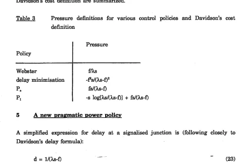
Webster's policy, nor delay minimisation are monotone with these cost assumptions.

[image:11.595.49.553.428.769.2]

In Table 3 all pressure definitions for the various policies in conjunction with Davidson's cost definition are summarized.

Table 3 Pressure definitions for various control policies and Davidson's cost definition

Policy

Pressure

Webster

delay minimisation

5 A new ragm ma tic power aolicy

which, of course, is too simple to be used in real-life, but which has the property that delays tend to infinity when flows approach capacity.

For this delay expression the three original policies can be expressed as follows:

Webster's Eq m s

=

Eq Uhs-0 for small flow f

Delmin Min Z f.d

=

Eq f ddlah

=

Eq fs/(hs-fy = Eq fiY2/(hs-0

and so, for appropriate values of k, all three policies can be expressed as

Tests described in Van Vuren et al. (1987) and Van Vuren et al. (1990) indicated that

a. Webster's policy performs well under low congestion: either mutual equilibrium has lower average travel time than Pds stable point.

b. Delay minimisation performs reasonable throughout a range of low to

medium congestion.

c. P,'s capacity maximising property is most useful when congestion is considerable.

Thus, if the power k in (27) is related to congestion, this policy can adapt itself to

mimic the behaviour of each of the three policies in the most appropriate range of conditions.

The value of k should be close to 1 if junction congestion is low, and close to 0 if congestion is high. An appropriate expression for k is:

with

an

upper limit of 1. Note that this power policy can only be readily applied

-.

of

(Is-f)

may change

if

flows are allowed to exceed capacity. Also, no monotonicity properties can be established for this policy:

it

is based on pragmatism and rather strong delay assumptions and should be tested thoroughly in a range of circumstances.

6 Tests on a

Bimale

network

The characteristics of the existing and newly developed policies will here be tested on a simple two-link network. This test network, as shown in Figure 0, consists of only four links, that make up two routes. The first route is fast, but with a limited capacity, e.g. through a town centre. The second route is longer, but wider, e.g. a bypass. Both routes meet a t the end of the town at a signalised junction.

The saturation flow a t the junction for the bypass = 4000 pculh, whilst the narrow town route has a lower saturation flow of 2000 pcu/h. The bypass is 150111 longer, so that at a free flow travel speed of 50 km/h its free flow travel time is 10.8 secs longer than that of the town route.

The following assumptions are further made:

-

cycle time = 60 see;

-

no intergreen times;

-

two stages, one for each road;

-

minimum and maximum green times of 0.5 sec and 59.5 sec respectively.

Firmre 0: Test network

First I will discuss test results with the BPR cost function, and three control policies

In these tests the iterative assignment control procedure is started from both edges of the feasible green time region, to investigate uniqueness of the resulting equilibrium, and the policies' abilities to move away from poor initial settings. In this two-link case the feasible region is straight-forward to determine, and the feasible boundary is determined by the minimum green time constraint. When applying the BPR cost function capacities are unlimited; with Webster's cost function, however, links are capacitated and the feasible green time region is directly dependent on total demand.

6.1 Tests with the BPR cost function

Figures 1, 2 and 3 show information about green time and flow distribution a t the mutual equilibrium plus associated excess travel times, related to total network demand and initial green times, using the BPR cost function (16). A comparison is given for the three policies and optimum NDP settings.

First note that, although monotonicity could not be established for either Po or Webster's policy, both give rise to single mutually consistent points.

The resemblance for this cost definition between the behaviour of Po and Delmin is striking. However, Po re-distributes traffic and green time to the wide route earlier, and resulting green times and flows are closer to the optimum. At low and high flow levels both policies give identical (and optimum) results, as expected.

With this polynomial delay function the Webster policy does not achieve any re- distribution to the wide route a t all, regardless of the total flow or the initial green time. This can be checked analytically as follows:

Signal control step (Webster's policy)

flhl~l =

f d b ,

User equilibrium assignment step

t

1

-

-

t,

(t

= 1

+

d)

11 >

4

(free flow travel time)

dl

<

d,

by shifting f

l,a[(fl-bf)h,s,lfl < &a[(f2+AD&s,In

Signal control step

(reduce

h,

to compensate for loss of flow; increase

&)

.-

Assignment step

(reduce fl to compensate for loss of green; increase f.J

lla[(f,-M-A1~/(~-~)sl]8 < &a[(f2+Af+A1f)/(&+Ah)sJn etc.

In words: flow and green time are persistently re-distributed to the narrow, shorter route until a feasible (minimum green time) boundary is met.

The performance consequence is represented in the average excess travel times in Figure 3. Up to a demand flow of approximately 1500 pcdh, some 75% of the narrow route's saturation flow, all 3 policies give rise to optimum mutual equilibria, whilst when approaching the wide route's saturation flow first Po and then Delmin again perform optimally. The comparative performance of Webster's policy deteriorates when the demand exceeds the narrow route's capacity, because no re- distribution of flow and green time to the wide route is achieved by this policy.

In the intermediate region Po performs about 20% better than Delmin, because of the early green timelflow re-distribution. An optimum, however, is not achieved

-

or even approximated

-

by application of any of the tested policies in that region.

6.2 Tests with Webster's cost function

Now capacities are finite; also the PI policy and Delmin are distinct. Both policies are also non-monotone with these cost assumptions. In addition to the three policies tested with the polynomial BPR cost functions four extra policies (PI,

,

,

P

P, and the power policy) will now be tested. Therefore, Figures 4, 5 and 6 are more complicated than the corresponding Figures 1 to 3. First note in Figure 4, which

depicts the green time distribution at equilibrium as a function of total demand, that because of the capacitated links an infeasible green time region exists.

Webster's policy and delay minimisation show virtually identical behaviour, ending up at one of the feasible boundaries; when demand exceeds the capacity of the narrow route (2000 pcuh) the lower limiting state will actually be unfeasible and therefore give rise to infinite delays and travel times. This limiting state ceases to exist at a total demand of approximately 2700 pcuh.

always give rise to feasible mutually consistent points.

Of the newly developed policies PI starts re-distributing flow and green time first.

As the policy is not monotone with Webster's cost function two equilibria emerge, a higher one and a lower one. Both follow closely the Webster and Delmin curves, but PI always gives rise to feasible solutions, because of its capacity-maximising properties. At a flow level of approximately 2400 pculh, when excess travel time starts rising rapidly, the lower limiting state merges with the upper solution and ceases to exist. -

P,, the monotone adaptation of P , shows a rather rigid behaviour, just like the other monotone policy, P,. Particularly striking is the rigid green time curve a t low flow levels for the P, policy, caused by the first term of its pressure definition: sC(1-h). As s, = 2s,, h,lb must be close to 2 to satisfy the equal pressure condition when the second term is small. Both policies give rise to unique and feasible solutions.

Of all new policies the power policy shows the most promising behaviour, closely following the optimum settings. A unique flowlgreen time pattern a t mutual equilibrium exists, which at low flow levels supports the narrow route. When the capacity of that route is approached, however, a complete swap-over to the wide route of both green time and flow takes place; note that this swap-over takes place later than for the optimum settings.

The final performance comparison is given by the excess travel times in Figure 6.

As observed before with sheared delay assumptions, the two conventional policies may end up in the very adverse situation in which only half the possible amount of t d c can be served. These curves go together with low excess travel times a t low demand levels, which steeply increase when the capacity of the narrow route is approached.

On the other hand, because of the two limiting states, if the starting point for the iterative process could be favourably chosen, these policies achieve near-optimum travel times at mutual equilibrium. The integrable policy

P,

follows the same pattern, but less extreme.

infeasible boundary of resulting green times. Of

Po

and

P

,

the first performs better and less rigidly, reacting to flows as well as saturation flows, giving rise to lower excess travel times in low and high congestion. Generally all monotone policies are rather insensitive to existing delays; for a considerable range of demand flows green time is split over both routes, even though all flow is assigned to just one of these. Resulting inefficiencies are the price we pay for theoretical uniqueness and existence of the mutually consistent points.

Overall, the power policy performs best, always ending up at a feasible point but, unlike the three capacity maximising policies, with green times optimally fitted to the flows. This gives rise to optimum behaviour, apart from the demand region between approximately 1860 and 1930 pc*, even there average excess travel time is lower than for most other policies.

7.1 Introduction

Performance of policies on simple networks is not necessary representative of their behaviour in reality. Tests on larger scale networks are needed for a better understanding and they will be presented next. They consist of:

(a) a network as used by Tan, Gershwin and Athans (1979) in their study of optimal signal control, here called the TGA network;

(b) the network of Weetwwd, a suburb of Leeds.

With these larger scale networks, simple calculations that sufficed for the two-link case have to make way for more sophisticated algorithms. For the equilibrium assignment the assignment subprogram of SATURN (Van Vliet, 1982) was used. Two adaptations to the program had to be made. Firstly the ability to control signals had to be introduced; secondly cost definitions had to be modified. For the polynomial BPR function this is a straightforward exercise and described in Appendix 4; the infeasibility of link flows above capacity with Webster's cost function, however, is incompatible with the requirements of the Frank-Wolfe algorithm that SATURN employs. An adaptation of Webster's cost function has been devised in order to comply with these requirements. This adaptation will be introduced in Section 7.2. Subsequently in Section 7.3, I will describe the green

-

-

assignment control procedure in the model. After this the results for both networks will be presented. I will discuss convergence of the algorithm, uniqueness of the resulting green times, and the quality of the mutually consistent points in terms of total network travel times a t those points.

7.2 An ada~tation of Webster's cost function

Webster's cost function has two properties that are incompatible with the Frank- Wolfe algorithm: -

(1) links are capacitated

(2) link costs approach infinity when the link flow nears capacity, and they are

undefined when the flow exceeds capacity.

The Frank-Wolfe algorithm, as a series of all-or-nothing assignments, needs link costs to be finite and defined throughout the whole flow region, also above capacity. The following adaptation of Webster's cost function is therefore developed.

Given a simulation period T (usually between 30 and 120 mins) the "kink" flow level is determined at which the derivative of Webster's cost function equals the deterministic queueing slope:

For flow levels above this value the continuation of Webster's curve is replaced by deterministic queueing, thus ensuring existence of

a

cost definition throughout the whole flow region, though at substantial cost close to or over capacity; and also ensuring a continuous first order derivative. Figure 7 shows Webster's cost function and its approximation; in the applications described next resulting flows that are

higher than the kink flow are considered to be infeasible. Appendix 5 presents the relevant mathematical expressions.

7.3 A preen time control aleorithm

Pressures, as defined by the control policy employed are analogous to costs:

link

pressures correspond to

link

costs and stage pressures, as a summation over constituent links, correspond

to

route costs. An equilibration of stage pressures can now be sought by swapping green time from less pressurised to more pressurised stages (like an equilibration of route costs is sought by swapping flow h m higher cost routes to cheaper ones),

As

the number of stages at a junction is limited (and known in advance) an algorithm that needs stage enumeration can easily be applied. The algorithm employed here is based on that described by Dafermos and Sparrow (1969) and it works as follows.

For each junction:

(1) determine link pressures (based on flow and green time);

(2) determine stage pressures (by summing over constituent links as determined by the stage matrix);

(3) determine minimum and maximum pressurised stages;

(4) determine an optimum swap of green time from the minimum to maximum pressurised stage, subject to feasibility constraints;

(5) unless convergence is achieved, go to step 1.

This algorithm will determine a set of green splits consistent with a fixed set of flows, as in (6). A number of observations with respect to this algorithm must be made:

-

for most control policies a stage pressure is defined in step 2. by a summation over constituting link pressures; for Webster's control policy, however, a stage pressure is determined by the maximum of constituent link pressures;

-

_{determination of an optimum amount of green time to be swapped from the} minimum to the maximum pressurised stage is carried out by

a

golden section search;

-

convergence can be monitored via the step size determined for the optimum green swap.

7.4 Im~lementation asoeds of the iterative assienment control orocedure

In Smith and Van Vuren (1990) a variant of the iterative assignment control procedure is introduced, which might reduce its computational burden. Instead of carrying out the assignment step till convergence, we might suffice with a single iteration in the assignment, consisting of a direction search via an all-or-nothing load and a subsequent optimum step size search. Even though the assignment objective function would not be minimised in each step, it would definitely be decreased, and the large number of assignment-control iterations should ensure that a mutual equilibrium will be reached in the long run, independent of the actual algorithm employed.

Two implementations have been tested, namely the full implementation that converges each assignment sub-step, and the streamlined version that allows only one new route per assignment. The two implementations were tested on the Weetwood network, with a maximum number of assignment-control iterations of 200,

the observed OD-matrix and the delay minimising control policy. Resulting computation times with both polynomial delay assumptions and Webster's cost funcion are shown in Table 4

Table 4 Computation times for two implementations of the iterative assignment control procedure and two different cost functions. Weetwood, 1.0 x OD, 200 iterations.

full implementation streamlined version polynomial costs (BPR) 28.21 sec 26.41 sec

Webster's costs 72.92 sec 63.60 sec

First note in Table 4 the difference in computation times between polynomial cost assumptions and Webster's costs; compared with these the computational savings of the streamlined algorithm are limited. This is related to the convergence performance of the iterative assignment control procedure, which is not unlike that of the Frank-Wolfe algorithm. As a rule only in the first few steps of the iterative assignment control procedure a relatively large number of iterations is reguired to

.<

green time changes and consequent flow changes are so small that single route changes suffice for convergence, governed by the size of the step length h and the uncertainty in the objective function. This also means that savings in computation time by the streamlined algorithm will be of an absolute, rather than relative nature, as they are achieved in the first few iterations only. The streamlined algorithm has been implemented and used in the test runs described next.

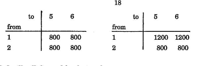
8 Results for the

TGA

network

The network introduced by Tan et al. (1982) consists of 8 uni-directional links, 6 nodes and 4 OD-pairs. Although still small in size, the network presents a much more realistic situation than the simple network used before; four OD pairs exist and each of the OD pairs has 2 or 3 routes available that do not necessarily pass the signal-controlled junction.

The network is shown in Figure 9; node 3 is signal-controlled. All links have saturation flows of 1500 pcuh, apart from the link between nodes 4 and 5 which has a capacity of 3000 pculh. Link lengths are given in the Figure and the h e flow speed is assumed

to

be 40

k d .

Some differences with the approach of Tan et

al.

must be noted:

(1) Tan et a1 apply the BPR cost function to all links in the network; in addition they apply Webster's cost definition to those links that are signal controlled.

I have chosen to apply Webster's cost definition only to links a t signalised junctions, whereas links at non-signalised junctions have their cost calculated according to the sheared delay curve; in effect this will make non-signalised junctions generally less attractive than in the network used by Tan et

al.

(2) Cycle times are 60s and 75s respectively for Tan et a1 and my TGA network. These differences will explain why the results &om the two studies differ, even though the conclusions that are drawn h m them are very similar.

which I will call demand levels 1 and 2.

to from

1 2

I will reproduce these tests for the two cost functions and control policies I described before; and like Tan et al. I will compare the performance of each of these policies with the user optimum.

(NB

As this network contains only one signal-controlled node with 2 stages the user optimum can be found via a simple one directional search method). In addition I will investigate the following demand patterns:

and I will call these demand levels 3 and 4.

5 6 to

from

800 800 1

800 800 2

8.1 Results with the

BPR

cost hnction

5 6

1200 1200 800 800

Results for iterative assignment control with the polynomial

BPR

cost dehition and the three relevant control policies are given in Table 5.

Table 5: _{Resulting green times and total travel times for} three policies and varying demand levels, compared with optimum settings; polynomial cost definition

demand demand demand demand

level 1 level 2 level 3 level 4

T T T G T T T G T T T G T T T G

Webster 773 0.16 1057 0.26 357 0.35 1075 0.03

Delmin 776 0.20 1059 0.29 357 0.35 1075 0.03

Po

777 0.21 1060 0.30 357 0.36 1075 0.03

optimum 771 0.11 1057 0.25 357 0.35 1075 0.03

[image:22.595.105.468.65.179.2]

Resulting green times turn out not to depend on the initial split and therefore only a single green split and associated total travel time is shown for each policy in Tables 5 to 10. As in the two-link case the behaviour of the three policies is very similar and also very close to the optimum. Of the three policies Webster's gives rise

to

the most uneven split, generally favouring the in-link from node 2. This can be explained by the observation that the free flow

link

cost of the alternative route from this node (2-5) is much higher than the route via the signalised junction, certainly compared with the route alternatives that exist for t&c originating a t node 1. Whilst for the relations 2-5 and 2-6 this difference is 2.5 miles (360 sec) and 3.5 miles (504 sec), for the relation 1-6 the difference is only 0.5 miles (72 see). Therefore, with the polynomial cost definition traffic will re-route quicker to the alternative on relations from 1 and Webster's policy (to equalise degrees of saturation) will favour the larger traffic stream from node 2. The extreme behaviour of Webster's policy in the two-link case is not reproduced here, however.

The attempts of

Po

to reroute t d c from 2 away from the signalised junction fail because of the large extra length of the alternative and the comparatively shallow f o m of the BPR cost fundion.

This also results in actual oversaturation at the signalised junction for all but the lowest demand levels, irrespective of the control policy used.

This behaviour is further illustrated by Table 6 which shows resulting green splits and total travel times for demand level 2 and a shortened bypass from node 2 to node 5 of 6.25 miles instead of 8 miles. Now Po does manage to redistribute traffic away from the signalised junction, resulting in an improved behaviour over Webster's policy and delay minimisation. Again, however, the signal-controlled junction is oversaturated, but to a lesser extent, due to the use of a polynomial cost

Table 6: Resulting green times and total travel times for three policies and demand level 2; shortened bypass and polynomial cost definition

Webster 1030 0.30

Delmin 1024 0.35

Po 1023 0.36

TTI' = total network travel time in veh h r h

G = green split for link 1-3

8.2 Results with Webster's cost function

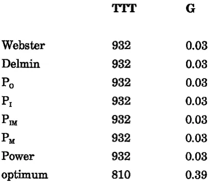
With Websteis cost hnction I investigate the behaviour of 7 policies; the base case is demand level 1 with 800 pcdh on each OD-relation. Table 7 shows the results; note that these are again unique, independent of the initial green split (even though monotonicity could not be established for five policies).

Table 7: Resulting green times and total travel times for seven policies and Webster's cost function, demand level 1

Webster Delmin

Po

PI

p, PM Power optimum

TTT

= total network travel time in veh hr/hr

[image:24.595.79.285.500.681.2]

The Table c o n b s the findings of Tan et al., that iterative assignment control does not find a user optimum for this configuration. Even more, this is irrespective of the policy employed. A full allocation of green time to the in-link from 2 takes place, forcing most traffic from origin 1 to take the alternative route that avoids the signalised junction. Application of Webster's cost function ensures, however, that all link flows are within capacity, mainly by routing nearly all flow from origin 1 to link 1-4.

When the demand level for relations from, origin 1 is increased to 1200, however, my findings are rather different from Tan et al. (demand level 2; Table 8). Again the iterative assignment control procedure cannot find the optimum settings according to network design; with these demands, however, the capacity maximising policies perform better. These policies give more green to the in-link from 1, thus forcing traffic from 2 to re-assign to the bypass; the signal-controlled junction is still undersaturated.

Table 8: Resulting green times and total travel times for seven policies and Webster's cost function, demand level 2

Webster Delmin Po pz pm PM Power optimum

?TT = total network travel time in veh h r h r

G = green split for link 1-3

Based on these results Tan et al. reject the iterative assignment control procedure. However, not only do my results show that the use of different control policies can improve its performance, but in addition

it

is rather limited to base such judgements

[image:25.595.83.291.428.609.2]

Therefore I investigate two more demand levels: a low demand level with only 400 pcdh on each OD relation (demand level 3) and a demand level with increased flows on all relations from origin 2 (demand level 4). Table 9 shows the results for demand level 3.

Table 9: Resulting green times and total travel times for seven policies and Websteis cost function, demand level 3

Webster Delmin

Po PI PM p, Power optimum

TTT = total network travel time in veh hr/hr

G = green split for

link

1-3

For this demand level all policies perform well, particularly the non-monotone policies that follow and accept flow levels as they are, without attempting flow re- distribution. Again, none of the policies finds exactly the user optimum, but differences are now very small indeed.

[image:26.595.72.543.130.445.2]

Table 10: Resulting green times and total travel times for seven policies and Webster's cost function, demand level 4

Webster Delmin Po PI p* PM Power optimum

TTT = total network travel time in veh hr/hr G = green split for link 1-3

Again all policies end up at a mutually consistent point at the minimum green time boundary for link 1-3, caused by the weight of the OD-flows from origin 2. As

before, this is not the user optimum (differences in total travel times exceed lo%), but link flows remain within capacity.

8.3 Conclusions TGA network

Summarising, although the iterative assignment control procedure for this network and the demand levels tested never finds optimum signal splits, it does not perform as bad as Tan et al. claim. I do not claim that the procedure is an actual heuristic for the network design problem; it is

a

practical tool for use in large scale networks, allowing a realistic network description and complex cost functions. The procedure in this case gives rise to sensible signal splits and its extreme behaviour in two of the cases is strongly determined by the network layout. It would be just as easy to

construct a network on which the iterative assignment control procedure performs well in conjunction with d l or particular policies, and in my view final conclusions should be based on more tests with realistic networks.

[image:27.595.83.294.133.319.2]

matter to the practitioner, is the influence of the control policy employed and the cost assumptions on resulting green splits and accompanying travel times.

Of the control policies investigated the capacity maximising policies probably perform best; the performance, however, is strongly influenced by the quality of the available route alternatives. Of these four policies (Po, P,, P, and P,), Po performs best and has the added advantage that it can be applied independently of the cost function employed. The power policy performs promisingly, but needs testing on a larger scale network. Finally, Webster's policy performs most extremely, particularly under Webster's cost definition.

The cost function employed influences the results of the iterative assignment control procedure in two important ways:

(1) It iniluences the performance of each of the policies, with respect to the quality of the mutual equilibrium reached.

(2) It influences resulting green times, not only for each of the policies, but also the optimum settings.

A

comparison of green times in Table 5 and those in Tables 6 to 10 will back this up. The question is, of course, which green splits are optimal in reality.

9 Results for the Weetwood network

The Weetwood network is of a much larger size than any of the previous networks tested. It consists of 70 zones, 105 nodes and 442 directional links. Of the nodes, 17 are signal controlled with 42 stages in total. The network is depicted in Figure 10; the modelled situation is the AM Peak with strong North-South flows.

As before, this network is tested with:

(a) different cost assumptions (b) different demand levels

(c) different control policies

(d)

different initial green time splits.

9.1 Results with the BPR cost hnction

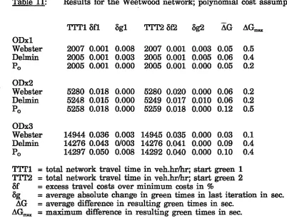
With the polynomial cost function three demand levels have been investigated. The base case is the observed trip matrix, giving rise to an average network speed of 35- 40 km/h (dependent on initial green time splits). To allow for a considerable increase in congestion, and because of the shallow form of the cost function, the two other demand levels investigated are for a doubled and trebled OD-matrix, giving rise to speeds of approximately 20 k d h and 10 k m h respectively. Results for these tests are shown in Table 11; as before, three control policies (Webster, Delmin and Po are tested in interaction with user equilibrium assignment.

The iterative assignment control procedure has been started h m two different initial green splits. The Table shows resulting total network travel times a t the two mutually consistent points found and the average and maximum differences between resulting green times a t those points; cycle time is 100s.

Table 11: Results for the Weetwood network; polynomial cost assumptions

ODxl

Webster 2007 0.001 0.008 2007 0.001 0.003 0.05 0.5 Delmin 2005 0.001 0.003 2005 0.001 0.005 0.06 0.4 Po 2005 0.001 0.000 2005 0.001 0.000 0.05 0.2

ODx2

Webster 5280 0.018 0.000 5280 0.020 0.000 0.06 0.2 Delmin 5248 0.015 0.000 5249 0.017 0.010 0.06 0.2 Po 5258 0.018 0.000 5259 0.018 0.000 0.12 0.5

ODx3

Webster 14944 0.036 0.003 14945 0.035 0.000 0.03 0.1 Delmin 14276 0.043 01003 14276 0.041 0.000 0.09 0.4 Po 14297 0.050 0.008 14292 0.040 0.000 0.10 0.4

TIT1 = total network travel time in veh.hr/hr; start green 1 TIT2 = total network travel time in veh.hr/hr; start green 2 Sf = excess travel costs over minimum costs in %

Sg = average absolute change in green times in last iteration in sec. AG = average difference in resulting green times in sec.

AG,, = maximum difference in resulting green times in sec.

[image:29.595.66.469.397.710.2]

total network travel costs with current flow pattern total networks costs via minimum routes

and this is a measure how far we are from an equilibrium, in which case the value of 6 = 0. They show how well the procedure has converged, with excess travel costs never more than 0.05% and an absolute average change in green times in the final control iteration of less than 0.01 sec.

As in previous tests with this cost assumption, the results of all three policies in the iterative assignment control procedure are very similar. The maximum difference in travel times between delay minimisation and Po is limited to tenths of a percent, and the maximum difference with Webster's policy is less than 5%. Also the resulting green split patterns are virtually independent of the initial splits (even though monotonicity could not be established for either Po or Webster's policy). The small differences in green splits resulting from each of the starting points are most likely due to computational inaccuracies.

A closer look at the resulting green splits also reveals that the final splits do not necessarily depend very much on the control policy employed, as Table 12 shows. Although average differences in resulting green splits may run up to some 8 sec between Webster's policy and the two other policies and maximum differences up to

27 sec, particularly striking is the similarity of final green splits for Delmin and

P,,.

Differences in resulting network travel times are always less than 0.1% and the maximum difference in final green times is 2.0 sec in the 1.0 case and 6.4 sec in the

3.0 case (average differences are 0.7 sec and 1.6 sec respectively), almost the same order of magnitude as the differences resulting h m different start greens.

Table 12: Differences in final green times between the three policies; start green 1

ODxl

- ODx3 -

AG A

G

,

,

AG AG-

Webster-Delmin 3.3 9.4 6.2 21.3

Webster-Po 3.9 10.9 7.6 27.1

Delmin-Po 0.7 2.0 1.6 6.4

-

AG

= average difference in resulting green times in sec.

9.2 Results with Webster's cost function

As

links are capacitated with Webster's cost function congestion builds up much more rapidly than with polynomial delay assumptions. This is demonstrated by the steeper rising total network travel times in Table 13; in fact no feasible flowlgreen time pattern (where feasibility is defined as: "with all signal-controlled links below artificial capacity as defined by the "kink" flow in paragraph 7.2") could be found by any of the policies for demand levels higher than 1.2 x observed demand.

N.B. In effect, this is not really a feasibility problem. An appropriately large choice of simulation time T would:

(a) shiR the kink flow to the right, as the slope of the over-capacity delays increases;

(b) ensure sufficiently high delays near capacity to re-distribute tr&c away @om signalized junctions.

Extremely large T s and steep slopes in the cost functions, however, introduce instabilities in both assignment and signal control, and therefore a limited value of 9999 min. was applied to determine the over-capacity slopes of delays at signalized junctions, and 30 min. at all other junctions.

Comparing total network travel times, we can first observe the rather good behaviour of Webster's policy at lower congestion (though never better than Delmin) and the rather poor behaviour when network capacity is approached (OD x 1.2); then total travel times are up to 19% higher than for Delmin. Delay minimisation perf01111s very well and consistently; Po is as consistent, though resulting travel times are 2-3% higher than those for Delmin. PI generally performs slightly better than Delmin.

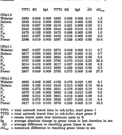
Table 13: Results for Weetwood network; Webster's cost assumptions

TTTl Sfl Sgl

ODxl.0

Webster 2392 0.056 0.005

Delmin 2349 0.013 0.000

Po 2416 0.057 0.008

PI 2343 0.022 0.008

pm 2475 0.105 0.005

PM 2421 0.037 0.000

Power 2366 0.019 0.003

0Dxl.l

Webster 2867 0.027 0.010 2874 0.046 0.005 0.11 0.7

Delmin 2817 0.058 0.000 2819 0.057 0.003 0.12 0.7

Po 2885 0.026 0.005 2884 0.030 0.003 0.05 0.2

PI 2787 0.036 0.000 2795 0.070 0.010 2.23 23.4

PIN 3014 0.416 0.005 3017 0.037 0.008 0.05 0.2

PM 2894 0.056 0.013 2893 0.029 0.023 0.05 0.2

Power 2807 0.049 0.008 2765 0.073 0.000 3.48 27.3

ODx1.2

Webster 3853 2.346 0.035 4156 2.479 0.010 1.62 9.1

Delmin 3485 0.199 0.013 3443 0.310 0.008 2.15 16.4

Po 3520 0.372 0.000 3521 0.376 0.023 0.10 0.4

PI 3370 0.125 0.003 3360 0.106 0.013 0.09 0.5

PIN 3869 0.014 0.000 3901 0.018 0.008 0.09 0.3

PM 3559 0.072 0.000 3558 0.057 0.000 0.10 0.4

Power 3417 0.110 0.010 3376 0.202 0.005 2.10 16.3

TTTl = total network travel time in veh.hrb, start green 1

TTT2 = total network travel time in veh.hr/hr; start green 2

6f = excess travel costs over minimum costs in %

6g = average absolute change in green times in last iteration in sec. AG = average difference in resulting green times in sec.

AGm, = maximum difference in resulting green times in sec.

Again the convergence of the iterative assignment control procedure has been monitored via excess travel costs 6f and the absolute average change in green times in the final iteration Sg. It is important here to note that no stop criterion was applied to the procedure, apart from the maximum number of 500 iterations.

Apart from Webster's policy in the highly congested case the convergence of the assignment process is excellent, indicated by final excess travel costs for all other

policies of less than 0.4%. This level of convergence is backed up by the average absolute final change in green times, which in this case is always less than 0.03 sec. Note how the convergence is negatively influenced by an increase in congestion.

An interesting picture is painted by the stability of the seven policies, expxessed in

-

[image:32.595.80.493.98.557.2]

increase in congestion; this is much more so than with polynomial cost assumptions (Table 11). Least stable in resulting green splits is the power policy, with an average difference of up to 3.5 sec and a maximum difference of up to 27.3 sec in green splits resulting from different starting points, even though this does not express itself in widely differing total travel times. The same argument, but to a lesser extent, is valid for P;s behaviour and delay minimisation; Webster shows considerable differences in total travel times, as well as in resulting green times when congestion is high. Po and the two monotone policies P, and P, are most stable; particularly striking is the similarity in performance and stability between

Po

and

P

,

.

A vital element of the power policy, the power k, deserves more attention here. I

am particularly interested in:

(a) development of k-values during the iterative process and (b) stability of its final values.

Table 14: Final values for power k dependent on initial green splits; Weetwwd network; OD x 1.1

value k value k

node start green 1 start green 2

[image:33.595.82.552.375.690.2]

of the iterative procedure. Their final value, however, depends on the initial green time settings as Table 14 shows more clearly, as initial timing influences the final flow and green time pattern.

9.3 A more dvnamic examale

Up to now all numeric examples had a fured level of demand, for which signals were adjusted according to a chosen control policy. The iterative assignment control procedure can, however, be used to represent:

(a) regular updating of fixed time signal plans after traf6c has re-adjusted to changed conditions

(b) performance of vehicle-actuated control over time.

In both cases drivers need time to experience changing conditions and to adjust their route choice accordingly. The assumption of fixed demand is rather restricted, given the current tmffk growth of some 2.5% per year. Therefore, in this example, a dynamic adjustment of travel demand is allowed after each signal control step, to represent traffic growth. This traffic growth is set to 0.05% per step; in case (a) this would represent an update of the signal plan every week (maybe rather unrealistically); in case (b) this would represent a learning period for drivers of approximately 1 week.

The iterative assignment control procedure was started for the Weetwood network with a demand level of 1.1 x observed

OD

flows and again the two different initial green splits. Table 15 shows per policy resulting demand levels a t which the flowlgreen time pattern becomes infeasible; Webster's delay formula was employed.

Table 15: Maximum demand levels that give rise to feasible flowlgreen time combinations; Weetwood network; Webster's cost function

control policy Webster Delmin Po PI

p,

PM Power

maximum maximum

Of all control policies Webster's definitely performs worst: the maximum demand level that still gives rise to feasible flowlgreen time combinations is only slightly more than 1.2 x observed demand and for one set of start green splits the policy actually never settles down to a feasible solution. The capacity maximising policies (Po, P,, P, and P,) all perform better than delay minimisation, in that they indeed allow a higher demand level to be processed by the network, but there is a clear influence of initial settings. Also all capacity maximising policies should theoretically give rise to equal maximum demand levels, as in the two-link example. The adaptation of Webster's cost function will play a role here. Particularly impressive in their performance are PI and P,, but it is the power policy that is really surprising. It outperforms all other policies, even the capacity maximising ones and gives rise

to

highest feasible demand levels.

Another view on these results is given by Figure 13, which depicts total network travel time per policy against the increasing demand level, for the case with start greens 1.

With Webster's policy the iterative assignment control procedure does not settle down to a feasible solution until a demand level of approximately 1.17 x observed OD flows and at a level just above 1.20 x observed demand a t least one of the signal controlled link flows becomes infeasible. During this short feasible region network travel times are higher than for any other policy.

The poor behaviour of the P, policy, that already emerged from Table 13, is again illustrated. Delay minimisation gives rise to very advantageous settings at lower demand but travel times increase rapidly and infeasibility occurs a t a demand of 1.23 x observed OD-flows.

It was observed before that Po and P, show a very similar behaviour, which is confirmed by the graph; P, maintains feasibility longer than P,,. Finally, PI and the power policy perform very alike, apart from the highest feasible demand levels where the power policy gives rise to lower total travel times; in addition this policy maintains feasibility longest.

9.4 Conclusions for the Weetwood network

In the first place the streamlined version of the iterative assignment control procedure converges extremely well in virtually all cases, as indicated by the values of Sf and Sg.

Secondly none of the policies shows as extreme a behaviour as in the two-link example, or even the TGA network. A feasible boundary of the flowlgreen time space is seldom reached, so that delay minimisation in general shows the best behaviour of all policies, despite potential theoretical problems.

The monotone policies are most stable, as expected, but 2-13% less efficient than Delmin. The need for capacity-maximising properties is not apparent in this network; of all four capacity-maximising policies

Po

is preferred. It generally outperforms the other policies and is applicable with a l l cost functions.

Of the remaining policies Webster expresses the most unstable behaviour, particularly at high congestion. The pragmatic power policy's performance is very promising in terms of total network travel times, but rather unstable in resulting green splits; it seldom improves on Delmin.

The cost function employed has

at

least as important an effect on results as the choice of control policy. With polynomial cost assumptions all three policies tested behave in a very similar way, giving rise to virtually identical network travel times. When employing Webster's cost function the network capacity is limited and the influence of the control policy used on network performance and stability of green splits is much more pronounced.

Table 16:

Webster Delmin

Po

Differences in results with Webster's and polynomial cost assumptions; Weetwood network, OD x 1.0, start green 1

-

TTT-BPR ?rr'-WEB AG AG-

= total network travel time in veh.hr/hr; BPR cost function

= total network travel time in veh.hr/hr; Webster's cost function

= average difference in resulting green times in sec. = maximum difference in resulting green times in sec.

Because of the congestion characteristics of the two cost functions only the observed case (OD x 1.0) can be compared. Not surprisingly, total network travel times are

some 20% higher with Webster's cost definition than under the BPR assumptions, although in fact the shape of the polynomial delay function should be calibrated via the parameters a and

13.

More importantly, and less dependent on such a calibration, the resulting green times are totally dissimilar under the two cost definitions, as average and maximum green time differences illustrate. This indicates the limited value of modelled green splits for real-life use, unless a very realistic cost definition is applied. This will be the subject of the next Chapter.

10.

REFERENCES

Dafermos SC and Sparrow FT (1969) "The traffic assignment problem for a general network" J Res Nat Bureau of Standards, Vol 73B, Nc2, pp 91-118

Heydecker BG (1983) "Some consequences of detailed junction modelling in road traffic assignment" Transportation Science, Vol 17, Ne3, pp 263-281

Poorzahedy H and Turnquist MA (1982) "Approximate algorithms for the discrete network design problem" Transportation Research, Vol 16B, Ngl, pp 45-55

[image:37.595.79.509.93.327.2]

Smith MJ (1981) "Properties of a traffic control policy which ensure the existence of a traf3ic equilibrium consistent with the policy" Transportation Research, Vol 15B, N26, pp 453-462

Smith MJ and Van Vuren T (1990) "Traf3ic equilibrium with responsive t r f i c control" Submitted to Transportation Science

Smith MJ, Van Vuren

T,

Heydecker BG and Van Vliet D (1987) "The interaction between signal control policies and route choice" In Gartner NH and Wilson WHM (eds) "Proceedings of the 10th International Symposium on Transportation and Traffic Theory", Cambridge, Massachusetts, Elsevier, New York, pp 319-338

Tan H, Gershwin S and Athans M (1979) "Hybrid optimization in urban traf3ic networks" Final Report, US-DOT-TSC-RSPA-79-7

Van Vliet I3 (1982) "SATURN

-

a modern assignment model" Trafic Engineering and Control, Vol 23, pp 578-581

Van Vuren T, Smith MJ and Van Vliet D (1987) "The interaction between signal setting optimization and re-assignment: background and preliminary results"

Transportation Research Record 1142, pp 16-21

35 _-

_.

Fimre 1 Green time at mutual equilibrium for four policies; 2-link test network;

36 _{- .}

[image:43.595.66.507.140.726.2]

Figure 5 _{Flows on bypass at mutual equilibrium for seven policies; 2-link test}

Fieure 6 _{Excess travel time at mutual equilibrium for seven policies; 2-link test}

[image:45.595.79.534.138.765.2]

41

43

44

[image:49.595.57.556.83.794.2]

Fipure.12 Development of power k in the iterative assignment control procedure;

47 _{- .}

48

APPENDIX 1: Monotonicitv with BPR delav function

For a solution to the combined assignment signal control problem to exist and to be unique the vector (t,-p) should be the gradient of a convex function V.

(t,-p) is the gradient of function V if

av/af =

t

and av/ah = -p

If V is smooth, and thus

we can express p as follows:

V is convex iff the gradient (t,-p) is monotone so that the Jacobian of this vector is positive semi-definite. The Jacobian is

Even if (t,-p) is not a gradient monotonicity of (t,-p) is a desirable property, because then a convex set of equilibria is guaranteed to exist; which may be unique in that

it may consist of a single point (Smith, 1982). (t,-p) is monotone iff

IImll

2 0 ; (Smith, 1985).

2

This is clearly a slightly weaker condition than that mentioned above; here the symmetrized Jacobian must be positive semi-definite.

t =

at.

P/hBsP

v

=

j

t(x)dx =

at.

u(p+i)

P'~ILPSP

0

so that PI is monotone

Delmin: p = f at/ah

so (t,-p) is monotone for delay minimisation

Webster

51

- .

APPENDIX

2: Monotonicity with Webster's cost definition

Apart from the factor 112, this expression can be divided into 2 terms

First term (t1)

PI = -3VIah = -2sC(1-h)log(l-US) for policy PI

llM1l

= C(1-h)'I(l

-

Us)'

.

(-2C log(1

-

Us)

-

4C) 2

Thus, the Jacobian is not positive semi-definite and the fmt term of policy PI is not monotone. To ensure montonocity a correction term must be introduced in policy

P Properties of this correction term include:

-

I$I is function of h only

-

_aI$I/ah = 4sC (as -2C log(1

-

Us's) 2 0)

at,/af, atl/ah, ap,/af as before ap,/ax = ~ S C ~O~(I-US'S)

-

~ S C

and thus the first term of P, is monotone

Second term (t,)

Pa = -dV/ah = d(hs-f)

-

m 2 s

-

llh for policy PI

= l/h2 [ ( 1 - 2 f i ) / ( h ~ - D ~ - l/h2s21

= 1h2 {(hs-f)Y[(hs-f)2h2s21

-

P~h2sYhs-f)21

-

llh2~2)

Correction term @ must be function of h only, so no @ emerges naturally from the above. However, if we try @ = ILL (to compensate the integration constant):

and so the second term of P, is monotone too

PM Policv

This policy is characterised by the following pressure definition:

This pressure consists of two elements, each one associated with part of Webster's cost function. The term sC(1-h) is associated with Webster's first term; note the similarity with policy P;s first term. The term sl(hs-f) resembles the second

term

of PI and is associated with the second part of Webster's cost function. The resulting vector (t,-p) is not a gradient for this pressure, but monotonicity can be established.

First term

so first term of P, is monotone

Second term

55

APPENDIX 3: Monotonicity with Davidson's cost function

Here we concentrate on delay term (hs/(hs-f)

-

1)

= -hs log (As-f)

-

f

+

hs lodhs)

p = -aVAh = hs2/(hs-f)

+

s log(b-f)

-

s 10g(hs)

-

s

= -s lodhsl(hs-f)]

+

fsl(hs-f) for policy PI

Thus policy PI is monotone with Davidson's cost function.

Therefore, delay minimisation with Davidson's cost assumptions is not monotone.

And thus the P, policy is not monotone either.

Webster

57