Adaptive Gain Control for a Two Axis, H Frame Type, Positioning System

Article

Adaptive Gain Control for a Two-Axis, H-Frame-Type,

Positioning System

Gridsada Phanomchoeng

*

and Ratchatin Chancharoen

Department of Mechanical Engineering, Faculty of Engineering, Chulalongkorn University, Bangkok 10330, Thailand

*E-mail: [email protected]

Abstract. XY gantry systems play an important role in many applications in diverse industries, where they are used to position a part or tool along the xy plane within the working area of the system. The increased demand for enhanced performance and low cost of XY gantry systems has driven research to develop alternative structural designs and improve their capabilities. A two-axis, parallel H-frame XY positioning system (H-Bot) is of increasing interest as a candidate for development due to its low number of moving parts, lightweight, low cost and speed of the system. However, the system has an uncertainty of cart or end-effector position when moving at high speed because of the friction and flexibility of the elastic timing belt. The H-bot developed here using an adaptive gain control showed a good repeatability and improved accuracy, reducing the root mean square error between the desired and the actual trajectory of 32.7% and 53.2% on the x-axis and y-axis, respectively, for drawing a 80 mm diameter circle in 36 seconds.

Keywords: H-bot, H-frame, two-axis parallel positioning system, recursive least squares (RLS), linear least squares, adaptive control.

ENGINEERING JOURNAL Volume 21 Issue 3 Received 5 August 2016

Accepted 27 October 2016 Published 15 June 2017

1.

Introduction

XY gantry systems play an important role in many applications in diverse industries, where they are used to position a part or tool along the xy plane within the working area of the system. Many varied types of applications, such as pick-and-place, dispensing, cutting, welding or automation, require the system. Currently, most XY gantries consist of linear stages, ball/lead screws or timing belts. By stacking linear stages on top of each other and perpendicularly aligning them, an XY gantry system is made [1]. The XY gantry systems with this configuration are widely used in industry because of their reliability, resolution, repeatability and accuracy [2].

It is clear that the performance of this type of gantry system is outstanding [3-6]. However, systems with this configuration still have some disadvantages. Their size is large and they require a high power motor because one linear stage always needs to carry the other stages. Thus, the speed of this system is low [1]. Moreover, additional components are required, such as an energy chain (E-chain) system for the wiring system of the linear stage which is installed on the others. Also, their cost is quite high because of their components and the structural design of their system.

The increasing demand for enhanced performance and low cost of the XY gantry systems has driven research to develop alternative structural designs and improve their capabilities [7]. A two-axis, parallel, H-frame XY positioning gantry system (H-Bot) is one example that has become of increasing interest to develop its performance [1, 7-10] due to its lower number of moving parts, lightweight, low cost and high speed.

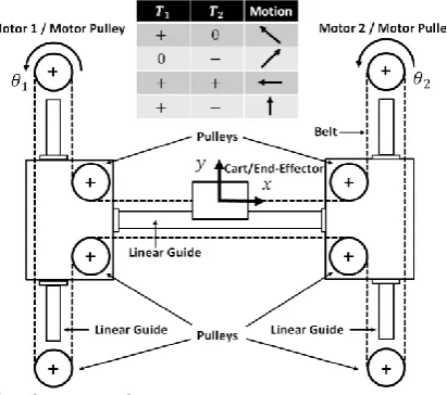
The configuration of the H-Bot is shown in Fig. 1. The system consists of two parallel linear guides and one linear guide perpendicular to them to from an H-shaped frame. Then, two motors are installed on the H-shaped frame and connected by a single circumferential timing belt. With this configuration, the motors are stationary and the guides are in the same plane. Only a cart or end-effector with a small mass is moved, and so the system is potentially capable of fast acceleration and has a low inertia [1, 5].

Fig. 1. Layout of the H-Bot/H-frame configuration.

Even though the configuration of the H-frame XY positioning system is suitable to handle industrial work, the system still has disadvantages. The flexibility of the elastic timing belt causes a stretching problem, while the system has a nonlinear friction increasing with speed, which causes an uncertainty in the cart or end-effector location when operated at higher speeds [1, 8]. Therefore, it is necessary to develop algorithms and techniques to improve the performance of the H-frame XY positioning system.

To improve the accuracy of the position of the H-frame XY positioning system, a closed-loop control with proportional integral derivative (PID) controller was applied [1, 9], while a nonlinear PID with four DOFs model was developed to control the system [8]. Overall, these controllers seemed to improve the accuracy of the H-bot.

Although other researchers have tried to solve the elastic drive and friction problems, these were not applied to the H-frame XY positioning system. For example, elimination the elastic transmission effect using a feed-forward compensator and fuzzy-logic base [11, 12], improving the accuracy of the position by compensating the friction with an adaptive control [13], and designing an estimator to estimate the friction of the system and compensate for it [14, 15].

The application of diverse techniques, such as using high order dynamic model or applying nonlinear control techniques, have been applied to improve the performance of the H-frame XY positioning system with some success [1, 7-10], but none of these have applied adaptive control gain on the H-frame XY positioning system. Thus, this study investigated the use of adaptive control gain to improve the accuracy of the cart or end-effector of the H-bot system.

The systematic design of the control system was composed of the three steps of the (i) kinematic model of the H-frame XY positioning system, (ii) low level PID control and (iii) high level adaptive gain control. This report is accordingly organized as follows. Section 2 describes the design and implementation of the H-frame XY positioning system, as well as the experimental setup and kinematic model. Section 3 investigates the accuracy of the system with a simple PID controller. Section 4 presents the constant gain control and adaptive gain control along with the results of their evaluation in use, and finally Section 5 presents the conclusions of this study.

2.

The H-Frame XY Positioning System

2.1. The Setup of the System

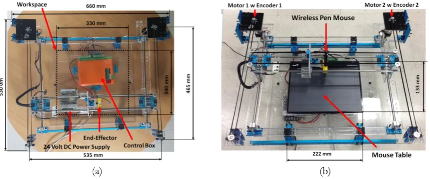
The developed H-frame XY positioning system is shown in Fig. 2. It consists of two parallel linear guides and one linear guide perpendicular to the parallel linear guides to form a H-shaped frame. A pulley was installed on each end of the parallel linear guides, while there were two pulleys on each end of the perpendicular linear guide. The diameter of all the pulleys was 12 mm and a timing belt was guided around these eight pulleys. Two 24-V DC motors (Escap 28DT2R 12 222 E 103) were installed at the end of the parallel linear guides and were equipped with optical encoders (HEDS-5500 C11) with a resolution of 100 pulses per revolution. The overall size of the system was 530 x 660 mm with a workspace of 340 x 330 mm.

(a) (b)

Fig. 2. Components of the (a) system and (b) sensor (wireless pen mouse and mouse table).

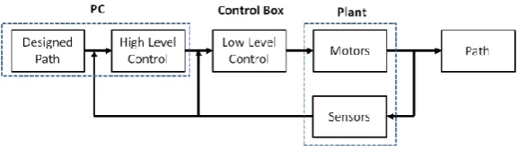
on the controller box and the high level control was developed on the PC. The architecture of the system control is shown in Fig. 3.

Fig. 3. Control architecture of the system.

In order to improve the accuracy of the system, a wireless pen mouse and mouse table (G-Pen F509 by Genius) were installed on the system, as shown in Fig. 2(b). The resolution of this sensor was 2000 lines per inch (LPI) and its size was 133 x 222 mm. With this sensor, the position of the cart or end-effector could be measured.

2.2. Kinematic Modeling

The relationship between the angles of the two motors and the xy position of the end-effector is reported in this section. The coordinate and axis of the system is shown in Fig. 1. Based on the configuration of the system, turning only one motor causes the end-effector to move in a ± 45° direction in the xy-coordinate system. Rotating motors 1 and 2 in a positive direction (counterclockwise) causes the end-effector to move along a negative x direction, while rotation of motor 1 in a positive direction and motor 2 in a negative direction (clockwise) causes the end-effector to move along a positive y direction. Then, by varying the amount of rotation of each motor, a motion in any xy path can be generated.

The relationship between the angles of the two motors and xy position of the end-effector can be described with the kinematics, as shown in Eq. (1):

[ _] [ ] [ ] (1)

where and are the position of the end-effector in the xy coordinate, and are the angle rotation of the motor 1 and motor 2, respectively, and is the pulley radius.

3.

PID Control and Pre-Test

In order to obtain the desired trajectory of the end-effector, the angle of rotation of the motors needs to be calculated to generate the trajectory, and so the inverse kinematic of the system is required, which is shown in Eq. (2):

[ ] [

] [ ] (2)

By controlling the angle rotation of the motors, the desired path can be achieved.

In this section, the H-frame XY positioning system was investigated with a simple standard PID control to evaluate its accuracy. Only the signals from the motor encoder sensors were used to feedback to the controller. The wireless pen mouse and mouse table were used to record the position of the end-effector for evaluating the position.

To obtain high speed control, the low level PID control for position control of the motor was designed in the 86Duino One control box. The PID controller is shown in Eq. (3) [16, 17], while the desired trajectory and the calculated angle rotation of the motors was computed on a PC using the Matlab Simulink Desktop Real-Time software. The control box and the PC communicate via their UDP port. The low and high level controls can achieve a sample rate at 1000 Hz and 100 Hz, respectively (Fig. 4).

( ) ( ) ( )

( ) ( ) ∑ ( ) ( ( ) ( )

where is the discrete step at time , , , are the constant gains, is the input, is the measured error, and is the measured output.

Fig. 4. Control architecture for the PID pre-test.

The low level PID control was designed for controlling the motor position, where the motor encoder position was measured and used to calculate the feedback control. The Ziegler-Nicholes method [16, 17] was used as the online tuning strategy. The and gains were initially set to zero, and then the gain was increased until a sustained and stable oscillation was obtained on the output encoder position. The , , and gains could then be adjusted accordingly using the Ziegler-Nicholes table [16, 17]. In addition, the PID parameters were tuned such that the output response of the encoder had a low overshoot, low stead state error, and low setting time with the step input command. This technique was applied on both motors of the system.

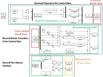
To investigate the accuracy of the H-frame XY positioning system, the desired circle trajectory of the end-effector and the angle rotation of the motors were computed using the Matlab Simulink Desktop Real-Time software and sent to the control box. The position of the end-effector was then recorded by the wireless pen mouse and mouse table. The program Simulink is shown in Fig. 5. The diameter of the circle trajectory was 80 mm and the time to draw it was ~36 s.

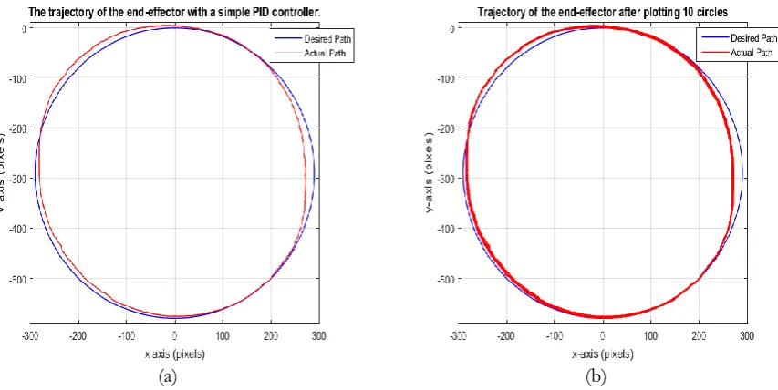
The position of the end-effector and the desired trajectory are compared in Fig. 6(a), where the actual trajectory (red-line) of the end-effector did not completely overlay the desired trajectory (blue-line). The trajectory of the end-effector after drawing a circle ten times is shown in Fig. 6(b), where each trajectory was almost coincident, and so the reproducibility of the system was good.

(a) (b)

Fig. 6. The trajectory of the end-effector with a simple PID controller after drawing (a) one and (b) ten circles.

To see the error of each axis of the system, the root mean square error (RMSE) of each axis and each trajectory were computed, and are summarized in Table. 1. The standard deviations of RMSE of the x-axis and y-axis were very small, confirming that the repeatability of the system is good, but the mean RMSE was high. Thus, a simple PID controller with encoder feedback may be not suitable for this system, and so in Section 4 a technique to improve the accuracy and reduce the mean RMSE of the system is presented.

Table 1. Root mean square error (RMSE) of 10 trajectories.

RMSE (Pixels)a _{x-axis y-axis}

Mean of RMSE 12.76 6.05 Standard Deviation of RMSE 0.44 1.09 Maximum RMSE 24.73 17.41 a_{Note: 1 millimeter is approximately 7 pixels.}

4.

System Control

The pre-test results (Section 3) revealed that the system had a good repeatability, and so the mean RMSE can be compensated by constant and adaptive gain controls. Based on the model described in section 2.2, due to the friction, elastic transmission effect and so on, the relationship between the measured and desired position can be modeled with a nonlinear equation, as shown in Eq. (4):

[

] ( ̇ ̇ ̈ ̈ ) (4)

where and are the measured position which is obtained by the wireless pen mouse and mouse table, and are the desired position or input position, and are the actual position of the end-effector, and is the time. To make the problem simple, Eq. (4) may be simplified to a linear measurement equation as Eq. (5):

[

] [

where is the matrix in . If the matrix, , is an identical matrix, then and . However, is not an identical matrix and so to make the measurement position equal to the desired position a new desired position is given by Eq. (6):

[ ] [ ] [ ] [ ] [ ] (6)

where and are the new desired position or new input position, and is the inverse matrix of . Thus, the inverse matrix ( ) should be estimated.

4.1. Constant Gain Control

The parameters, , , , and can be estimated by the linear least squares algorithms [18, 19]. The linear least squares equation is defined by Eq. (7):

̂ ( ) _{̃ (7)}

where ̂ is the estimated parameter vector, ̃ is the measured vector, and is a matrix shown in Eq. (8):

̂ [ ], ̃ [ ( ) ( ) ( ) ( ) ( ) ( )] , [ ( ) ( ) ( ) ( ) ( ) ( ) ( ) ( ) ( ) ( ) ( ) ( )] (8)

Note: ̃ is the measured vector of the desired position because the measurement of the position should be equal to the desired position.

By using the desired trajectory data and the measurement position of the end-effector (Section 3), the parameters , , , and can be estimated. Then, the feedforward input equation is defined by Eq. (9): [ ] [ ] [ ] [

] (9)

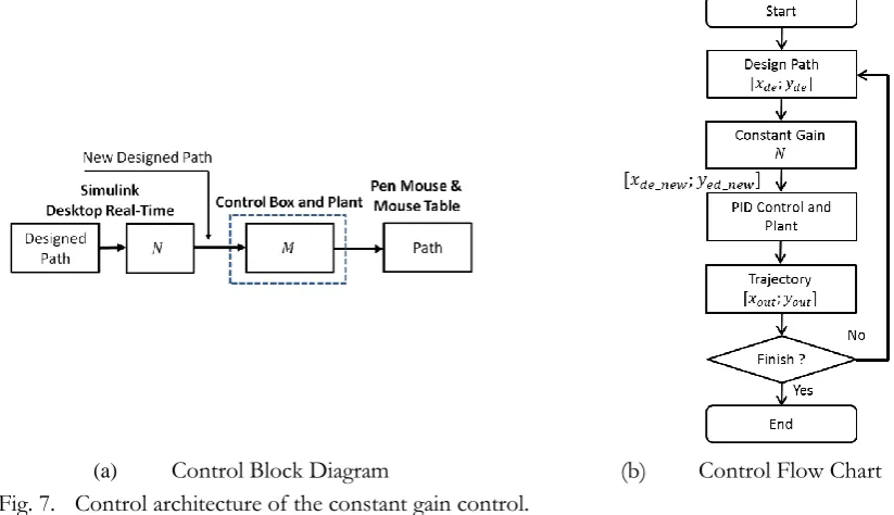
The architecture of the constant control gain is shown in Fig. 7, and the design path presented in Section 3 (an 80 mm diameter circle) was then used to evaluate the controller.

(a) Control Block Diagram (b) Control Flow Chart Fig. 7. Control architecture of the constant gain control.

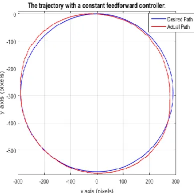
without the constant gain controller, and so the constant gain controller could increase the accuracy of the system.

Fig. 8. The trajectory of the end-effector with a constant gain controller.

Table 2. RMSE of the trajectory with a constant gain controller.

RMSE (Pixels) x-axis y-axis

RMSE 10.71 3.86

Maximum RMSE 20.41 9.55

4.2. Adaptive Gain Control

In this case, the relationship between the actual (measured) and desired position was modelled with a linear time-varying model, as in Eq. (10):

[

] ( ) [

] (10)

where ( ) is a varying matrix. Then, the adaptive gain equation becomes Eq. (11):

[

] ( ) [

] [

( ) ( ) ( ) ( )] [

] (11)

where ( ) is a varying inverse matrix of ( ). The inverse matrix ( ), can be estimated from the recursive least squares (RLS) algorithm [20, 21], which can be formulated in the parameter identification form shown in Eq. (12):

̃( ) ( ) ̂( ) ( ) (12)

where ̃( ) is the measured output, ( ) is the input regression vector, ̂( ) is the vector of estimated parameters, and ( ) is the identification error between the measured output ̃( ) and estimated value

( ) ̂( )

The RLS algorithm was used to iteratively update the unknown parameter vector at each sampling time by using the past input ( , ) and past output ( , ) from the wireless pen mouse and mouse table and the input regression vector . The RLS updates the unknown parameters so as to minimize the sum of the squares of the modeling errors [20, 21]. The RLS algorithm is presented as follows. From Eq. (13):

( ) ̃( ) ( ) ̂( )

( ) [ ( ) ( )] [

]

[ ( ) ( ) ( ) ( )]

(13)

( ) ( ) ( )

( ) ( ) ( ) (14)

where ( ) is the covariance matrix. The calculation of the covariance matrix is defined by Eq. (15):

( ) [ ( ) ( ) ( ) ( ) ( )

( ) ( ) ( ) ] (15)

where is the forgetting factor. Finally, the updated parameter vector, ̂( ), is given by Eq. (16):

̂( ) ̂( ) ( ) ( ) (16)

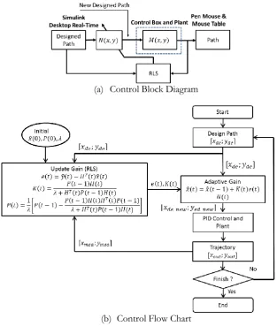
The parameter, , in Eq. (14-15) is the forgetting factor which reduces the influence of the old data which may no longer be relevant to the model. It also prevents a covariance windup problem. From , the parameter vector ( ̂( )) can quickly track changes in the model. Normally, the value of is between 0.9 and 1. A small value of means the contribution of the previous samples is small and the parameters converge quickly, whereas a large value of will increase the sensitivity of the estimation to noise and may cause the parameter estimates to become oscillatory. Thus, with an appropriate value of a fast tracking ability and immunity to noise can be optimized. The architecture of the adaptive gain control is shown in Fig. 9.

(a) Control Block Diagram

(b) Control Flow Chart

Fig. 9. Control architecture of the adaptive gain control.

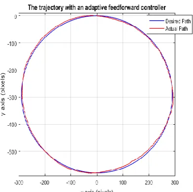
Fig. 10. The trajectory of the end-effector with an adaptive gain controller.

Table 3. RMSE of the trajectory with an adaptive gain controller.

RMSE (Pixels) x-axis y-axis

RMSE 8.21 2.83

Maximum RMSE 14.33 5.83

The circle drawing was complete within ~38 s with the simple PID controller, which was slightly slower than with the constant or adaptive feedforward controllers at ~36 s (Fig. 11). The adaptive gain control was the most efficient at reducing the RMSE of drawing the circle, where it reduced the RMSE by 32.7% and 53.2% on the x-axis and y-axis, respectively, compared to only 16.1% and 36.2% on the x-axis and y-axis, respectively, with the constant gain control (Table 4).

Fig. 11. Comparison of the time to complete drawing a circle of each controller.

Table 4. Comparison of the percentage of RMSE reduction.

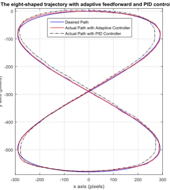
For a more complex pattern test, Fig. 12 shows an example of drawing a figure eight-shaped trajectory with the adaptive feedforward controller and PID controller, where the trajectory with the adaptive feedforward controller was closer to the designed trajectory than the trajectory with the PID controller.

Fig. 12. The trajectory of the end-effector with an adaptive gain controller or a PID controller.

5.

Conclusions

A two-axis, parallel, H-frame XY positioning system (H-Bot) was developed due to the demand for industrial applications. However, the system has an uncertainty of cart or end-effector position when operated at high speed because of the friction and flexibility of the elastic timing belt. Thus, a controller was developed to increase the accuracy of the system. The results revealed that the PID or, especially, the adaptive gain controllers can reduce the RMSE between the desired and the actual trajectory. The constant gain PID control reduced the RMSE by 16.1% and 36.2% on the x-axis and y-axis, respectively, when drawing an 80 mm diameter circle, whereas the adaptive gain control was the most efficient, reducing the RMSE by 32.7% and 53.2% on the x-axis and y-axis, respectively, for drawing the same circle. Also, the actual path of the end-effector was almost coincident to the desired path.

Acknowledgments

Item Sponsored by Ratchadaphiseksomphot Endowment Fund Chulalongkorn University: R/F_2559_002_01_21.

References

[1] K. S. Sollmann, M. K. Jouaneh, and D. Lavender, “Dynamic modeling of a two-axis, parallel, H-frame-type XY positioning system,” IEEE/ASME Transactions on Mechatronics, vol. 15, no. 2, pp. 280-290, 2010.

[2] K. Kim, K. Yoon, J. Suh, and J. Lee, “Laser scanner stage on-the-fly method for ultrafast and wide area fabrication,” Physics Procedia, vol. 12, pp. 452-458, 2011.

[3] K. Suzuki and N. Suzuki, “Large gantry table for the 10th generation LCD substrates,” Technical Review No. 76, NTN Global, 2008.

[4] L. Assoufid, N. Brown, D. Crews, J. Sullivan, M. Erdmann, J. Qian, and D. J. Merthe, “Development of a high-performance gantry system for a new generation of optical slope measuring profilers,”

[5] K. Ito, M. Yamamoto, M. Iwasaki, and N. Matsui, “Fast and precise positioning of ball screw-driven table system using minimum jerk control-based command shaping,” in Advanced Motion Control, 2006. 9th IEEE International Workshop on, IEEE, 2006, pp. 115-119.

[6] P. Pitakwatchara, “Design and analysis of a two-degree of freedom cable driven compound joint system,” presented at The Second TSME International Conference on Mechanical Engineering, 2011.

[7] S. Weikert, R. Ratnaweera, O. Zirn, and K. Wegener, “Modeling and measurement of h-bot kinematic systems,” presented at American Society for Precision Engineering, Denver, CO, 2011.

[8] A. Zaki, K. Sollmann, M. Jouaneh, and E. Anderson, “Nonlinear control of a belt driven two-axis positioning system,” in ASME 2008 International Mechanical Engineering Congress and Exposition, American Society of Mechanical Engineers, 2008, pp. 807-814.

[9] K. S. Sollmann, “Modeling, simulation, and control of a belt driven, parallel H-frame type two axis positioning system,” Master’s thesis, Univ. Rhode Island, Kingston, RI, 2007.

[10] R. Ratnaweera, “Integration of a Cartesian robot,” Master’s thesis, Swiss Federal Institute of Technology ETH Zurich, 2010.

[11] A. S. Kulkarni and M. A. El-Sharkawi, “Intelligent precision position control of elastic drive systems,”

Energy Conversion, IEEE Transactions on, vol. 16, no. 1, pp. 26-31, 2001.

[12] T. S. S. Jayawardene, M. Nakamura, and S. Goto, “Accurate control position of belt drives under acceleration and velocity constraints,” International Journal of Control Automation and Systems, vol. 1, pp. 474-483, 2003.

[13] M. Feemster, P. Vedagarbha, D. M. Dawson, and D. Haste, “Adaptive control techniques for friction compensation,” Mechatronics, vol. 9, no. 2, pp. 125-145, 1999.

[14] P. Vedagarbha, D. M. Dawson, and M. Feemster, “Tracking control of mechanical systems in the presence of nonlinear dynamic friction effects,” Control Systems Technology, IEEE Transactions on, vol. 7, no. 4, pp. 446-456, 1999.

[15] A. Hace, K. Jezernik, and A. Šabanović, “SMC with disturbance observer for a linear belt drive,”

Industrial Electronics, IEEE Transactions on, vol. 54, no. 6, pp. 3402-3412, 2007.

[16] ATMEL, 8-Bit AVR Microcontrollers, AVR221: Discrete PID Controller. ATMEL Corporation, 2006. [17] G. F. Franklin, J. D. Powell, and M. L. Workman, Digital Control of Dynamic System, vol. 3. Menlo Park:

Addison-Wesley, 1998.

[18] J. L. Crassidis and J. L. Junkins, Optimal Estimation of Dynamic Systems. CRC press, 2011.

[19] D. Simon, Optimal State Estimation: Kalman, H Infinity, and Nonlinear Approaches. John Wiley & Sons, 2006.

[20] R. Rajamani, N. Piyabongkarn, J. Lew, K. Yi, and G. Phanomchoeng, “Tire-road friction-coefficient estimation,” IEEE Control Systems, vol. 30, no. 4, pp. 54-69, 2010.