estimation
.
White Rose Research Online URL for this paper:
http://eprints.whiterose.ac.uk/3597/
Article:
Gotoh, Y., Hochberg, M.M. and Silverman, H.F. (1998) Efficient training algorithms for
HMMs using incremental estimation. IEEE Transactions on Speech and Audio Processing,
6 (6). pp. 539-548. ISSN 1063-6676
https://doi.org/10.1109/89.725320
[email protected] https://eprints.whiterose.ac.uk/ Reuse
Unless indicated otherwise, fulltext items are protected by copyright with all rights reserved. The copyright exception in section 29 of the Copyright, Designs and Patents Act 1988 allows the making of a single copy solely for the purpose of non-commercial research or private study within the limits of fair dealing. The publisher or other rights-holder may allow further reproduction and re-use of this version - refer to the White Rose Research Online record for this item. Where records identify the publisher as the copyright holder, users can verify any specific terms of use on the publisher’s website.
Takedown
If you consider content in White Rose Research Online to be in breach of UK law, please notify us by
IEEE TRANSACTIONS ON SPEECH AND AUDIO PROCESSING, VOL. 6, NO. 6, NOVEMBER 1998 539
Efficient Training Algorithms for
HMM’s Using Incremental Estimation
Yoshihiko Gotoh,
Member, IEEE,Michael M. Hochberg,
Member, IEEE,and Harvey F. Silverman,
Fellow, IEEEAbstract— Typically, parameter estimation for a hidden Markov model (HMM) is performed using an expectation-maximization (EM) algorithm with the maximum-likelihood (ML) criterion. The EM algorithm is an iterative scheme that is well-defined and numerically stable, but convergence may require a large number of iterations. For speech recognition systems utilizing large amounts of training material, this results in long training times. This paper presents an incremental estimation approach to speed-up the training of HMM’s without any loss of recognition performance. The algorithm selects a subset of data from the training set, updates the model parameters based on the subset, and then iterates the process until convergence of the parameters. The advantage of this approach is a substantial increase in the number of iterations of the EM algorithm per training token, which leads to faster training. In order to achieve reliable estimation from a small fraction of the complete data set at each iteration, two training criteria are studied; ML and maximum a posteriori (MAP) estimation. Experimental results show that the training of the incremental algorithms is substantially faster than the conventional (batch) method and suffers no loss of recognition performance. Furthermore, the incremental MAP based training algorithm improves performance over the batch version.
Index Terms— HMM training algorithm, incremental estima-tion, MAP estimation.
I. INTRODUCTION
T
HE HIDDEN Markov model (HMM) is a standard tool used in speech recognition processing. The HMM repre-sents a statistical model of a speech signal (given a certain data set) and its utility stems from the fact that the parameters can be easily learned from training data. In most HMM systems, training is performed using the maximum-likelihood (ML) criterion with the expectation-maximization (EM) algorithm [1]. The EM algorithm for HMM’s is simple, well-defined, and numerically stable, but often convergence can be slow. Because speech signals can differ substantially for various acoustic environments (e.g., talkers, tasks, channels, etc.), it is a fundamental requirement that the training process estimates the HMM parameters in the most appropriate way. RobustnessManuscript received April 29, 1996; revised November 21, 1997. This work was supported in part by the National Science Foundation under Grants MIP-9120843 and MIP-9509505 and by Wernicke ESPRIT Project (BRA 6487). The associate editor coordinating the review of this manuscript and approving it for publication was Prof. John H. L. Hansen.
Y. Gotoh is with the Department of Computer Science, University of Sheffield, Sheffield S1 4DP, U.K. (e-mail: [email protected]).
M. M. Hochberg is with Nuance Communications, Menlo Park, CA 94025 USA (e-mail: [email protected]).
H. F. Silverman is with LEMS, Division of Engineering, Brown University, Providence, RI 02912 USA ([email protected].).
Publisher Item Identifier S 1063-6676(98)07787-6.
to environment is typically achieved through increasing the size of the training data set so that most variation is observed. This further slows the process of training HMM systems. This paper presents an incremental estimation approach to speed-up the training of HMM’s without any loss of recognition performance.
A. Background
Given a training data set, the EM algorithm iteratively estimates the HMM parameters in two stages; an expectation step (E-step) followed by a maximization step (M-step). In-stead of performing the maximization directly, the sample data is augmented with latent information (e.g., the hidden state sequence) so that the maximization process becomes more tractable. There have been a number of proposed methods for reducing the amount of computation required for this process. One of the most common approaches uses Viterbi training [2] instead of the full forward-backward approach. This approach, however, may cause some degradation in recognition performance.
The use of incremental training (i.e., using only subsets of the training data at each iteration) is common in gradient-based learning methods (e.g., backpropagation training of connectionist systems [3], [4]). Recently, Neal and Hinton have discussed a theoretical justification for implementing an incremental E-step for ML estimation [5]. Their rationale is stated as follows.
If the statistics for the E-step are incrementally collected and the parameters are frequently estimated, it should speed the convergence because the information from the new data contributes to the parameter estimation more quickly than the standard algorithm.
They reported a substantial speed-up in convergence for a mixture estimation problem using such an incremental EM algorithm. In the work presented here, it was hoped that speed improvements could be obtained by applying a similar technique to HMM training.
It should be noted that there has been other research into the use of incremental algorithms for HMM’s. Namely, Krishna-murthy et al. [6] investigated an HMM-based sequential signal processing scheme where the stochastic approximation method was used to maximize the Kullback–Leibler (KL) information measure [7]. Their simulation study suggested significant improvements in convergence. Also, Baldi, Chauvin and others have worked on on-line training of HMM’s for applications in computational molecular biology [8], [9]. Fast convergence of
an incremental generalized EM algorithm was also noted by Jordan and Jacobs in their work on hierarchical mixtures of experts [10]. On a related note, Huo and Lee have developed similar approaches to those developed here, but have focused primarily on the problem of on-line adaptation [11].
B. General Approach
This paper presents several related approaches to HMM training based on incremental variants of the EM algorithm. The general approach of these algorithms is to select a subset of data from the training set, update the model parameters based on the subset, and then iterate the process until con-vergence of the parameters. The approaches are considered incremental because, at each iteration, the HMM parameters are adjusted before all the training data has been processed. This training strategy contrasts sharply to the standard batch training method where the model is updated only after all the data in the training set are processed.
In the case of parameter estimation for a complex model from limited training data, it can be very easy to overfit the model to the training data. The dilemma faced by the incremental algorithms is to achieve reliable parameter esti-mation from a small fraction of the entire data set at each iteration. This leads to a number of different approaches based on ML and maximum a posteriori (MAP) estimation. Section II presents an incremental ML algorithm that stores the observed information for both the current and the earlier iterations in separate storage blocks, effectively taking a large amount of data into consideration. This approach not only achieves robust estimation, but guarantees stable convergence. Two incremental training algorithms based on MAP estimation are described in Section III. The first approach is similar to the incremental ML approach but utilizes a MAP training criterion. The second MAP approach differs from the ML version in that robust estimation is achieved by accumulating the observed information into the prior parameters. Intuitively, the prior acts as a stabilizer for the training process. A series of experiments (see Section IV) are performed on a talker-independent, connected-alphadigit recognition task. The results show that the convergence of the incremental training algorithm is substantially faster than batch training without any degradation in recognition performance. Furthermore—and rather unexpected, to be honest—the incremental MAP train-ing improves performance over the batch version. The paper concludes with a discussion of the incremental approaches and a listing of the pros and cons.
II. INCREMENTAL ML ESTIMATION
This section presents an approach to incremental ML es-timation of HMM parameters. The salient features of both the standard EM algorithm and its incremental variant are summarized. Throughout this paper, an exponential-family distribution is assumed (standard practice for HMM’s) and leads to an extremely simple algorithm employing the concept of sufficient statistics.
Let be a sample of observed information (or incomplete
data) and assume that there exists a mapping , where
is the latent information (or missing data). Given , the EM algorithm maximizes the likelihood over in a parameter space by exploiting the relation
(1)
Suppose that the complete data joint likelihood has the regular exponential family form [12], [13], i.e.,
(2)
where implies the transpose, is the set of parameters, and is the complete data sufficient statistics1of fixed
dimension . Both and are given by dimensional
column vectors. Also, is a real-valued function of and , and is a normalization factor given by
(3)
A. Standard EM Algorithm
The standard EM algorithm is a procedure that iteratively estimates parameters using the ML criterion. The following two-stage procedure computes a th iteration for an exponen-tial family distribution [12]:
E-step: Given and estimate the complete data sufficient statistics from
M-step: Set the new estimate of to the solution of
(4)
where the expectations are computed by
At each iteration, the complete data sufficient statistics are computed over a fixed data set and then the model parameters are estimated from the sufficient statistics so that the likelihood is maximized. This approach is referred to as the batch ML algorithm in the experiments. The algorithm is considered memoryless because the sufficient statistics are only collected within an iteration. The algorithm is attractive because the likelihood increases monotonically and stable convergence is guaranteed [12].
1A sufficient statistic is a function of the data which represents the information needed to estimate the parameters of the distribution. For a typical example, consider a joint normal distribution
f(x j ~; 6) T
t=1
exp 01
2(~xt0 ~)3601(~xt0 ~)
for data set x = f~xtgt=1;...;T. It has a sufficient statistic S =
f T
t=1~xt; Tt=1~x2tg. The mean and the covariance of the distribution,
~ and 6, can be estimated from S. In standard HMM training terminology,
GOTOH et al.: TRAINING ALGORITHMS FOR HMM’S 541
B. Incremental Variant
The incremental variant is applicable when the observed
data are independent. In this approach, the
data are separated into subsets and then processed incremen-tally in the computation. The incremental ML algorithm can be implemented as follows [5]. Let be the sufficient statistic associated with the sample data :
E-step: Choose some data to be processed.
For fixed compute
Then, compute the complete data sufficient statistic
M-step: Set the new estimation to the solution of
(5)
Neal and Hinton have shown that stable convergence2 is guaranteed for this approach [5].
Fig. 1 compares the computational flows for the batch and incremental ML algorithms. Both algorithms share the same M-step, but differ in the method of computing the sufficient statistics in the E-step. Given , the batch ML algorithm computes sufficient statistics on the whole data set . The incremental method computes for a selected subset of the data conditioned on . The complete data sufficient statistics are computed by maintaining
the past for and , and accumulating
these values with for use in the M-step.3 Note that the selection of the sample data can be very flexible; for instance, the E-step can be processed on a single data item or on multiple items and/or the selection can be done sequentially or randomly.
Because only a subset of the data is processed for each iteration of the algorithm, the amount of computation re-quired per parameter update can be significantly reduced. The drawback to this approach is that it may cause storage problems when the number of subsets is large. Specifically, the storage requirement is on the order of , where is the number of training subsets and is the number of modeled parameters. This can greatly limit the application of the algorithm to systems with large numbers of parameters (e.g., phone-based, context-dependent HMM’s). A possible way around this problem may be accumulation of the sufficient statistics (see the related footnote of this section). One such method has been proposed where a decay factor is utilized to
forget earlier contributions to the accumulation [5], [10].
2To show stable convergence for the incremental variant, it is sufficient to show thatQ( (p)j (p)) Q( (p+1) j (p)) is satisfied for the standard auxiliary functionQ( j 0) yf(y j x; 0) log f(x; y j ). In [5], Neal and Hinton basically show that this does indeed hold when sample data are assumed independent. This implies that the incremental variant is a generalized EM (GEM) algorithm [12] and that the likelihood will increase monotonically to a (local) maximum.
3The replacementS
t = f(yt j ~xt; (p))St(~xt; yt) and the summation
S(p+1) =
S in algorithm (5) is the “right” approach in a theoretical sense (e.g., stable convergence is guaranteed). However, many alternatives exist and they may provide practical solutions for some cases. One such method is simply accumulating sufficient statistics at each iteration, i.e.,
S(p+1)= S(p)+ St.
C. Incremental ML Training Algorithm for HMM Parameters
The incremental ML variant described above leads to the following HMM training algorithm.
1) Initialization:
• Initialize the HMM parameters .
• Divide the complete training utterances into
disjoint subsets .
• Initialize sufficient statistics appropriately for each subset (e.g., set to zero).
• Initialize the update counter . 2) E-step:
• Choose an utterance subset .
• Given , compute
using forward/backward recursion
over .
• Set sufficient statistics for the whole data set by .
3) M-step:
• Set the new estimate of to the solution of .
4) If no convergence, set and repeat from Step 2. There is a practical consideration in the actual training imple-mentation. Suppose statistics is replaced by after the forward/backward recursion on , then the summation at the E-step can be accomplished by
because is not updated at this iteration.
III. INCREMENTAL MAP ESTIMATION
This section presents incremental MAP estimation ap-proaches for training HMM’s. The resulting model represents a compromise between observed evidence and prior information. In the first approach, a typical MAP formulation is applied; a prior distribution is specified on the parameters and the mode of the posterior distribution determines the parameters. The main focus of this section, however, is on a recursive
Bayes approach [14]. This is a variation of incremental MAP
estimation and is the second approach described in this section. It is similar to incremental ML estimation in that it handles a small subset of data at each iteration and frequently estimates the model parameters. It is different in that it keeps track of previous data through an evolving prior. As a consequence, it does not maintain the relevant statistics on the fixed data set, but has the advantage that it uses a fixed amount of storage for any subset size.
A. MAP Estimation via the EM Algorithm
The posterior probability density function (pdf) is calculated by Bayes’ rule as
(6)
where is the likelihood for the observed data and denotes the prior pdf of the parameter . The prior parameter represents the information known a
first requires computing the marginal density (which can be very expensive). If the posterior pdf has the same
functional form as (i.e., where
is the posterior parameter), then the pdf belongs to the conjugate family of distributions.4 This paper makes use of a conjugate prior because it leads to simple methods for computing the mode of the posterior pdf’s.
The EM algorithm provides an iterative solution for estimat-ing the MAP parameters [12]. The extension of the standard ML approach (4) or its incremental variant (5) is nearly trivial. Suppose the complete data joint likelihood
has the regular exponential family form as in (2), then the following M-step for MAP estimation replaces that for ML-based algorithms:
M-step: Set the new estimation to the solution of
Note that the E-steps in (4) and (5) are unchanged. For each iteration, the batch (or the incremental) MAP algorithm com-putes the complete data sufficient statistics over whole data set (or subset data), then estimates the model parameters from the sufficient statistics and the prior parameters so that the posterior probability is maximized. When the sufficient statistics are strictly maintained, the posterior probability—not necessarily the likelihood—improves monotonically for both the batch and the incremental MAP approaches.5
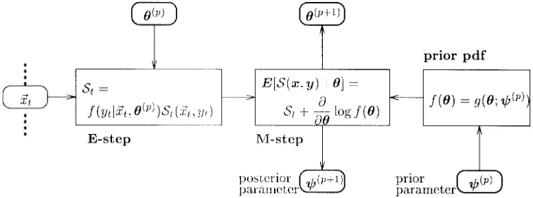
B. Recursive Bayes Approach
In the previously described incremental approaches, the contribution of the complete data set was represented by storing the sufficient statistics in separate memory blocks. This can cause problems with the amount of required mem-ory. A proposed solution utilizes a variation on the recur-sive Bayes approach for performing sequential estimation of model parameters given incremental data [14]. Denote where is drawn from the whole data
set and the sample data are independent.
By the recursive Bayes formula
(7)
or simply
(8)
where indicates proportionality, is the prior pdf, and . The recursive Bayes approach results in a sequence of prior pdf’s
and a corresponding sequence of MAP estimates given by
(9)
Recall that the conjugate prior pdf, defined by , results in the the posterior pdf with the same functional form
4Methods for handling the conjugate prior are well developed and can be found in most textbooks on Bayesian statistics, e.g., [15]–[17].
5The M-step expression is derived from Bayes’ rule (6) and is equivalent to the formulation specified in [12]. The theoretical considerations of the convergence property (for the posterior probability) are the same as for the ML case.
where and are the prior and posterior parameters. In this case, the recursive Bayes approach also pro-duces a sequence of prior parameters
which act as the memory for the previously observed infor-mation. Note that if is a noninformative prior, then (9) gives an ML estimate of .
The incremental (iterative) MAP estimation process can be combined with the recursive Bayes approach. Assuming the regular exponential family form (2) for the joint likelihood, the recursive Bayes approach estimates the model parameters in the following two-stage procedure.
E-step: Choose a data to be processed.
For fixed compute
M-step: Given set the new
estimate of to the solution of
Also find the posterior parameter
(10)
By using the conjugate prior pdf, the posterior naturally becomes the prior for the next iteration. Gauvain and Lee have presented the expressions for computing the posterior distributions and MAP estimates of continuous density HMM parameters [18]. Due to space limitation, the reader is directed to [18] for the HMM formulations of (8) and (9).
In comparison with the incremental ML method in Section II, the difference is evident in handling the relevant statistics. After computing for a selected subset, Algorithm
(5) does the summation at the E-step. Thus,
the complete data sufficient statistics condition is satisfied when estimating parameters at the M-step. On the other hand, Algorithm (10) directly accumulates into the prior at the M-step.
Fig. 2 illustrates the computational flow for the recursive Bayes approach. The approach handles a small subset of data at each iteration and frequently estimates the model parameters from the posterior. This variant no longer assumes a “fixed data set” and thus does not keep the relevant statistics in a strict sense. As a consequence, the monotone convergence property no longer holds. There are, however, a number of advantages to this approach:
• the training set can be modified during training (e.g.,
on-line training);
• the storage requirements for the algorithm are reduced because it does not require storing the sufficient statistics for each subset.
In addition, empirical results indicate that the algorithm does converge to a useful solution.
C. Recursive Bayes Training Algorithm for HMM Parameters
The recursive Bayes approach leads to the following HMM training algorithm:
1) Initialization:
• Choose a prior on the HMM
parameters.
GOTOH et al.: TRAINING ALGORITHMS FOR HMM’S 543
Fig. 1. These diagrams compare the computational flow for the batch and incremental ML algorithms. At each iteration, the batch method computes sufficient statisticsS(p+1) on the whole data setx = f~xtgt=1;111;T. On the other hand, the incremental approach computesSt for some data~xt, then accumulates S(p+1) using statistics from past iterations.
Fig. 2. Computational flow for the recursive Bayes approach, a variation to the incremental MAP algorithm. In this approach, only a subset of the data
~xt is used at each iteration and previously observed information is accumulated into the prior parameter .
• Initialize the update counter . 2) E-step:
• Choose an utterance subset .
• Given , compute
using forward/backward recursion
over .
3) M-step:
• Given a prior pdf , set the new
estimate to the solution of .
• Find the posterior parameters .
4) If no convergence, set and go to Step 2.
IV. EXPERIMENTS
[image:6.612.106.494.403.547.2]Fig. 3. Graphs compare the convergence characteristics for discrete observa-tion HSMM’s with Poisson state duraobserva-tions. Log-likelihood and the recogniobserva-tion performance were shown for (a) ML batch training and the incremental ML approaches with (b) three, (c) ten, and (d) 30 subsets. For the “M subsets” case, one pass is completed when the algorithm has iteratedM times and processed each subset.
A. Incremental ML Estimation
Experiments for the incremental ML estimation approach were performed using a discrete observation HSMM with a Poisson distribution on state duration [20]. First, the parame-ters of the HMM were randomly initialized6 and the training utterances were separated into one, three, ten, or 30 subsets (the one subset case is equivalent to batch training). Subsets were then chosen sequentially at each iteration. Fig. 3 shows the log-likelihood (on the training set) and the recognition performance (on the test set) versus the amount of data processed for the various number of subsets. Note that for the “ subsets” case, one pass is completed when the algorithm has iterated times and processed each subset. There are a few points clearly shown in the figure.
• The likelihood and the recognition performance improved faster for the incremental method than for the batch version and the effect was more pronounced when the number of subsets was larger.
• The HMM’s attained about the same performance level, independent of the training method used. The incremental approach did not sacrifice any recognition performance while speeding the convergence.
Table I summarizes the processing time on a Sparc 10–51 workstation for the various subset sizes. The third column shows the time required to process ten full passes of the
6Random initialization of the parameters was performed in a straightforward fashion. The multinomial distribution terms were initialized using a uniform random number generator and the distributions were normalized to sum-to-one. The state-duration mean was randomly selected between (roughly) 20 to 100 ms.
TABLE I
PROCESSINGTIME FORDISCRETEOBSERVATIONHSMM’sWITHPOISSONSTATE DURATIONS ON ASPARC10–51 WORKSTATION. THERESULTSARE FORML BATCHTRAINING(.i.e., SINGLESUBSETCASE)AND THEINCREMENTALML APPROACHES WITHTHREE, TEN,AND30 SUBSETS. “TOTENPASSES” INDICATES
PROCESSING3484 UTTERANCESTENTIMES AND“TO84% LEVEL” INDICATESREACHINGTHISLEVEL OFRECOGNITIONPERFORMANCE
training data (34 840 utterances in total). An interesting ob-servation is that the incremental ML approach decreased this processing time by more than 20% over the batch version. This improvement is the result of more effective pruning of unlikely state sequences at earlier stages in the training. The incremental algorithms are able to refine and apply their model parameters well before the batch algorithm.7
The speed improvement of the incremental ML approach is also demonstrated by the CPU time required to reach a recognition accuracy of 84% (fourth column of Table I). The batch training (i.e., the single subset case) required five passes at a cost of 9.1 h of CPU time. The incremental ML with ten subsets required 1.8 passes and 2.7 CPU h. These numbers account for savings of about a factor of 2.8 in the number of utterances that need to be processed and a factor of 3.4 in processing time. It is expected that slightly better speed improvements are attainable using greater than 30 subsets. Implementing this becomes difficult, however, because the approach needs separately maintained sufficient statistics for each subset (see Section II-B).
B. Recursive Bayes Estimation
Experiments for the recursive Bayes estimation—a variation to the incremental MAP approach—focused on the estima-tion of tied-mixture, continuous density HMM parameters, because this problem had such high computational costs. In addition, there were reasonable methods for generating the prior distributions.
1) Prior Parameter Generation The initial tied-mixture parameters were derived from the discrete observation HSMM which used a Poisson distribution to model state duration. This model was then converted to a tied-mixture model by simply replacing each discrete symbol with suitable parameters for a multivariate normal distribution. Normal means and full covariances were estimated from the training data. Given the above approach, a reasonable method to initialize the prior was to set the prior parameters such that the mode of the distribution corresponded to the initial HMM parameters. The employed prior distributions were the normal–Wishart distribution for the parameters of the normal distribution and the Dirichlet distribution for the rest of model parameters [15].
GOTOH et al.: TRAINING ALGORITHMS FOR HMM’S 545
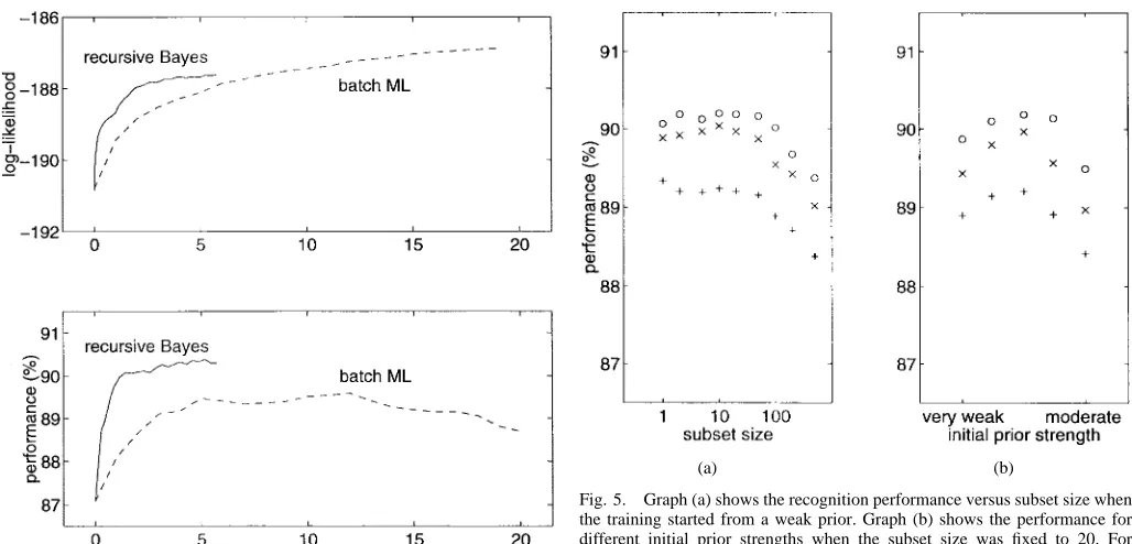
Fig. 4. Comparison of speed of convergence between the batch ML (dashed line) and the recursive Bayes training with a subset size of 20 utterances (solid line). One full pass is equivalent to one iteration for the batch ML method, and approximately to 175 iterations for the recursive Bayes approach.
The prior strength8—interpreted as the amount of observed data required for the posterior to significantly differ from the prior—was determined empirically. A subjective mea-sure of prior strength was used where a very weak prior was (almost) equivalent to a noninformative prior and a very strong prior (almost) corresponded to impulses at the initial parameter values. The Poisson duration parameters were estimated from the multinomial parameters using the system equation approach and the evidence accumulated to the Dirichlet prior parameters [21]. The rest of the model parameters—including the transition and mixture observation parameters—were estimated using the expressions given by Gauvain and Lee [18].
2) Speed of Convergence: In this experiment, the speed of
convergence for the incremental training was compared with that of standard batch ML training. For both approaches, the tied-mixture parameters were initialized identically as described above. The recursive Bayes training started from a relatively weak prior and iterated the model estimation algorithm using a subset size of 20 randomly-selected ut-terances.9 Fig. 4 shows the log-likelihood (on the training set) and the recognition performance (on the test set) as a function of the amount of utterances processed. Unlike
8In this experiment, initial prior parameters were derived from the sufficient statistics accumulated from 3484 utterances (byproduct of conventional ML training in Section IV-A). The prior strength was decided by simply multiply-ing some factor to the accumulation. When 100% level of accumulation was used for the prior, the new training data did not affect the recursive Bayes parameter estimation very much; thus, it was referred to as the strong prior. Similarly, the moderate, weak, and very weak priors were set approximately to the 10%, 1%, and 0.1% level of accumulation.
9Random selection was done in order to avoid possible bias in arrangement of training utterances.
[image:8.612.43.557.55.302.2](a) (b)
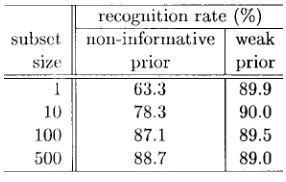
Fig. 5. Graph (a) shows the recognition performance versus subset size when the training started from a weak prior. Graph (b) shows the performance for different initial prior strengths when the subset size was fixed to 20. For both cases, “+,” “2,” and “” denote performances achieved after processing 2000, 4000, and 10 000 utterances, respectively.
the conventional EM algorithm that guarantees monotone likelihood improvement, the recursive Bayes approach does not possess this nice property at each update. However, it is still possible to observe the global trend of the likelihood by computing the running average of the past values. Here, the past 175 likelihoods (approximately equivalent to the number of utterances processed by the batch training for one iteration) were averaged.
The log-likelihood curves in Fig. 4 show that the batch ML training had not converged after 15 full passes while the recur-sive Bayes algorithm seemed to converge before processing five full passes. The recognition performance is even more interesting. Performance of batch training reached 89.5% after six full passes (processing approximately 21 000 utterances); it remained at this level and then gradually declined. The decline in performance was probably due to overfitting the model to the data. On the other hand, the recursive Bayes algorithm stabilized after slightly more than one pass (processing about 4000 utterances)—a factor of five faster than the batch al-gorithm—to an even higher level of performance. Because the overhead of the incremental processing is negligible when compared with the batch training, the reduction in the total number of utterances processed is directly reflected in the training time. The fact that the algorithm converges after 4000 utterances (i.e., 200 iterations) is not surprising because the prior/posterior terms in the MAP estimator become stronger and stronger with each update. As training progresses, each subsequent update has less of an effect.
3) Improvement of Performance: In the second set of
TABLE II
PROCESSINGTIME FOR THEFIRST1000 UTTERANCES ON ASPARC10–51 WORKSTATION FORDIFFERENTNUMBERS OFUTTERANCES IN THESUBSETS
started from a weak prior and the performances achieved after processing 2000, 4000, and 10 000 utterances were plotted. The best performance (90.4%) was obtained when the subset size was between 20 and 50. This represents an 8% reduction in the error rate from the batch ML training method. This ap-proach is relatively robust as performance appears independent of subset size for those subsets with less than 50 utterances. However, the performance starts to degrade as the subset size grows beyond 100 utterances.
In Fig. 5(b), the performance of the system for different initial prior strengths is shown. In all cases, a fixed subset size of 20 was used. As can be seen from the figure, the choice of the prior parameter strength does seem to have an effect on the performance, i.e., there exists some appropriate prior strength factor that most enhances the performance. Note that, when the initial prior is stronger, the result was less affected by the subset size. The effect of the prior strength may not be significant as more utterances are processed.
4) Processing Time: Table II shows the CPU time required
to process 1000 utterances for different subset sizes. The recursive Bayes training started from a relatively weak prior. The table shows a very slight increase in processing time as fewer utterances were processed per subset. The reason is that the parameter estimation computation (M-step) was insignificant compared with the computation of the normal mixtures for each utterance (E-step). Thus, the processing time is nearly proportional to the total number of utterances and independent of the subset size (and, needless to say, independent of the prior strength).
5) Variation—Noninformative Prior: One variation of the
recursive Bayes approach is to use a noninformative prior. This is similar to the incremental ML method10 described in Section II in that both approaches estimate the model parameters solely from the data. The difference is that the incremental ML maintains the relevant statistics for indi-vidual subsets separately and sums them when estimating the model parameters, while the recursive Bayes training with the noninformative prior accumulates them into the prior parameters. Table III shows the recognition performances after 4000 utterances for recursive Bayes training with a noninformative prior versus that with a weak prior. The noninformative prior implies a “zero” strength factor. For both approaches, not only were the model parameters initialized to identical values, but the same training method was also used. The difference in the recognition rate after the training suggests the importance of prior parameters. It is hypothesized that the prior acts to keep the early models from overfitting the initial subset data.
10Naming of the approach—either incremental ML or recursive Bayes—is a matter of convention. In fact, Neal and Hinton [5] and Jordan and Jacobs [10] referred to this (i.e., the recursive Bayes approach with the noninformative prior) as a modified incremental ML method.
TABLE III
RECOGNITIONPERFORMANCESAFTER4000 UTTERANCES FORRECURSIVEBAYES TRAINING WITH ANONINFORMATIVEPRIORVERSUSTHAT WITH AWEAKPRIOR
V. SUMMARY AND DISCUSSION
This paper has presented two approaches (utilizing the ML and the MAP criterion) to incremental estimation of HMM parameters. Both approaches process only a small subset of the training data at each iteration, which leads to frequent updating of the model parameters. Experimental results have shown that the approaches substantially reduce the HMM training time without sacrificing recognition performance. Specifically, for recursive Bayes training of a continuous density HMM, it was found that the approach also improved the recognition performance over conventional ML. A possible reason for the performance improvement may be due to accumulation of the priors for infrequently observed events. This may provide a smoothing of the parameter estimates which reduces the effect of overfitting.
It was found that the existence of the prior (and, as a consequence, the use of MAP estimation) is an important factor when the HMM parameters are estimated frequently from a very small amount of data. Even a very weak prior works far better than does the noninformative prior case. Intuitively, the prior must be strong enough to keep the model from overfitting the data at the early stages of training. However, the prior must be weak enough so that the data can be effectively modeled at later stages of training.
A. Pros and Cons for the Incremental Algorithms
The two incremental algorithms share similar concepts in many respects and, thus, result in similar performance. However, there exists a clear difference in handling the observed information. Specifically, the incremental ML al-gorithm maintains the relevant statistics from the individual subsets separately (physically in separate memory blocks), while the recursive Bayes accumulates them into the prior parameters. This difference characterizes one approach from the other in the following manner.
GOTOH et al.: TRAINING ALGORITHMS FOR HMM’S 547
• One possible drawback for incremental ML is that this approach may cause a storage problem because it main-tains the statistics separately for individual subsets. This is especially true for the case where the number of model parameters and/or the number of subsets is very large. As a consequence, an experiment with more than 30 subsets was not performed, although it was expected that further speed improvements were possible. On the other hand, recursive Bayes keeps the information as the prior parameters (i.e., one place) and utilizes a fixed amount of storage regardless of subset size.
• Continuous density HMM training by the ML method tended to overfit to the training data. Because conver-gence of the log-likelihood was not very apparent, it was difficult to determine an appropriate stopping condition for the training. On the other hand, the log-likelihood by the recursive Bayes approach showed clear convergence due to the increasing amount of information in the prior parameters. Furthermore, the recognition performance reached an even higher level than the standard batch version.
Thus far, the comparison seems to indicate that the recur-sive Bayes estimation approach is more attractive than its incremental ML counterpart. It does not suffer from storage problem and its slightly weak theoretical underpinning does not seem to cause any trouble. It even leads to improved performance. However, it is not a panacea either.
• Unlike the ML method, MAP estimation requires a prior pdf when the training begins. It was found that the performance of the recursive Bayes approach was greatly dependent on the choice of prior—which is often very difficult to make and is probably a task-dependent issue. If a reasonable method is known for preparing the prior (as in the tied-mixture HMM training case), then incremental MAP (or recursive Bayes) is certainly the choice over the ML algorithm. On the other hand, if there is no clear scheme for generating the prior, then the incremental ML method provides an alternative solution without requiring a prior that, nevertheless, can achieve far more efficient training than does standard batch training.
REFERENCES
[1] L. E. Baum, T. Petrie, G. Soules, and N. Weiss, “A maximization technique occurring in the statistical analysis of probabilistic functions of Markov chains,” Ann. Math. Stat., vol. 41, pp. 164–171, 1970. [2] C. J. Wellekens, “Mixture density estimators in Viterbi training,” in
Proc. ICASSP’92, San Francisco, CA, Mar. 1992, vol. 1, pp. 361–364.
[3] H. A. Bourlard and N. Morgan, Connectionist Speech Recognition: A
Hybrid Approach. Boston, MA: Kluwer, 1994.
[4] N. Morgan and H. Bourlard, “Continuous speech recognition,” IEEE
Signal Processing Mag., vol. 12, pp. 25–42, May 1995.
[5] R. M. Neal and G. E. Hinton, “A new view of the EM algorithm that justifies incremental and other variants,” submitted to Biometrika, 1993. (available on-line at
ftp://ftp.cs.utoronto.ca/pub/radford/em.ps.Z.) [6] V. Krishnamurthy and J. B. Moore, “On-line estimation of hidden
Markov model parameters based on the Kullback-Leibler information measure,” IEEE Trans. Signal Processing, vol. 41, pp. 2557–2573, Aug. 1993.
[7] E. Weinstein, M. Feder, and A. V. Oppenheim, “Sequential algorithms for parameter estimation based on the Kullback-Leibler information
measure,” IEEE Trans. Acoust., Speech, Signal Processing, vol. 38, pp. 1652–1654, Sept. 1990.
[8] P. Baldi, Y. Chauvin, T. Hunkapiller, and M. A. McClure, “Hidden Markov models in molecular biology: New algorithms and applications,” in Advances in Neural Information Processing Systems, vol. 5, S. J. Hanson, J. D. Cowan, and C. L. Giles, Eds. San Mateo, CA: Morgan Kaufmann, 1993.
[9] P. Baldi and Y. Chauvin, “Smooth on-line learning algorithms for hidden Markov models,” Neural Comput., vol. 6, pp. 307–318, Mar. 1994. [10] M. I. Jordan and R. A. Jacobs, “Hierarchical mixture of experts and the
EM algorithm,” Neural Comput., vol. 6, pp. 181–214, Mar. 1994. [11] Q. Huo and C.-H. Lee, “On-line adaptive learning of the continuous
density hidden Markov model based on approximate recursive Bayes estimate,” IEEE Trans. Speech Audio Processing, vol. 5, pp. 161–172, Mar. 1997.
[12] A. P. Dempster, N. M. Laird, and D. B. Rubin, “Maximum likelihood from incomplete data via the EM algorithm,” J. R. Stat. Soc. B, vol. 39, pp. 1–38, 1977.
[13] R. A. Redner and H. F. Walker, “Mixture densities, maximum likelihood and the EM algorithm,” SIAM Rev., vol. 26, pp. 195–239, Apr. 1984. [14] R. O. Duda and P. E. Hart, Pattern Classification and Scene Analysis.
New York: Wiley, 1973.
[15] M. H. DeGroot, Optimal Statistical Decisions. New York: McGraw-Hill, 1970.
[16] G. E. P. Box and G. C. Tiao, Bayesian Inference in Statistical Analysis. Reading, MA: Addison-Wesley, 1973.
[17] J. O. Berger, Statistical Decision Theory and Bayesian Analysis, 2nd ed. Berlin, Germany: Springer-Verlag, 1985.
[18] J.-L. Gauvain and C.-H. Lee, “Maximum a posteriori estimation for multivariate Gaussian mixture observations of Markov chains,” IEEE
Trans. Speech Audio Processing, vol. 2, pp. 291–298, Apr. 1994.
[19] H. F. Silverman and Y. Gotoh, “On the implementation and computation of training an HMM recognizer having explicit state durations and multiple-feature-set tied-mixture observation probabilities,” Tech. Rep.
LEMS Monograph Ser.: 1–1, Div. Eng., Brown Univ., Providence, RI,
1994.
[20] M. M. Hochberg, “A comparison of state-duration modeling techniques for connected speech recognition,” Ph.D. dissertation, Brown Univ., Providence, RI, 1993.
[21] Y. Gotoh, M. M. Hochberg, and H. F. Silverman, “MAP estimation of HSMM state duration parameters from exponential family distribution,” unpublished.
Yoshihiko Gotoh (S’93–M’96) received the B.Eng.
degree from the University of Tokyo, Japan, in 1982. He received the Sc.M. (in engineering and in applied mathematics) and Ph.D. degrees from Brown University, Providence, RI, in 1991, 1994, and 1996, respectively.
He was with Yokogawa Electric Co., Tokyo, from 1982 to 1996, working in a development team of LSI test systems and other instruments. Since 1996, he has been a Research Associate at the University of Sheffield, U.K.
Michael M. Hochberg (S’89–M’93) received his
Sc.B., Sc.M., and Ph.D. degrees in electrical en-gineering from Brown University, Providence, RI, in 1982, 1989, and 1993, respectively, and the M.S. degree in applied mathematics from Brown University in 1992.
From 1992 to 1995, he conducted post-doctoral research with the Speech, Vision and Robotics group in the Information Engineering Division at the Uni-versity of Cambridge, U.K. At Cambridge, the focus of his work was on large-vocabulary, continuous speech recognition using hybrid connectionist/HMM systems. Since October 1995, he has been developing speech recognition systems for telephony applications as a member of the Algorithms Group, Nuance Communications, Menlo Park, CA. His research interests include neural networks, pattern recognition, and speech recognition.
Harvey F. Silverman (S’68–M’71–SM’79–F’97)
was born in Hartford, CT, on August 15, 1943. He received the B.S. and B.S.E.E. degrees from Trinity College, Hartford, in 1965 and 1966, and the Sc.M. and Ph.D. degrees from Brown University, Providence, RI, in 1968 and 1971, respectively.
He was with the IBM Thomas J. Watson Research Center, Yorktown Heights, NY, from 1970 to 1980, working in the areas of digital image processing, computer performance analysis, and was an original member of the IBM Research Speech Recognition Group that started in 1972. He was Manager of the Speech Terminal Project from 1976 until 1980. In 1980, he was appointed Professor of Engineering at Brown University, and charged with the development of a program in computer engineering. His current research interests include microphone-array research, parallel architectures for signal processing and speech recognition, speech recognition and signal processing algorithms, reconfigurable comput-ers, and hardware implementation issues. He has been the Director of the Laboratory for Engineering Man/Machine Systems, Division of Engineering, since its founding in 1981. In July 1991, he was appointed the Dean of Engineering at Brown University.