Optimal Sensor Placement for Bayesian Parametric Identification of Structures

Identification of Structures

Thesis by

Pinaky Bhattacharyya

In Partial Fulfillment of the Requirements for the degree of

Doctor of Philosophy in Civil Engineering

CALIFORNIA INSTITUTE OF TECHNOLOGY Pasadena, California

2017

© 2017

Pinaky Bhattacharyya ORCID: [0000-0003-3773-0392]

ACKNOWLEDGEMENTS

This thesis would not have been possible without the mentorship and guidance of my advisor, Prof. James (Jim) Beck, who has helped me learn and investigate the subject matter, not in small part through long afternoon discussions at Steele House. I am also very grateful for his help through tough spots in my career. Working with him has been a great privilege and also very enjoyable.

I would also like to thank Professors Joel Burdick, Steven Low and Thomas Heaton for their inputs as my thesis committee members.

The administrative staff at Gates-Thomas and Annenberg, the International Students Program, Caltech Security and the rest of the Caltech support system, including Ernie, have worked hard to keep my stay at Caltech smooth and for that I am very thankful.

I would like to thank Professors Ravichandran and Bhattacharya for the teaching as-sistantship opportunities and guidance; Dr. Michael Mello for several fun and infor-mative hours in the mechanical engineering lab. Thanks also to Prof.Swaminathan Krishnan for helping me get started at Caltech.

Among many others, I’d like to thank my friends Keng-Wit, Jonathan, Subrah-manyam, Priya, Hemanth, Ramses, Ramya, Scott, Eric, Lucy and Utkarsh as well as Sujeet, Vikas and Nisha for late night discussions over donuts at Winchell’s.

ABSTRACT

There exists a choice in where to place sensors to collect data for Bayesian model updating and system identification of structures. It is desirable to use an avail-able deterministic predictive model, such as a finite-element model, along with prior information on the uncertain model parameters and the uncertain accuracy of the predictive model, to determine which optimal sensor locations should be instrumented in the structure. In this thesis, an information-theoretic framework for optimality is considered.

The mutual information between the uncertain model predictions for the data and the uncertain model parameters is presented as a natural measure of reduction in uncertainty to maximize over sensor configurations. A combinatorial search over all sensor configurations is usually prohibitively expensive. A convex optimization method is developed to provide a fast sub-optimal, but possibly optimal, sensor configuration when certain simplifying assumptions can be made about the chosen stochastic model class for the structure. The optimization method is demonstrated to work for a 50-story uniform shear building, with 20 sensors to be installed.

The stability of optimal sensor configurations under refinement of the mesh of the underlying finite-element model is investigated and related to the choice of prediction-error correlations in the model. An example problem of placement of a single sensor on the continuum of an elastic axial bar is solved analytically.

TABLE OF CONTENTS

Acknowledgements . . . iii

Abstract . . . iv

Table of Contents . . . v

List of Illustrations . . . vii

List of Tables . . . ix

Chapter I: Introduction . . . 1

1.1 General Overview . . . 3

1.2 Contributions . . . 3

1.3 Thesis outline . . . 4

1.4 A note on terminology . . . 5

Chapter II: Mutual Information-based Optimal Sensor Placement . . . 7

2.1 Introduction . . . 7

2.2 Bayesian model updating . . . 8

2.3 Mutual information . . . 10

2.4 Statement of the general problem . . . 13

2.5 Differences in mutual information . . . 15

2.6 Computing the mutual information . . . 15

2.7 Sensor rearrangement problem . . . 23

Chapter III: Efficient Solution Using Convex Relaxation . . . 26

3.1 Log-determinant formulation . . . 26

3.2 Entropy-based optimal sensor location . . . 29

3.3 Convex relaxation of the combinatorial optimization problem . . . . 31

3.4 Application to multistory structure . . . 36

Chapter IV: Modeling allowable sensor locations . . . 46

4.1 Sensor placement on a continuum . . . 46

4.2 Finite-element mesh refinement . . . 48

4.3 Comparison with the finite selection-space case . . . 52

4.4 Example: free-vibration of a cantilever beam with prediction-error correlations . . . 57

Chapter V: Bayesian model class selection using thermodynamic integration . 63 5.1 Introduction . . . 63

5.2 Numerical Evaluation of Model Evidence . . . 64

5.3 Duffing oscillator . . . 67

5.4 Numerical example . . . 70

5.5 Simulation Results . . . 76

5.6 Conclusion . . . 83

Chapter VI: Conclusions and Future Work . . . 85

6.1 Future Work . . . 86

LIST OF ILLUSTRATIONS

Number Page

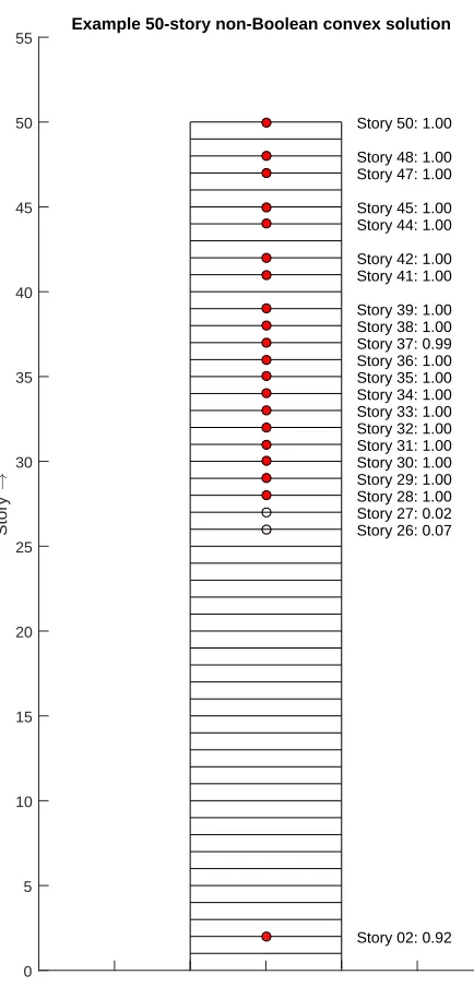
1.1 Organization of the thesis . . . 4 3.1 The resulting sensor locations after solving the convex optimization

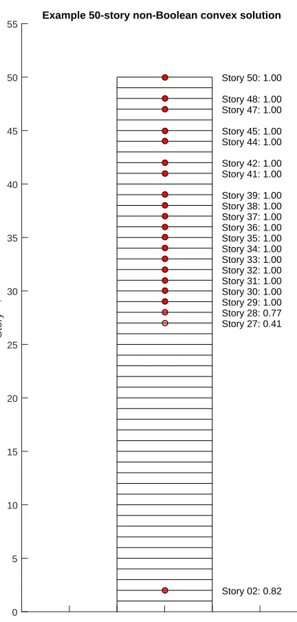
problem for a 50-story structure . . . 41 3.2 Another solution for the 50-story building but with different prior

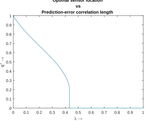
samples . . . 42 4.1 Optimal location of the second sensor as a function of the

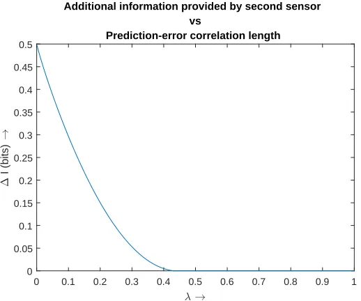
prediction-error correlation length scale (note that the first sensor is always at the free end of the cantilever beam) . . . 61 4.2 Additional bits of information from the optimally placed second

sen-sor plotted as a function of the correlation length scale . . . 62 5.1 The closed state-space trajectory of a double-well Duffing oscillator . 68 5.2 Period doubling bifurcation for forced, damped Duffing oscillator . . 69 5.3 Chaotic trajectory for a forced, damped Duffing oscillator . . . 69 5.4 Displacement trajectory plots of the data data from a linear oscillator

(blue) and a Duffing oscillator (red) . . . 73 5.5 Posterior component-wise marginal histograms for p(ζ|DL,ML) . . 76 5.6 Posterior component-wise marginal histograms for p(ζ|DL,MD) . . 77 5.7 Posterior component-wise marginal histograms for p(ζ|DD,ML) . . 77 5.8 Posterior component-wise marginal histograms for p(ζ|DD,MD) . . 78 5.9 Displacement trajectory plots for data from a linear oscillator (blue)

against the maximum a posteriori sample trajectory (red) from a linear oscillator model class . . . 79 5.10 Displacement trajectory plots for data from a linear oscillator (blue)

against the maximum a posteriori sample trajectory (red) from a Duffing oscillator model class . . . 79 5.11 Probability density function for the log-normal prior marginal for the

non-linear coefficient,α . . . 80 5.12 Displacement trajectory plots for data from a Duffing oscillator (blue)

LIST OF TABLES

Number Page

2.1 Simulation results for entropy-of-evidence . . . 20

2.2 Conditional entropy . . . 20

2.3 Mutual information estimate for a single DOF system . . . 21

2.4 Single degree-of-freedom example: Simulation parameters . . . 21

2.5 Two degree-of-freedom example: Simulation parameters . . . 22

2.6 Mutual information estimates for 2-DOF system . . . 22

3.1 Simulation results . . . 40

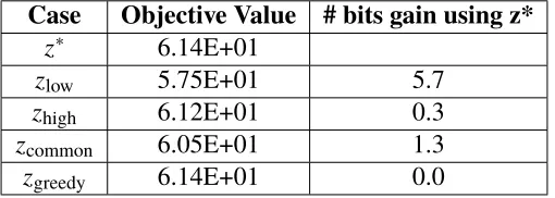
3.2 Description of various sensor configurations for comparative example 43 3.3 Comparison of information gain relative to optimal configuration . . 43

5.1 Specification of the data-generating parameters forML andMD . . . 71

5.2 Specification of priors forML andMD . . . 72

5.3 Data generating samples and MAP estimates for each scenario . . . . 81

5.4 AIMS parameters . . . 82

C h a p t e r 1

INTRODUCTION

An important goal of the field of structural monitoring is to use dynamic response data from an instrumented structure to perform system identification to quantify engineering quantities of interest such as substructure stiffness, as well as to make predictions about the future behavior of the structure. Response data is typically available in the form of acceleration records from ambient vibrations, vibration tests or seismic events. The parameters of a mechanical model that explains the behavior of a structure are typically sought. To this end, parametric system identification is used to quantify the values of parameters of the model that is assumed to govern the structure.

It is often not possible to postulate a true and exact model that explains the observa-tions and makes good predicobserva-tions. The primary reason for this is that the mechanical model used to describe the structure, however complex, will usually fail to account for every mechanical phenomenon, geometric and material detail correctly. In ad-dition, it is not clear how complex and detailed a model is appropriate, since a sufficiently adjustable model would always be able to explain the given observations at the cost of being able to make accurate predictions about future observations.

Given these limitations, in order to formulate a more meaningful system identi-fication problem, it is important to account for modeling uncertainties related to the prediction accuracy and the parameters associated with the mechanical model being considered. This is done by specifying a probability model for predicting the response based on the deterministic mechanical model of the structure and a proba-bility distribution over the uncertain parameters of the mechanical model, together known as a stochastic embedding of the parameterized deterministic model class, to form a stochastic model class [1].

The axioms of Bayesian probability form a foundation for performing plausible inference in a principled manner. Therefore, the data, together with the stochastic embedding, allow for the update of the distribution over the uncertain parameters of the model class.

instrumentation to be performed. Given that Bayesian inference will be done with the data, there is a problem to be addressed: the choice of optimal data-set to be collected for this inference.

This thesis will address the problem of optimal sensor location for Bayesian pa-rameteric system identification. For the purpose of illustration, consider a simple version of the sensor-selection problem of selecting a certain number of locations to be instrumented for structural monitoring, from a finite number of possibilities. For instance, one could imagine being budgeted with 20 sensors to be used to instru-ment a 50-story structure. In this situation, the number of possible configurations is roughly 47 trillion! The evaluation of any objective function for each such config-uration would be infeasible for even state-of-the-art computers available as of this writing.

There are several important factors to be considered when formulating an optimal sensor location problem:

• The measure of optimality used

• The type of data to be collected

• The choice of locations available for instrumentation

• Prior information about the structure to be instrumented

Each of these factors can have a significant impact on the solution to the problem and its solvability and will be addressed in this thesis.

The primary objective of this research is to introduce new methods for more effi-ciently solving existing formulations of the optimal sensor placement problem in the context of structural engineering. In addition, the assumptions made by contempo-rary formulations are relaxed to determine if the resulting more general framework is solvable.

1.1 General Overview

In the domain of earthquake engineering and structural dynamics, the optimal sensor location problem can be cast into a determinant maximization problem for an entropy-based objective function, if certain assumptions can be made about the stochastic model class. The first is that it should be globally identifiable under the selected data. In addition, it is assumed that a sufficiently large number of data points would be available so as to justify the use of the Laplace approximation to the posterior that would be obtained. Finally, a small parametric uncertainty is assumed. The optimization problem here is still one over all the possible sensor configurations available The use of genetic algorithms was proposed in [3] to obtain a sub-optimal and possibly near-optimal solution to the problem.

When such assumptions cannot be made for the problem under consideration, then the computational complexity of and theoretical insight into the problem deteriorates significantly. More advanced theoretical and computational formulations are needed to tackle such a problem.

So far, nothing has been said about what the possible sensor locations are or can be. In some problems, the possible sensor locations can be a pre-ordained constraint. For instance, consider the problem of selecting which stories of a building are to be instrumented based on a shear-building model. If the possible location in the floor for sensor placement in each story is fixed, then the possible sensor locations are already determined by the constraint of being only on floors.

In some problems, however, the possible sensor locations is a modeling choice. There are certain issues that can arise in this scenario. For instance, if there exists a highly informative “hotspot”, then the algorithm may have a tendency to cluster all available sensors near that location. This in turn is a result of a flaw in the modeling of the mutual informativeness of the sensors in such a configuration. This issue will be addressed here.

1.2 Contributions

Bayesian model updating

Mutual information-based optimal sensor placement

2-DOF system

Model class selection

Log-determinant formulation Combinatorial methods

Convex relaxation scheme Uniform shear _building Allowable sensor

locations Cantilever beam

MCMC and thermodynamic

integration

Figure 1.1: Organization of the thesis

configuration is.

In the process of attempting to computationally solve the fully general information-theoretic formulation, the evaluation of the Bayesian probabilistic quantity known as the evidence for the stochastic model class is necessary. A framework known as path sampling is shown to naturally arise out of a specific sampling algorithm. The model evidence thus calculated is used to perform model class selection using synthetic data from a linear oscillator versus one from a cubic non-linear, or Duffing, oscillator.

Finally, the current research draws on existing information-theoretic concepts to theoretically analyze and model certain specific situations that are encountered in the sensor selection problem, such as the effect of grid refinement on sensor selection, as well as sensor relocation.

1.3 Thesis outline

Figure 1.1 presents a flowchart depicting the thesis outline.

In Chapter 3 the problem is tackled for the situation in which simplifying assumptions about model class identifiablity and the suitability of applying Laplace’s approxi-mation to the posterior that is to be obtained, can be made. Methods developed in the field of convex optimization are incorporated into the solution method for the problem, in order to avoid a combinatorially large search for the optimal sensor configuration.

Chapter 4 discusses the effect of choices regarding the allowable sensor locations. Optimal sensor location on a continuous elastic bar is used as an example to illustrate the sensor placement on a continuum and to illustrate the relationship between the objective function and the mesh size. Finally, the effect of prediction-error correlation on sensor locations is discussed in the context of a cantilever beam.

Chapter 5 is a bit of a detour from the optimal sensor selection problem. The focus here is on demonstrating how a path sampling scheme arises naturally out of the AIMS Markov sampling algorithm for drawing posterior samples and can be used to estimate model evidence. The problem of model class selection between a linear and non-linear Duffing oscillator is tackled for data from either type of oscillator, to demonstrate consistency with existing interpretations of model evidence.

1.4 A note on terminology

References

[1] J. L. Beck, L. S. Katafygiotis, “Updating Models and Their Uncertainties. I: Bayesian Statistical Framework,”Journal of Engineering Mechanics, vol. 124, no. 4, pp. 455–461, Apr. 1998.

[2] J. Mitrani-Resier, S. Wu, J. L. Beck, “Virtual Inspector and its application to immediate pre-event and post-event earthquake loss and safety assessment of buildings,”Natural Hazards, vol. 81, no. 3, pp. 1861–1878, Apr. 2016.

C h a p t e r 2

MUTUAL INFORMATION-BASED OPTIMAL SENSOR

PLACEMENT

The Bayesian optimal sensor placement problem, in its full generality, seeks to maximize the mutual information between the uncertain parameters and the data to be collected for the purpose of performing Bayesian inference. This maximization is done over all possible sensor configurations for a given sensor budget.

Thus, in this chapter, a recap of the Bayesian model updating framework is first presented. The general expression for mutual information between prior and data for typical stochastic dynamical systems encountered in structural dynamics is presented next. Different interpretations of the mutual information objective are considered.

It is established that the computation of mutual information in the context of dynam-ical systems is computationally expensive. In order to make the problem tractable, certain simplifying assumptions are made to yield a more tractable objective func-tion. Later, Chapter 3 discusses an efficient convex relaxation scheme to determine possibly-optimal solution to the problem.

2.1 Introduction

The mutual information between two stochastic variables is an important quantity in experimental design for Bayesian system identification of stochastic dynamical systems. In this context, several possible interpretations of mutual information exist.

Prior information on the parameter values is expressed in terms of a prior distri-bution, p(θ|M). The stochastic forward model, typically denoted by p(y|θ,M), prescribes the probability of observing a particular data set given the parameters. The probability model class,M, is used to indicate a specific pairing of stochastic forward model and prior. The stochastic forward model with the actual data D substituted for y, when viewed simply as a function of the uncertain parameters,θ, is called the likelihood function.

the stochastic predictions can be denoted byp(y|M). This can be determined using the Total Probability Theorem, asp(y|M)=

∫

p(y|θ,M)p(θ|M)dθ

For a given data set, the parameter vector that maximizes the likelihood function is known as the maximum likelihood estimate (MLE), usually denoted by ˆθM LE. Similarly, the parameter vector that maximizes the posterior probability is known as the maximuma posteriori(MAP) estimate of the parameters, denoted usually by

ˆ θ_MAP.

2.2 Bayesian model updating

This section lays out the framework for Bayesian model updating for structural dynamics which forms the basis for the optimal sensor placement problem. The measured data on which inference is to be performed is assumed to be available in the form of dynamic test data in the time domain. It is assumed, here, that the complete system input can be determined given the parameters.

In a typical structural dynamics problem, one would have observed the acceleration, velocity or displacement time history at a certain number of locations. We shall assume, for the time being, that these locations are selected from among the degrees-of-freedom of a finite-element model that governs the structure.

Denote the uncertain system parameters byθs. These could correspond, for instance, to sub-structure stiffness, Rayleigh damping parameters or input ground acceleration amplitude. In general, they would depend on the mechanical model of the structure and the finite element approximation used to predict its response.

The prediction-error parameters are denoted by θe. When the prediction errors are modeled as Gaussian, with a stationary and isotropic co-variance matrix with diagnonal entriesσ2,θecould just be the scalar,σ. For an anisotropic model for the co-variance matrix without prediction error correlation between different locations, this could be a vector of variances corresponding to the diagonal entries of the co-variance matrix.

Denote byynthe stochastic prediction of the quantity to be observed at the time-point tn. Note that yn ∈ RNo, where No is the number of observed degrees-of-freedom out of a total of Nd degrees-of-freedom. The set of stochastic predictions for the observations over the whole duration of the measurement is denoted by y1:N.

n. δ ∈ {0,1}Nd is a Boolean vector that indicates the presence or absence of a

measurement sensor, so that the sum of entries ofδ equals the number of observed DOFs,No.

A sensor selection matrix, So(δ) ∈ RNo×Nd selects the components that are to be observed from the full stochastic prediction given by the sum of the deterministic prediction and noise terms.

The equation relating stochastic predictions to be observed, to the deterministic predictions, is, then:

yn =So(δ) (xn(θs)+n(θe)) (2.1)

In Equation (2.1),δ refers to a Boolean vector whose entries equal 1 when the re-sponse from a particular degree-of-freedom is observed, and 0 when not. The matrix So(δ)is a rectangular selection matrix and picks out those entries corresponding to

observed degrees of freedom.

LetM denote the probability model class. This includes the deterministic forward model with a stochastic embedding. The stochastic embedding, in turn, is specified by the stochastic forward model together with a prior distribution over the uncertain parameters. Our statistical modeling assumptions lead us to the following stochastic forward model:

p(y_1:N|θ,M)= N

Ö

n=₁

p(yn|θ,M) (2.2)

Bayes’ theorem can be used to perform the update as in Equation (2.3):

p(θ|y_1:N,M)=

p(y_1:N|θ,M)p(θ|M)

p(y_1:N|M)

(2.3)

The term in the denominator is called the evidence for the model class, M, under the data,DN and is given by the Total Probability Theorem in Equation (2.4):

p(y_1:N|M)=

∫

p(y_1:N|θ,M)p(θ|M)dθ (2.4)

This quantity will be dealt with in greater detail in Chapter 5 for the purposes of model selection.

The Prediction-Error Model

time and location, so that:

Ei,nj,m

=σ2δ

i jδmnwherei,n ∼ N(·|0, σ2)i.i.d. (2.5)

We then have an expression for the stochastic forward model:

p(y_1:N|θ,M)= N

Ö

n=₁

Nyn|So(δ)xn(θ), σ2

(2.6)

Using Bayes’ theorem, the distribution for the posterior, given the data is:

p(θ|y_1:N,M)=

p(y_1:N|θ,M)p(θ|M)

p(y_1:N|M)

= c−1_p(y

1:N|θ,M)p(θ|M) (2.7)

The evidence,c, for the model class in Equation (2.7) is treated simply as a normal-izing constant for the purpose of this section. In later sections such as in Chapters 5, it will be viewed as a function of the stochastic predictions as well as the model class.

The logarithm of the posterior is sometimes easier to work with. In the case of this example, we have:

logp(θ|y1:N,M) =−

N No

log 2πσ2

− 1

2σ2

N

Õ

n=₁

kyn−So(δ)xn(θs)k2+logp(θ|M) (2.8)

Note that when observations are actually made, then the collection of data at hand is denoted byDN = {yˆn}_nN₌

1or ˆy1:N.

2.3 Mutual information

The mutual information between two stochastic variables is a degree of measure about how much they imply about each others’ possible values. Formally, the mutual information between two continuous stochastic variables is defined as follows:

I(X;Z)= EX,Zlog

pX,Z(x,z)

pX(x)pZ(z)

(2.9)

The mutual information between two sets of stochastic variables is zero if and only if they are independent, since the joint density factors into the marginals. Additionally, if two stochastic variables are linearly correlated as in the case of a bi-variate Gaussian with a non-zero correlation coefficient, then the mutual information controls the correlation coefficient, ρ:

I(X;Z)= −1 2log

(₁− ρ2₎

The mutual information can be expressed as a difference of two entropies:

I(X;Z)= H(X) −H(X|Z) (2.11)

Equation (2.11) states that the mutual information is the difference in entropy of the marginal distribution for one variable and the conditional entropy. The expression is symmetric in either variable because of Bayes’ rule.

The conditional entropy is the entropy of one variable, conditioned on a partic-ular value of the other and averaged over that value according to its probability distribution. That is,

H(X|Z)=

∫

PZ(z)[H(X|Z = z)]dz (2.12)

The mutual information is always non-negative, since conditioning always reduces entropy or leaves it unchanged, on average.

In the Bayesian system identification setting, the mutual information quantity has several interpretations, that are discussed in the following sections.

Mutual information and Bayesian system identification

With the usual notation, the mutual information between the stochastic predictions for the observed data, y1:N, and the parameter vector,θ, is:

I(y_1:N(δ);θ)= Ey1:N(δ),θ|M

ln p

(y_1:N(δ), θ|M)

p(y_1:N(δ)|M)p(θ|M)

(2.13)

Equation (2.13) emphasizes the dependence of the stochastic prediction for the data, y_1:N(δ), on the sensor configuration, δ. This explicit dependence will be omitted

for convenience until a discussion of the optimal sensor location problem in Section 2.4.

Divergence from posterior to prior

I(y_1:N(δ), θ)= Ey1:N(δ),θ|M

ln p

(y_1:N(δ), θ|M)

p(y_1:N(δ)|M)p(θ|M)

(2.14)

= ∫ ∫ p(y_1:N(δ), θ|M)

ln p

(θ|y_1:N(δ),M)

p(θ|M)

dY dθ (2.15)

= ∫ ∫ p(θ|y_1:N(δ),M)p(y_1:N(δ)|M)

lnp

(θ|y_1:N(δ),M)

p(θ|M)

dY dθ

(2.16)

= Ey_1:N(δ)|MDK L[p(θ|y1:N(δ),M)||p(θ|M)] (2.17)

Here, the Kullback-Leibler divergence from one continuous probability distribution, P, to another,Q, specified by their probability density functionsp(x)_andq(x)_{, is:}

DK L(p(x)||q(x))=

∫ ∞

−∞

p(x)_logp(x)

q(x)dx (2.18)

The KL-divergence in this case can also be referred to as the relative entropy of P with respect toQ.

If one thinks of information maximization in the sensor placement framework, then maximizing this expected KL divergence would be equivalent to choosing the sensor configuration that has the largest expected reduction in entropy of the posterior distribution from the prior. Of all sensor configurations, the optimal one would result in the maximum reduction in entropy, on average, upon measuring the data.

Expression in terms of known quantities

The mutual information in a Bayesian system identification framework, usually involves only two specified distributions: the prior and the stochastic forward model. We can use Bayes’ theorem to express Equation (2.13) in terms of these distributions as:

I(y_1:N(δ);θ)= ∫ ∫

p(y_1:N(δ)|θ,M)p(θ|M)

log p

(y_1:N(δ)|θ,M)

p(y_1:N(δ)|M)

dy_1:N(δ)dθ

(2.19)

p(y_1:N(δ)|M) =

∫

p(y_1:N(δ)|θ,M)p(θ|M)dθ (2.20)

In principle, all these quantities should be calculable, givenp(θ)andp(y1:N(δ)|θ,M).

In practice, calculating these quantities turns out to be quite challenging. Section 2.6 addresses this issue.

2.4 Statement of the general problem

We propose to use the mutual information between the uncertain parameters and the data variable as the objective function to be maximized over sensor configuration. Consider the objective function:

maximize

δ I(y1:N(δ);θ)

subject to δi ∈ {0,1}, i =1, . . . ,Nd

and 1Tδ = No.

(2.21)

Equation (2.19) can be used for the objective function for the problem in (2.21). Recall thatδis a binaryNd-dimensional vector specifying the sensor configuration over the degrees of freedom in the system.

Log-determinant approximation

The mutual information criterion can be simplified to a more manageable log-determinant criterion when the following assumptions can be made about the prob-ability model class:

• The posterior distribution, upon collection of the data, is globally identifiable

• The Laplace approximation holds; that is, a sufficient of data points are measured so that the posterior is approximately Gaussian

Under these assumptions, the expression for mutual information may be simplified as follows. First, recognize the expression for mutual information as the KL-divergence from the posterior to the prior:

I(y_1:N(δ);θ)=Ey_1:N(δ),θ

log p

(θ|y_1:N(δ))

p(θ)

(2.22)

Begin by noting that the prior term is irrelevant in the sensor placement problem and may be discarded to yield the utility function,U(δ), as:

U(δ)=_Ey

Next, apply the Gaussian approximation to the posterior. That is,

p(θ|y_1:N(δ)) ≈ N(θ|θˆ(y_1:N),A−1(θˆ(y_1:N), δ)) (2.24)

Note that the precision matrix here is given by the Hessian of the logarithm of the stochastic forward model:

[A(θˆ(y_1:N), δ)]pq =−

∂2

logp(y1:N(δ)|θ)

∂θpθq (2.25)

The utility function becomes is now simply related to the entropy of this approxi-mately Gaussian posterior which may be expressed in terms of the log-determinant of its precision matrix as:

⇒U(δ)=−_Ey

1:N(δ)

constant− 1

2log detA

(θˆ(y_1:N), δ)

(2.26)

Finally, we assume that the expectation under the marginal distribution for the data equals that under the prior or nominal parameters, so that:

U(δ) ≈_constant+ 1

2Eθ

[_{log det}A(θ, δ)] _(2.27)

Hence, the mutual information utility function can be approximated by a Gaussian-like posterior entropy. Yet, there is still the matter of searching over possible sensor configurations. The convex optimization technique developed in Chapter 3 reduces the computational complexity of this search and provides expressions for the Hessian mentioned in Equation (2.26).

Comparison of two sensor configurations

Consider the difference in mutual information between two sensor configurations:

∆I₁₂ =∆ I(y_1:N(δ₂);θ) −I(y1:N(δ1)|θ)= H(y1:N(δ1)|θ) −H(y1:N(δ2)|θ) (2.28)

If the same approximations hold in either case, then we have:

∆I₁₂ = 1 2Eθ

[_{log det}A(θ, δ₂)] − 1

2Eθ

[_{log det}A(θ, δ₁)] _(2.29)

Now, note that the HessianA(θ, δ)consists of two block diagonal parts corresponding to the system parameters,θs and the single prediction error parameter,σ2. We may write:

Eθ[log detA(θ, δ)]=Eθs[log detB(θs, δ)]+Eσ2

For the same number of sensors, No, the scalar factor,C(σ2)= N N_2σ2o, cancels out in the difference.

We are left with the result:

∆I₁₂ = H(y_1:N(δ₁)|θ) −H(y_1:N(δ₂)|θ) (2.31)

= 1

2Eθs

[_{log det}B(θ_s, δ₂)] − 1

2Eθs

[_{log det}B(θ_s, δ₁)] _(2.32)

We can therefore compare the effect of sensor configuration on the difference in differential entropies of the posteriors that would result in the mean in each case.

2.5 Differences in mutual information

The mutual information between two stochastic variables is the mean increase in information of one variable upon learning the value of the other. This can be thought of as the mean gain in the number of bits of Shannon information, if the logarithm to the base 2 is used in the definition of entropy. (ref. CoverThomas)

In the expression above, the difference in values of the mutual information for two sensor configurations, therefore corresponds to the mean increase in bits of information gained relative to the prior for one configuration, δ1 versus the other,

δ₂.

2.6 Computing the mutual information

Recall that Equation (2.19) defines the mutual information that can in principle be solved. A piece of that equation is the evidence term which is given in equation (2.20).

To evaluate the mutual information, we split the expression from Eqn. (2.19) into two terms using the difference of the logarithms:

I(y_1:N(δ), θ)=

∫ ∫

p(y_1:N(δ)|θ,M)p(θ|M)[logp(y1:N(δ)|θ,M)

−_logp(y_1:N(δ)|M)]dy_1:N(δ)dθ (2.33)

=∫ p(θ|M)

∫

p(y_1:N(δ)|θ,M)logp(y1:N(δ)|θ,M)dy1:N(δ)dθ

−

∫

p(y_1:N(δ)|M)logp(y1:N(δ)|M)dy1:N(δ) (2.34)

⇒ I(y_1:N(δ), θ)= H(y_1:N(δ)) −H(y_1:N(δ)|θ) (2.35)

of a conditionally independent Gaussian stochastic forward model reduces to the expectation of a simple expression over the prediction-error uncertainty parameters only as will be seen in the examples that follow.

The entropy of the marginal distribution for the data prediction, on the other hand, is much harder to calculate in general, since an analytic expression for this marginal is usually unavailable. In addition, a single evaluation of the integrand involves one evaluation of evidence for the model class under that particular sample from the prediction for the data. As will be explored in Chapter 5, this is not a trivial task.

Methods to compute mutual information between low-dimensional variables exist, using samples from the joint distribution.

Monte Carlo approximation

Recall that mutual information can be decomposed into the difference of two en-tropies:

I(y_1:N(δ);θ)= H(y1:N(δ)) −H(y1:N(δ)|θ) (2.36)

Evaluation of the conditional entropy (the second term) is usually trivial in many situations such as when the prediction-errors are modeled as additive and inde-pendently Gaussian. This would typically involve calculating the expectation of the log-determinant of the co-variance matrix over the prediction-error uncertainty parameters.

The challenging computation is that of the entropy of evidence. A naive Monte Carlo approximation to this quantity is presented:

H(y_1:N(δ))=−

∫

p(y_1:N(δ))logp(y1:N(δ))y1:N(δ) (2.37)

≈ 1

Ns Ns

Õ

k=₁

logp(y1:N(δ) (k)₎

(2.38)

Here, y1:N(δ) (k)

is a sample from the joint distribution, p(y1:N(δ), θ). The variance

of a naive estimate of this might be quite high, since the data variable can be of a high dimension. However, this example is illustrative for the purpose of discussing the complexity of any sample-based estimate that uses roughly the same number of samples.

not straightforward, since again naive estimators tend to have high variance. To this end, a method of evaluating log-evidence is discussed in Chapter 5.

Example: Gaussian data with uncertain mean

The purpose of this example is to give insight into what the expression for mutual information may looks like. Consider a model classMG that specifies aNo-variate Gaussian stochastic forward model:

p(y_1:N(δ)|µ(θ),Σ(θ),MG)= N

Ö

n=₁

N(yn|µ(θ),Σ(θ)) (2.39)

= 1

(₂π)N No/2_|Σ(θ_)|N/2×

exp −1 2

N

Õ

n=₁

(yn−µ(θ))TΣ−1(θ)(yn−µ(θ))

!

(2.40)

It is also assumed that a prior model, p(θ|MG) is specified. In this case, the first term of Equation (2.35) is given by the expected entropy of a multivariate Gaussian distribution:

H(y_1:N|θ)= −Eθ

N

2 log

(₂πe)+ 1

2log det Σ(θ)

(2.41)

= −N No

2 log

(₂πe) − N

2Eθ

[_{log det}Σ(θ)] _(2.42)

On the other hand, the entropy of the distribution over the prediction of the data, or the entropy of the evidence density, is hard to calculate. This is because the marginal likelihood,p(y1:N|M), and its logarithm needs to be evaluated for every integration

point over y1:N. There is usually no closed-form expression to p(y1:N|M), except

perhaps when the predictions are linear in the parameters which in turn have a Gaussian prior, or when conjugate priors are employed. Again, these introduce restrictions on the class of models that may be employed and are usually not appro-priate modeling choices for dynamical systems. However, this example will look at the case where the prior for the mean parameter is chosen to be conjugate to the stochastic forward model.

To simplify this example further, assume that No = 1 so that the observations are modeled as univariate Gaussian data. Let only the mean be uncertain and have a Gaussian distribution, that isθ = µ∼ N(·|µ0, σ0). For simplicity, the

The resulting marginal likelihood is Gaussian:

p(y_1:N|MG)=

∫

p(y_1:N|µ)p(µ|µ0, σ0)dµ (2.43)

= ∫ 1

(₂πσ2)N/₂q

2πσ₀2 exp

"

− 1

2σ2

N

Õ

n=₁

(yn− µ)2−

(µ− µ₀)2

2σ₀2 #

dµ

(2.44)

= N y_1:N|µ01,Σ˜(σ0, σ)

(2.45)

where

|Σ˜(σ₀, σ)| = σ2N

1+ Nσ2

0

σ2

!

(2.46)

The mutual information between the prediction of the data and the uncertain mean parameter is therefore:

I(y_1:N;µ)=−N 2 log

(₂πeσ2₎+ N

2 log

(₂πe)+ 1

2log

|Σ˜(σ₀, σ)| _(2.47)

= N

2 log 1+ Nσ2

0

σ2

!

(2.48)

By inspection, Equation (2.48) tells us the following:

1. More observations,N, result in a higher mutual information

2. The data to be observed, y1:N, is more informative about the uncertain mean

parameter, µ, for a larger prior variance,σ₀2

3. For this contrived example, when the known prediction-error variance,σ2, is small, then this is an assertion that the observations are close to the predictions and therefore more informative

Example: Spring-mass oscillator

The simple case of a single degree-of-freedom dynamical system is considered next, to provide insight into mutual information calculations in more complicated cases. There is no analytical expression for the mutual information in this case.

Consider an undamped mechanical oscillator with uncertain natural frequency ω, with unit initial displacement and starting from rest. The governing equation is:

Ü

x+ω2_x=

0, withx(0)=1,xÛ(0)= 0 (2.49)

The solution to the displacement time history of this oscillator is:

x(t)=_cos(ωt) _(2.50)

We assume that data,y1:N = {yn}

N

n=₁, is obtained from points in time equally spaced

at∆t. The equation for the stochastic prediction is:

yn=cos(ωn∆t)+n (2.51)

As in the previous example, we assume the prediction-error to be stationary and Gaussian with uncertain varianceσ2, so that the stochastic forward model may be specified as:

p(y_1:N|ω, σ2,MO)= 1

(₂πσ2₎N/2 exp

"

− 1

2σ2

N

Õ

n=₁

(yn−cos(ωn∆t))2 #

(2.52)

Let the uncertain parameters be distributed according to a prior, as ω ∼ p(ω), σ2_{∼ p(}σ2_)andp(ω, σ2₎= _p(ω_)p(σ2_{). Then, the model evidence is given by:}

p(y_1:N|MO)=

∫ ∫

p(ω)p(σ2₎

(₂πσ2₎N/2exp

"

− 1

2σ2

N

Õ

n=₁

(yn−cos(ωn∆t))2 #

dωdσ2

(2.53)

Chapter 5 discusses the application of Asymptotically Independent Markov Sam-pling (AIMS) and path samSam-pling for the the purpose of evaluating model evidence, or integrals of the form:

p(y_1:N|M)=

∫

p(y_1:N|θ,M)p(θ|M)dθ (2.54)

In this example, the entropy-of-evidence term is determined as follows:

H(D) ≈ 1

Ns Ns

Õ

k=₁

logp(y_1:(k_N)|M) (2.55)

where

(y(k)

1:N, θ (k)_{) ∼}

p(y_1:N, θ|M)= p(y_1:N|θ,M)p(θ|M) (2.56)

Equations (2.55) and (2.56) specify that the entropy of evidence according to its Monte-Carlo approximations using samples from the predicted data variable. These samples come from the joint density. One sample from the joint is obtained by drawing a prior sample and running the stochastic forward model on it.

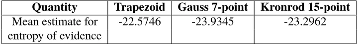
Each logarithmic term in the sum of Equation (2.55) is calculated using AIMS and path sampling. The sample average is an estimator for the mean. The standard devi-ation of the estimator of the mean is itself estimated using the standard reldevi-ationship between the sample and population variances.

Table 2.1: Simulation results for entropy-of-evidence

Quantity Trapezoid Gauss 7-point Kronrod 15-point

Mean estimate for -22.5746 -23.9345 -23.2962 entropy of evidence

The conditional entropy is evaluated much more easily, since it requires the expec-tation of the log variance under the prior:

H(y_1:N|θ)=

N

2 log 2π+ N

2 Eσ2

[_logσ2_]

(2.57)

In this case, we don’t even need use a Monte-Carlo estimate, since we have already specified that our prior standard deviation follows a log-uniform.

Table 2.2: Conditional entropy

Quantity Analytic Value

Conditional entropy -30.81061

Table 2.3: Mutual information estimate for a single DOF system

Quantity Mean

Mutual Information 8.2360

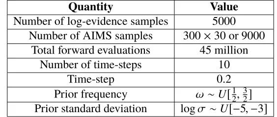
It should be noted that this evaluation is quite expensive. The simulation parameters for this example are listed in Table 2.4.

Table 2.4: Single degree-of-freedom example: Simulation parameters

Quantity Value

Number of log-evidence samples 5000 Number of AIMS samples 300×30 or 9000

Total forward evaluations 45 million

Number of time-steps 10

Time-step 0.2

Prior frequency ω ∼U[1₂, 3₂] Prior standard deviation logσ ∼U[−5,−3]

Example: Two-DOF unidentifiable system

Consider a 2-DOF system, consisting of two masses connected using two springs, with the end of one spring fixed. The equations of motion for this system are given by:

mxÜ(t)+

"

k₁+k₂ −k₂

−k₂ k₂ #

x(t)=_{0 (2.58)}

with

x(₀)=

( 1 1 )

(2.59)

We consider a unit mass, m = 1, for simplicity. This system can be diagonalized using a transformation matrixΦthat relates the modal co-ordinatesqjto the original onesxi. The resulting decoupled equations of motion have solutions:

qj(t)=(Φ₁j+Φ₂j)cos(ωjt) (2.60)

The solution to the original system, is therefore:

xi(t)=

Õ

j

This system has the peculiar property that the forward model output at the second degree-of-freedom can be matched for two very different stiffness configurations. The configurations[k1= k

∗

1,k2 = k ∗

2]and[k1 = 2k ∗

2,k2 = k ∗

1/2]result in identical

predictions for x2(t). On the other hand, the output x1(t)is defined uniquely.

For a specific prior, therefore, we expect to see a higher mutual information between the displacement at the first sensor location as opposed to the second. As in the previous example, the prediction-error parameter,σ, is uncertain. For this example, however, there are two uncertain system stiffness parameters, k1 and k2. The

stochastic forward model in either case is specified by:

p(y_1:N(δ = ei)|k₁,k₂, σ)= 1

(₂πσ2)N/₂exp

"

− 1

2σ2

N

Õ

n=₁

(yn−xi,n(k₁,k₂))2

#

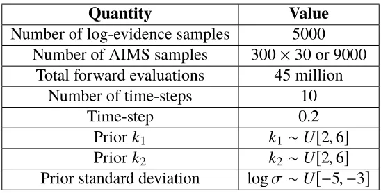
(2.62)

The parameters used for this simulation are listed in Table 2.5.

Table 2.5: Two degree-of-freedom example: Simulation parameters

Quantity Value

Number of log-evidence samples 5000 Number of AIMS samples 300×30 or 9000

Total forward evaluations 45 million

Number of time-steps 10

Time-step 0.2

Priork1 k1∼U[2,6]

Priork2 k2∼U[2,6]

Prior standard deviation logσ ∼U[−5,−3]

The mutual information is evaluated at both locations for each case and is presented in Table 2.6.

Table 2.6: Mutual information estimates for 2-DOF system

Location Mean

DOF1 4.7524 DOF2 5.0922

This warrants further analysis that is relegated to future work at this time, to verify that this is not an artefact of numerical computations.

Note that the number of time-steps was kept small and the measurement time-step fairly quite in order to keep in check the dimensionality of the data variable, while simultaneously being able to capture one whole period of oscillation for every frequency in the range of the prior.

2.7 Sensor rearrangement problem

The optimal sensor placement problem, in the absence of previous instrumentation of a structure, relies on a prior distribution over the parameters that has the maxi-mum entropic uncertainty for its model class, possibly with location and variance constraints.

When a structure has already been instrumented, however, a posterior distribution over the parameters is usually available after performing a Bayesian update. Here, we investigate whether or not a posterior could simply be used as the prior for a new optimal sensor placement problem.

Assumptions

To begin with, we assume that the same model class is chosen for the structure to be re-instrumented. Denote this model class byM.

Denote the data to be obtained from the new sensor configuration byY_N00(δ 0₎

. The data from the old configuration is, before performing the update, denoted byYN(δ). Then, we make the assumption that:

p(Y_N00(δ0),YN(δ)|θ,M)= p(Y_N00(δ0)|θ,M)p(YN(δ)|θ,M) (2.63)

This states that the new data is conditionally independent of the old data, given the parameter vector.

For convenience of notation, denoteYN(δ)byD1andY 0

N0(δ0)byD₂. For this problem,

we are given a realizationd1∼ D1. Also, conditioning onM is omitted.

In this notation, Equation (2.63) becomes:

p(D₂,D₁ =d₁|θ)= p(D₂|θ)p(D₁= d₁|θ) _(2.64)

Optimal placement for sensor reconfiguration

δ0

. We use the expected value of the KL-divergence from the updated prior to the pre-posterior given the as-yet-unmeasured data. That is:

U(δ0)=_ED

2|D1=d1[KL{p(θ|D2,D1= d1)||p(θ|D1 =d1)}] (2.65)

This may be further expressed as follows:

U(δ0)= _ED

2|D1=d1 ∫

p(θ|D₂,D₁= d₁)_log

p(θ|D₂,D₁= d₁)

p(θ|D₁ = d₁)

dθ

(2.66)

Conditional probability and Bayes’ theorem allows us to express this in terms of quantities that can be estimated numerically. Denote the logarithm term in Eqn. (2.66) by L(θ,D2,d1). Then, we have:

U(δ0)=

∫

p(D₂|D₁= d₁)p(θ|D₂,D₁= d₁)L(θ,D₂,d₁)dθdD₂ (2.67)

Using the conditional independence assumption of Eqn. (2.63), the logarithm term can be simplified:

L(θ,D₂,d₁)= _log

p(D₂|θ)p(D₁= d₁|θ)p(θ)p(D₁= d₁)

p(D₂|D₁= d₁)p(D₁= d₁)p(D₁= d₁|θ)p(θ)

⇒ L(θ,D₂,d₁)= _log

p(D₂|θ)

p(D₂|D₁= d₁)

(2.68)

Thus, upon simplifying the expression for the remaining terms, we get:

U(δ0)=

∫

p(D₂|θ)p(θ|D₁= d₁)_log

p(D₂|θ)

p(D₂|D₁ =d₁)

dθdD₂ (2.69)

The new problem, therefore requires evaluating the following entropy-like expres-sion:

H₂₁ =−

∫

p(D₂|D₁= d₁)_logp(D₂|D₁= d₁)dD₂ (2.70)

Further,

p(D₂|D₁ =d₁)=

∫

p(D₂|θ)p(θ|D₁= d₁)dθ _(2.71)

This implies that:

H₂₁ = logp(D1= d1) −

∫

p(D₂,D₁= d₁)

p(D₁= d₁) log{p(D2,D1= d1)} dD2 (2.72)

against θ in Equations (2.69) and (2.72) are against the posterior distribution over the parameters p(θ|D1 = d1), that have been updated using data from the first

deployment. Thus, the complexity of this problem is compounded by the fact that unlike the sensor location problem for which the prior distribution is easy to sample from, the sensor reconfiguration problem required drawing several sets of samples from the posterior distribution under the first set of data. An example problem is not attempted therefore, since reconfiguration problem, in the absence of any simplifying assumptions, is considerably more computationally expensive than the already costly sensor location problem.

References

C h a p t e r 3

EFFICIENT SOLUTION USING CONVEX RELAXATION

In the previous chapter, the Bayesian information-theoretic foundations of the op-timal sensor placement problem were laid out. Here, The entropy-based opop-timal sensor placement problem is formulated as in [1] and an efficient solution using con-vex optimization techniques is presented. Model identifiability is discussed and the Laplace approximation to the posterior in a Bayesian system identification problem is described.

3.1 Log-determinant formulation

This section expands on the derivation of the log-determinant formulation set up in Section 2.4. The Laplace approximation to the posterior together with addi-tional assumptions about the prediction-errors, allows for the development of a log-determinant entropy-based objective.

System Identifiability

The notion of identifiability is important to characterize the topography of the posterior distribution. The definition used here is in line with [2]. Essentially, the posterior distribution can either be globally identifiable, locally identifiable or unidentifiable as follows.

Denote by S(θ), the set of all admissible values of the parameter vector, θ. Also, let ˆθ correspond to the optimal parameters that maximize the likelihood function in Equation(2.6).

IfSopt(θ;DN), a subset of S(θ), is the set of all optimal models in the model class

M _{given data} D_{N, then a parameter}θ_{j is said to be} globally system identifiableif S_opt(θ_;D_N)_{contains only one optimal parameter, or else if for two different optimal}

parameter vectors ˆα(1)and ˆθ(2), the corresponding components of thej’th parameter are equal as ˆθ(j1) = θˆ

(₂)

j .

In general, a parameter is system identifiable if no two optimal parameters are arbitrarily close together. In other words, for ˆθ(_j1),θˆ(_j2) ∈ Sopt(θ;DN), there exists a

Finally, not that if a model is system identifiable but not globally so, then it is said to belocally system identifiable.

Laplace’s asymptotic approximation

When the system is globally identifiable, then we may expand the log-posterior about the most probable value to second order using a Taylor series to give us a Gaussian approximation to the posterior density:

p(θ|y_1:N,M) ≈ p(θˆ|y_1:N,M)exp

−1

2

(θ−θˆ)TAN(θˆ)(θ−θˆ)

(3.1)

The normalizing constant in front of the exponential can be determined by inspec-tion:

p(θ|y_1:N,M) ≈

p

detAN(θˆ) (2π)N No/2 exp

−1

2

(θ−θˆ)TAN(θˆ)(θ−θˆ)

(3.2)

The precision matrix of the multivariate Gaussian in Equation (3.1) is given by the Hessian of the logarithm of the posterior density, evaluated at the unique most-probable parameter vector. That is,

AN,i j(θ)= −

∂2_logp(θ_|y

1:N,M)

∂θi∂θj

(3.3)

It is to be borne in mind that the parameter vector and its associated derivatives can be partitioned into two parts - the system parameters and the prediction-error parameters:

AN(θs)=

"

BN(θs) 0

0 CN(σˆ) #

(3.4)

where

[BN(θs)]i j =

_∂2

logp(y1:N|[θs,σˆ],M) ∂θs,i∂θs,j

(3.5)

and

CN(σˆ)= ∂

2

logp(y1:N|[θs, σ],M)

∂σ∂σ

_σ=

ˆ σ

(3.6)

The posterior distribution of the system parameters only, with the prediction-error parameter marginalized out, can therefore be expressed independently as:

p(θs|y_1:N,M)=

p

detBN(θˆs) (₂π)N No/2 exp

−1

2

(θs−θˆs)TBN(θˆs)(θs−θˆs)

(3.7)

We now seek to provide an approximation to the diagonal block of the Hessian that corresponds to the system parameters,BN(θˆs), in terms of the sensitivity coefficients of the predictions with respect to the system parameters.

For fixed system parameters θs, the optimal (in the maximum-likelihood sense) prediction-error variance in terms of the data as:

ˆ σ2₍θ

s)= 1

N No N

Õ

n=₁

kyn−So(δ)xn(θs)k2

∆

= J(θ_s) _(3.8)

Equation (3.8) can be used to re-express the stochastic forward model at the optimal parameter:

p(y_1:N|θ = [θs,σˆ],M)= [2πeJ(θs)]−N No/2 (3.9)

We can evaluate the block diagonal terms of the Hessian corresponding to the system parameters by:

BN(θˆs)=

N No

2 ∂₂

J(θ_s)

∂θs∂θs

θs=θˆs

(3.10)

We expand the second-order derivative in Equation (3.10) using the expression for J(θ_s)_{from Equation (3.8):}

[BN(θˆs)]pq = 1

ˆ σ2

N

Õ

n=₁

" ∂xn

∂θs,p

SoSoT

∂x_nT ∂θs,q +

n

So

∂2_xn

∂θs,p∂θs,q

T#

(3.11)

With this assumption, the relevant portion of the Hessian matrix can be expressed in terms of the prediction sensitivity coefficients at the observed degrees of freedom. The resulting approximation for the second derivative is:

[BN(θˆs)]pq ≈ 1

ˆ σ2

N

Õ

n=₁

∂ xn

∂θs,p

SoSTo

∂xTn

∂θs,q

(3.12)

In addition, notice the dependence on the sensor configuration as SToSo = diag(δ). The expression in Equation (3.12) can therefore be transformed to a double-sum:

[BN(θˆs)]pq = 1

ˆ σ2

Nd

Õ

i=₁

δi N

Õ

n=₁

∂xn,i

∂θs,p

∂xT_n,i

∂θs,q (3.13)

Equation (3.13) is a linear sum of contributions of terms from each sensor location. For convenience of notation in the formulation of the optimal sensor placement problem, we use the following notation while discussing the matrix of the equation:

[BN(θˆs)]pq = 1

ˆ

σ2Qpq(δ)=

1 ˆ σ2

Nd

Õ

i=₁

δiQpq(ei) (3.14)

In Equation (3.14),

Qpq(ei)= N

Õ

n=₁

∂xn,i

∂θs,p

∂xT_n,i

∂θs,q (3.15)

Having developed an approximate expression for the posterior distribution over the system parameters, we are now in a position to discuss the optimal sensor location problem.

3.2 Entropy-based optimal sensor location

So far, we have discussed how data can be used to update uncertainties about our model. We now address the optimal sensor location problem. We begin by defining an objective function to be optimized with respect to sensor locations, that quantifies the posterior uncertainty that we expect in the parameters after measuring the data.

What is very convenient in the formulation of Section 2.2, is that the dependence on the data of the approximate posterior distribution over the uncertain parameters is only through the optimal parameters, ˆθ = θˆ(y1:N).

That is,

p(θ_s|y_1:N,M) = p(θs|θˆ(y1:N),M) (3.16)

The nominal values for the system parameters are used in place of the optimal parameters:

p(θs|θ₀,M)=

p

detBN(θs,₀) (₂π)N No/2 exp

−1

2

(θs−θs,₀)TBN(θ₀)(θs−θs,₀)

(3.17)

Since the designer is uncertain about the nominal values, a prior distribution,p(θ0),

is specified on the nominal parameters.

Equation (3.17) replaces the dependence of the posterior on the unavailable data with prior information that is already available in terms of the hyper-parameters, θ₀=[θs,₀, σ₀]. These hyper-parameters are either available in the form of structural

design information, or in the form of information obtained from preliminary tests.

Entropy-based objective

We are now in a position to specify an objective function to be optimized with respect to sensor location. Over all the possible sensor configurations, we would like to select the configuration that results in the lowest possible expected entropy of the pre-posterior, relative to the prior, upon arrival of the data.

∆H(δ)= H(θ_s|θ₀) −H(θ₀) _(3.18)

= E(θ_s,θ₀)[−logp(θs|θ₀)] −Eθ₀[−logp(θ0)] (3.19)

Only the conditional entropy term in Equation (3.18) depends on the value of the sensor configuration,δ. That is, we want to minimize w.r.tδ:

∆H(δ)= −1

2 ∫

log detQ(δ)p(θs,0)dθs,0+constant (3.20)

We now have an objective function to be optimized. The expression for Q(δ) comes from Equation (3.14). Denote the optimal sensor configuration byδ∗. Then, ignoring the irrelevant terms in Equation (3.20) we have:

δ∗ ₌

arg max

δ

∫

The entropy-based optimal sensor location problem is now fully specified in Equa-tion (3.21).

Complexity of the problem

Equation (3.21) specifies a combinatorial optimization problem. That is, the problem is of choosingNo sensor locations amongNd ones. Depending upon the problem, this could become prohibitively expensive. Each sensor configuration requires one evaluation of the expectation of the log-determinant of an expensive prediction. An example of a prohibitively expensive sensor placement problem is say one of selecting 20 locations from among 50 locations, to instrument: the number of possible combinations is about 47 trillion.

At this point, it is clear that a brute-force search for the optimal solution over all possible sensor configurations is not a wise approach. Instead, information obtained by evaluating different configurations should be used to guide the optimization process towards the optimal configuration.

It turns out that it is, in general, not possible to guarantee an optimal solution in a manner that does not require an exhaustive search. Heuristic methods such as genetic algorithms can produce an acceptable sub-optimal value if run for long enough. Incremental greedy algorithms are also guaranteed to produce a suboptimal value within(1−1/e)of the optimal [3], relative to the range from the least to the most optimal configuration.

The method developed in Section 3.3 along the lines of [4], applies a convex relaxation technique to provide a sub-optimal solution to the problem. An upper bound on the optimal value is automatically provided by the solution.

3.3 Convex relaxation of the combinatorial optimization problem

Here, a relaxed version of the optimization problem is set up and argued to be convex. The relevant partial derivatives of the objective function, that is, its gradient and its Hessian matrix are derived for the purpose of computing the solution. The final step involves replacing the expectation integral over the prior distribution on the uncertain parameters by its Monte Carlo approximation so that the problem may be solved by a generic convex solver. This is discussed in Section 3.3.

presented for specific scenarios.

Appendix A lists some of the useful matrix calculus identities used in evaluating the gradient of the objective. Appendix B contains detailed calculations relevant to the parametric gradient of the displacement predictions for the multistory structure example considered.

Combinatorial optimization problem

The original problem reflects the reality that a sensor must be present or absent at a degree of freedom. Thus, the optimization problem is over a boolean vector:

maximize

δ h(δ)

subject to δi ∈ {0,1}, i =1, . . . ,Nd

and 1Tδ = No.

(3.22)

The objective functionh(δ)corresponds to the gain in Shannon information associ-ated with a given sensor configuration,δ. It is given ([5]) by:

h(δ)=_Eθs[_{log det}Q(δ)] _(3.23)

The quantities in Equation 3.23 are summarized in Chapter 3. The negative sign simply converts the maximization problem to a minimization one in order to be consistent with the standard description of an optimization problem.

The practical difficulty in solving this problem is the fact that a naive exploration of all possibilities quickly becomes intractable over even moderate values of No

and Nd. For instance, the placement of 20 sensors in a 50 DOF structure would involve 50₂₀ ≈ 4.71×1013 evaluations of the objective function,h(δ). In order to overcome this difficulty, the original problem in Problem 3.22 is relaxed to allow the boolean vector δ to take values continuously between zero and one. The problem thus specified can be solved using convex optimization techniques that guarantee a relatively cheap and unique solution, as shown next.

Relaxed Problem statement

The original Boolean sensor placement vector, δ, is relaxed into a vector, z, in the hypercube[0,1]Nd, resulting in the relaxed optimization problem:

minimize

z f(z)

subject to −zi ≤ 0

zi ≤ 1, i =1, . . . ,Nd

and 1Tz= No.

(3.24)

Here, the objective is the continuous extension of the previous, converted to a minimization problem using a minus sign:

f(z)= −h(z)= −_Eθs[_{log det}Q(z)] _(3.25)

Note that this allows one to use continuous, rather than discrete, optimization packages to solve the problem.

Convex nature of the relaxed problem

Problem 3.24 describes a convex optimization problem. This is because the objec-tive function is a convex inz, and the equality and inequality constraints are affine, the log-determinant function in the objective is convex in z[4] and the expectation operator preserves the convexity of its argument. Thus, the problem has a unique global optimum. This can be determined computationally, as long as the objective can be computed at everyz.

For larger problems, it becomes necessary to supply the gradient and hessian of the objective with respect to z. This avoids expensive computations of their finite-difference counterparts. Fortunately, their expressions are tractable and, along with their Monte Carlo approximations, are described next.

Derivatives of the objective

∂f ∂zi

(z)=− ∂

∂zi

∫

log detQ(z, θs)p(θs)dθs (3.26)

=−

∫

∂log detQ ∂zi

p(θ_s)dθ_{s (interchange) (3.27)}

=−

∫

tr

Q−1∂Q

∂zi

p(θs)dθs (derivative of log-det) (3.28)

=−

∫

tr

Q−1₍z, θ

s)Q(ei, θs)

p(θ_s)dθ_{s (evaluation of partial) (3.29)}

= −

∫

Õ

Õ

Q−1

j k(z, θs)Qk j(e i_{, θ}

s)

ª ® ® ¬

p(θ_s)dθ_{s (trace of product) (3.30)}

= −

∫

Õ

Õ

Q−1

j k(z, θs)Qj k(e i_{, θ}

s)

ª ® ® ¬

p(θs)dθs (symmetry) (3.31)

= −_Eθs Q−1₍z, θ

s):Q(ei, θs)

(notation) (3.32)

The Hessian of the objective,

∂2_f

∂zp∂zq

(z)= − ∂

∂zq

Eθ

      Na

Õ

Õ

Q−1

j k(z, θs)Qk j(ep, θs)

      (3.33)

= −

_Eθ

      Na

Õ

Õ

∂Q−₁

j k(z, θs)

∂zq

Qk j(ep, θs)

      (interchanges) (3.34)

=

Eθ

Õ

Õ

Q−1∂Q

∂zq

Q−1

j k

(z, θs)Qj k(ep, θs)

     

(derivative of inverse)

(3.35)

=

E

tr

Q−1_(z)Q(eq_)Q−1_(z)Q(ep₎₍θ

s)

i

(derivative, trace)

(3.36)

=

Eθ

((Q−1_(z)Q(eq₎₎

:((Q−1(z)Q(ep))T)(θs)

(associativity, trace)

The expectation integral in the objective and its derivatives can be numerically approximated using stochastic simulations. These numerical approximations would be required for each constrained Newton step of the optimization scheme.

Numerical approximations

Given Nk samples θ(sk) distributed according to the prior p(θs) specified by the designer, the integrals in question may be approximated by their corresponding Monte Carlo estimates.

For the objective function,

f(z) ≈ 1

Nk

Nk

Õ

k=1

log detQ(z, θ(sk)) (3.38)

For the gradient of the objective,

∂f ∂zi

(z) ≈ − 1

Nk Nk

Õ

Õ

Õ

Q−1

j k(z, θ

(k)

s )Qj k(ei, θ

(k)

s ) (3.39)

Finally, for the hessian of the objective,

∂2_f

∂zp∂zq

(z) ≈ 1

Nk Nk

Õ

Õ

Õ

Q−1_Q(eq_)Q−1

j k

(z, θ(_sk))Q(ep, θ(sk))k j (3.40)

Some computational effort may be spared by noting that,

Q(z, θs)=

Nd

Õ

Õ

∂xl

∂θs

∂xl

∂θs T

(tn, θs) (3.41)

= Nd

Õ

l=1

zlQ(el, θs) (3.42)

Hence, stored values ofQ(ei, θs)may be used to determineQ(z, θs).

Solver for optimization