Gravity-driven flow of continuous thin liquid films on non-porous substrates with topography

This is a repository copy of

Gravity-driven flow of continuous thin liquid films on

non-porous substrates with topography

.

White Rose Research Online URL for this paper:

http://eprints.whiterose.ac.uk/1203/

Article:

Gaskell, P.H., Jimack, P.K., Sellier, M. et al. (2 more authors) (2004) Gravity-driven flow of

continuous thin liquid films on non-porous substrates with topography. Journal of Fluid

Mechanics, 509. pp. 253-280. ISSN 1469-7645

https://doi.org/10.1017/S0022112004009425

[email protected] https://eprints.whiterose.ac.uk/ Reuse

See Attached

Takedown

If you consider content in White Rose Research Online to be in breach of UK law, please notify us by

DOI: 10.1017/S0022112004009425 Printed in the United Kingdom

Gravity-driven flow of continuous thin liquid

films on non-porous substrates with topography

By P. H. G A S K E L L1, P. K. J I M A C K2, M. S E L L I E R1, H. M. T H O M P S O N1 A N D M. C. T. W I L S O N1

1_{School of Mechanical Engineering, University of Leeds, Leeds LS2 9JT, UK}

2_{School of Computing, University of Leeds, Leeds LS2 9JT, UK}

(Received11 August 2003 and in revised form 23 January 2004)

A range of two- and three-dimensional problems is explored featuring the gravity-driven flow of a continuous thin liquid film over a non-porous inclined flat surface containing well-defined topography. These are analysed principally within the frame-work of the lubrication approximation, where accurate numerical solution of the governing nonlinear equations is achieved using an efficient multigrid solver.

Results for flow over one-dimensional steep-sided topographies are shown to be in very good agreement with previously reported data. The accuracy of the lubrication approximation in the context of such topographies is assessed and quantified by comparison with finite element solutions of the full Navier–Stokes equations, and results support the consensus that lubrication theory provides an accurate description of these flows even when its inherent assumptions are not strictly satisfied. The Navier– Stokes solutions also illustrate the effect of inertia on the capillary ridge/trough and the two-dimensional flow structures caused by steep topography.

Solutions obtained for flow over localized topography are shown to be in excellent agreement with the recent experimental results of Decr´e & Baret (2003) for the motion of thin water films over finite trenches. The spread of the ‘bow wave’, as measured by the positions of spanwise local extrema in free-surface height, is shown to be well-represented both upstream and downstream of the topography by an inverse hyperbolic cosine function.

An explanation, in terms of local flow rate, is given for the presence of the ‘downstream surge’ following square trenches, and its evolution as trench aspect ratio is increased is discussed. Unlike the upstream capillary ridge, this feature cannot be completely suppressed by increasing the normal component of gravity. The linearity of free-surface response to topographies is explored by superposition of the free surfaces corresponding to two ‘equal-but-opposite’ topographies. Results confirm the findings of Decr´e & Baret (2003) that, under the conditions considered, the responses behave in a near-linear fashion.

1. Introduction

containing topographical features. The latter may be regular and desired (patterned) or unwanted (a random scratch or speck of dust). Similarly, many manufactured products, particularly in the electronics sector (micro-devices, sensors, printed circuits, displays, etc.), usually involve the successive deposition of several thin liquid layers, combined with photolithography at each stage. Therefore, in the subsequent formation of the desired component/surface each layer is influenced by the one deposited and cured previously which, if non-uniform, presents the current wet layer with a surface that may lead to variations in coating thickness or even instabilities. Whatever the situation, increasing demands concerning quality and finish have promoted the need for better understanding of the mechanisms leading to free-surface non-uniformities and how to control/suppress the occurrence of their attendant undesirable defects.

Most previous investigations have concerned thin film flows over two-dimensional topography. Important early examples are the combined theoretical and experimental studies of Stillwagon & Larson (1987, 1988, 1990) and Pritchard, Scott & Tavener (1992) who considered radial outflow during spin coating and gravity-driven flow down an inclined plane, respectively. Both sets of authors demonstrated lubrication theory to be surprisingly accurate for modelling purposes even for cases where it is not strictly valid, as for the flow over shallow trenches. Stillwagon & Larson (1990) are also credited with being the first to obtain a one-dimensional analytical expression for the standing capillary wave at the leading edge of a trench and its associated downstream exponential decay. Of note also is the work of Roy & Schwartz (1997) which extended the one-dimensional lubrication approach to general curved substrates with topography by expressing the problem in curvilinear coordinates. Following a different tack, Decr´e, Fernandez-Parent & Lammers (1999) revisited the flow studied by Stillwagon & Larson (1990) and presented a Green’s function formulation to the problem. The second-order term contained therein has the effect of locating the capillary ridge further upstream of the topography, the deeper the trench becomes.

More recently, Kalliadasis, Bielarz & Homsy (2000) returned to the problem of the flow over a trench under the action of an external body force, solving the assumed governing one-dimensional long-wavelength, or lubrication, approximation numeri-cally as a means of analysing further the case of trench depths comparable with, or larger than, the associated unperturbed film thickness. Their results show that deep trenches produce an asymmetry, with the step-down leading to a comparatively more pronounced capillary ridge than the step-up. They also explored the effect of gravity, showing that it could result in the disappearance of capillary ridges. The stability of the latter was considered in a subsequent article, Kalliadisis & Homsy (2001). The picture was essentially completed by Mazouchi & Homsy (2001) who solved the corres-ponding Stokes problem numerically using a boundary element method and compared the results with those obtained using lubrication theory. They demonstrated the importance of the capillary number,Ca, and in particular that increasing it leads to a diminution or flattening of the capillary ridge, with the free-surface correspondingly conforming more to the topography of the substrate.

is, a standing ‘bow wave’ capillary ridge upstream of the particle together with an exponentially decaying, ‘horseshoe’-shaped capillary wake downstream. Other work of note is that of Peurrung & Graves (1991, 1993) for the case of spin coating over topography. Their experimental and numerical results are found to be in qualitative agreement, but for shallow topographies of the order of 1µm deep the absolute accuracy of their experimental data is questionable. Hayes, O’Brien & Lammers (2000) formulated a Green’s function for the linearized two-dimensional lubrication equations for the flow over a shallow topography which allowed the surface responses to arbitrary finite topographies to be calculated.

The motivation for the present work is provided by the recently reported painstaking quantitative experimental results of Decr´e & Baret (2003) for the case of gravity-driven flow of thin water films over topography. Building on earlier work (Mess´e & Decr´e 1997; Decr´e et al. 1998, 1999; Luc´ea & Decr´e 1999), they used phase-stepped interferometry to obtain detailed free-surface maps for thin films of water flowing down an inclined plate containing a range of topographies. In all cases, results compare well with those of earlier studies and, in the case of flow over three-dimensional topography, with the results of Hayes et al. (2000) for the linearized problem. A consequence of the latter is that linear superposition may be used to construct an approximate free-surface response to a complex topography from knowledge of the responses to regular elementary topographies.

2. Problem specification and mathematical formulation

Flow of a continuous film of liquid, fluxQ0, over a plane surface (streamwise extent LP and span widthWP) inclined at an angleθ to the horizontal arises as part of many manufacturing processes, with the case of flow over a smooth homogeneous surface now recognized as a classical problem in fluid mechanics. If the liquid is assumed Newtonian and incompressible, with constant density ρ, viscosity µ and surface tension σ, its steady motion in the general sense is governed by the Navier–Stokes and continuity equations:

ρU· ∇_{U =−}∇_P+µ∇2_{U+ρg, (2.1)}

∇ ·_{U = 0, (2.2)}

where U= (U, V , W) and P are the fluid velocity and pressure respectively and

g= (gsinθ,0,₋gcosθ) is the acceleration due to gravity.

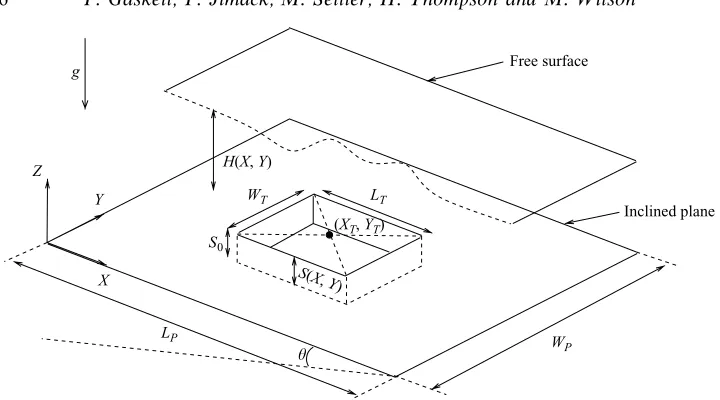
In the problems of interest here, the inclined substrate contains well-defined topo-graphical features of amplitude S0 and form S(X, Y), with streamwise extent LT and span width WT, centred at (XT, YT). These features may completely span the domain (in which case WT=WP and LT≪LP, leading to two-dimensional flow), or be localized (i.e. WT≪WP andLT≪LP, giving three-dimensional flow). The former problem reduces conveniently to solving for the flow in a streamwise cross-section only, provided WP is sufficiently large for end effects to be negligible. In both cases the topography may be a protrusion (S0>0) or a depression (S0<0) as sketched in figure 1. These are often referred to as ‘peaks’ and ‘trenches’ respectively.

2.1. Full-width topography

g

X Y

Free surface

Inclined plane

0 S

W_P

Z H(X, Y)

θ S(X, Y₎

WT LT

LP

(XT, YT)

Figure 1.Schematic diagram of a three-dimensional thin film flowing over a substrate inclined at angle θ to the horizontal, showing the coordinate system and parameters defining the topography.

analysis is fundamental to determining the validity of the lubrication approximation as a suitable means of solving three-dimensional flow over localized steep-sided topography.

Following Aksel (2000), an appropriate length scale for non-dimensionalization purposes is the undisturbed fully developed film thickness:

H0=

3µQ0 ρgsinθ

1/3

, (2.3)

while the characteristic velocity U0 is taken to be the surface velocity of the fully developed film:

U0 = 3Q0 2H0

. (2.4)

Implicit in the choice of scales (2.3) and (2.4) is the assumption that θ= 0, i.e. the substrate is never horizontal. Scaling velocities, axial coordinates and pressure byU0, H0 and µU0/H0 respectively, and noting the absence of any Y dependence, allows equations (2.1) and (2.2) to be rewritten in the form:

Reu· ∇_u=∇ ·τ +Stgˆ, (2.5)

∇ ·_{u= 0, (2.6)}

where u= (u, w) is the non-dimensional velocity in the dimensionless (x, z)-plane, Re=ρU0H0/µ= 3ρQ0/2µis the Reynolds number,τ=−pI+∇u+ (∇u)T is the non-dimensional Newtonian stress tensor, and St=ρgH₀2/µU0= 2/sinθ is the Stokes number.

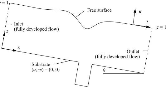
The boundary conditions which close the problem are shown in figure 2. On the substrate the no-slip condition u=w= 0 is applied and at the inflow and outflow planes a fully developed velocity profile is assumed:

u= 1

2Stsinθ(2z−z 2₎

Substrate (u, w) = (0, 0) x

z z = 1

z = 1 Free surface

Inlet

(fully developed flow)

Outlet (fully developed flow)

θ

n

t

Figure 2. Schematic diagram of flow over a one-dimensional (spanwise) topography.

On the free surface the usual stress and kinematic conditions,

n·τ = 1

Ca dt

ds and n·u= 0, (2.8)

are imposed (where nand t are the unit normal and tangent to the free surface, and s is arclength along it). Using scales (2.3) and (2.4), the capillary number is given by

Ca=µU0/σ =

1 2

9µ2ρgsinθ σ3

1/3

Q2₀/3. (2.9)

Finally, at each end of the domain the dimensionless film thickness is set equal to one, i.e. the fully developed thickness.

2.2. Localized topography

Three-dimensional steady flow over localized topography is analysed using a lubrica-tion approximalubrica-tion. The problem to be solved results from a long-wave expansion of equations (2.1) and (2.2) under the assumption that ǫ=H0/L0 is small, where L0 is the characteristic in-plane length scale. Retaining U0 and H0 as defined above, the resultant lubrication equations for the film thickness H(X, Y) and pressure field P(X, Y) are formulated in terms of the following non-dimensional variables:

h(x, y) = H(X, Y) H0

, s(x, y) = S(X, Y) H0

, (x, y) = (X, Y) L0

,

z= Z H0

, p(x, y) = 2P(X, Y) ρgL0sinθ

, (u, v, w) =

U U0

, V U0

, W ǫU0

.

Note that the surface of the substrate is given in terms of the topography function s(x, y) so that the fluid film lies between z=s and z=h+s. Introducing the above scalings into the governing equations and neglecting termsO(ǫ2_{) yields:}

∂2u ∂z2 =

∂p

∂x −2, (2.10a)

∂2v ∂z2 =

∂p

∂y, (2.10b)

∂p

Equations (2.10a, b) are solved subject to the no-slip condition (u, v) = (0,0) on the substrate,z=s, and zero tangential stress at the film surface, i.e.

∂u ∂z =

∂v

∂z = 0 atz=h+s. (2.11)

Integrating equations (2.10a, b) twice with respect to z over the film thickness z_∈[s, h+s] subject to the above boundary conditions yields

u=

∂p ∂x −2

(z₋s)1

2(z−s)−h

, (2.12a)

v=

∂p ∂y

(z₋s)₁

2(z−s)−h

. (2.12b)

That mass is conserved throughout the solution domain gives rise to the constraint

∇ · _{Q= 0, (2.13)}

where Q=h+s s (u, v)

T_{dz. Integrating equations (2.12a, b) to form Qand substituting} into equation (2.13) yields the following steady-state lubrication equation for h in terms of the pressure field,p:

0 = ∂ ∂x h3 3 ∂p ∂x −2

+ ∂ ∂y h3 3 ∂p ∂y . (2.14)

The pressure field throughout the film is obtained by integrating equation (2.10c) with respect toz, with the constant of integration (setting the pressure datum to zero) determined by

−ǫ

3

Ca∇

2₍

h+s) on z=h+s, (2.15)

hence,

p=₋ǫ 3

Ca∇

2₍

h+s) + 2ǫ(h+s₋z) cotθ. (2.16) Note that thez-dependence in equation (2.16) due to the 2ǫzcotθ term does not have any influence on the film thickness hsince its partial derivative with respect to both x andy is zero. Accordingly, this term is omitted in what follows.

So far, the choice of length scaleL0 has been arbitrary, but choosing it to be equal to the capillary length,Lc,

L0=Lc=

σ H0 3ρgsinθ

1/3

= H0

(6Ca)1/3, (2.17)

enables the pressure, equation (2.16), to be rewritten as

p=₋6_∇2(h+s) + 2√36N(h+s), (2.18) i.e. in terms of the parameterN=Ca1/3_cot

θ, which measures the relative importance of the normal component of gravity (Bertozzi & Brenner 1997). Note that ifN_≪1 the normal component of gravity becomes negligible (Troian et al. 1989), and equation (2.18) becomes parameter-free in the sense that the behaviour of the thin film will depend only on the topographic features.

later it is convenient to define a coordinate system (x∗, y∗) whose origin is at the centre, (xt, yt), of the topography. With (x∗, y∗) = (x−xt, y−yt) such thath∗(x∗, y∗) = [h(x∗, y∗) +s(x∗, y∗)₋1]/s0,s(x, y) is given by

s(x, y) = s0 b0

tan−1

x∗₋wt/2

γ wt

+ tan−1

−x∗₋wt/2

γ wt

×

tan−1

y∗₋lt/2

γ wt

+ tan−1

−y∗₋lt/2

γ wt

, (2.19)

where γ is an adjustable parameter which defines the steepness of the topography, A=wt/ lt is the aspect ratio of the topography, and

b0 = 4 tan−1

1 2γ

tan−1

A 2γ

. (2.20)

The following boundary conditions, resulting from the assumption that the flow is fully developed both upstream and downstream:

h(0, y) = 1, ∂h ∂x _x =0

= 0, ∂h ∂x _x =1 = ∂p ∂x _x =1

= 0, (2.21)

together with the requirement of zero flux at the boundaries in the spanwise direction:

∂p ∂y y=0 = ∂p ∂y y=1 = ∂h ∂y y=0 = ∂h ∂y y=1

= 0, (2.22)

effectively close the problem.

3. Method of solution

3.1. Finite element formulation

The finite element (FE) method used to solve equations (2.5) and (2.6) in two dimen-sions, subject to the given boundary conditions, employs a popular Bubnov–Galerkin weighted residual formulation that has been applied successfully to a wide variety of incompressible flow problems. Since it has been described in detail elsewhere, see for example Christodoulou, Kistler & Schunk (1997), only a very brief overview is given here. The free surface of the film is parametrized by a ‘spinal’ algebraic mesh generation algorithm, Kistler & Scriven (1983), and the two-dimensional flow domain is tessellated using V6/P3 triangular elements (Gaskell et al.1995; Summers

et al. 2004) giving a piecewise quadratic velocity field and a piecewise linear pressure

field. Note also that topographies in the FE analysis are completely sharp, i.e. corners are perfect right angles, since there is no need to use the approximating arctangent functions as in equations (2.19) and (2.20). The free-surface kinematic condition

n·_{u= 0 is used to determine the free-surface location while the free-surface stress}

conditions enter the FE formulation via a boundary integral arising in the weak form of equation (2.5) – see Kistler & Scriven (1983) for further details.

meshes was less than 0.05% when measured in the way described in_§4.1. For each mesh the locations of the inflow and outflow boundaries were checked to confirm that they had a negligible effect on the solution. This is particularly important upstream, because the free surface always features a wave which decays with distance upstream from the topography. Hence the inflow boundary should be located where the amplitude of the wave is sufficiently small so that the imposition of h= 1 does not unduly distort the free surface.

For all the parameter values used in the simulations involving full-width topo-graphies, it was found (by considering a much larger domain) that the amplitude of the upstream capillary wave reduces toO(10−7_{) at a distance of 30L}

c upstream of the topography. Downstream of the topography the free surface relaxes monotonically to the fully developed film thickness such that after a distance of 15Lc the free-surface height is within 10−7 _{of the asymptotic height. These positions were therefore taken} to be sufficient to guarantee the accuracy of the solution of the whole domain. The first two wavelengths of the capillary wave lie typically within 15Lc or 20Lc of the topography, and so this could be considered as a minimum domain size. Note that localized topographies produce effects which are felt further downstream than in the full-width case, and therefore a larger domain size is needed to produce the results in _§4.2. In the step-up/-down and trench problems domain tessellations comprising respectively 5650 and 5900 elements were utilized; in each case 701 spines were used to parametrize the free-surface position.

3.2. Finite difference formulation

Although using a lubrication approximation to model the flow over localized topo-graphy effectively reduces the dimensionality of the problem by one, solution of the resultant equations still poses a considerable computational challenge due to the stiffness introduced via the surface tension. Accordingly, the recently derived accurate and robust Full Approximation Storage (FAS) multigrid approach of Gaskell et al. (2004) is employed since its fully implicit nature has already been demonstrated to offer increased efficiency, particularly when fine grid resolution is essential. In addition, rather than substituting equations (2.16) or (2.18) for the pressure into equation (2.14) to yield a fourth-order partial differential equation for the film thicknessh, these two coupled equations are retained and solved in their present form since they are simpler to incorporate into the FAS multigrid solution strategy.

Equations (2.14) and (2.18) are discretized using second-order-accurate central differences on a square computational domain so that (x, y)_∈Ω= (0,1)_×(0,1). The mesh is uniformly structured with (2k_{+ 1) nodes in each direction. Unless stated} otherwise,k takes the value 10, yielding solutions on a 1025_×1025 mesh containing in excess of one million grid points. The corresponding coupled algebraic analogues are:

0 = 1

2 pi+1,j 1 3h

3

|i+1/2,j +pi−1,j₃1h3|i−1/2,j−pi,j ₁

3h 3

|i+1/2,j +1₃h3|i−1/2,j

−21 3h

3

|i+1/2,j −1₃h3|i−1/2,j

+pi,j+11₃h3|i,j+1/2 +pi,j−11₃h3|i,j−1/2−pi,j

1 3h

3

|i,j+1/2+ 1₃h3|i,j−1/2

, (3.1)

pi,j + 6

2[(hi+1,j+si+1,j) + (hi−1,j+si−1,j) + (hi,j+1+si,j+1) + (hi,j−1+si,j−1)−4(hi,j +si,j)]−2

3

√

for each (i, j) in the computational domain, where = 2−k _{is the spatial increment.} The terms 1

3h 3_|

i±1/2,j±1/2, sometimes referred to as prefactors, result from linear interpolation between the neighbouring vertices,

1 3h

3_|

i+1/2,j = 1₂ 1

3h 3 i+1,j +

1 3h

3 i,j

, (3.3)

with analogous expressions for the other prefactors.

Boundary conditions (2.21) and (2.22) are eliminated from equations (3.1) and (3.2), as opposed to introducing ghost nodes at the boundary, since this is found to reduce the bandwidth of the matrix to be inverted. A computational domain extending over 100 capillary lengths was found to be sufficient to ensure accurate solutions. The resulting system of nonlinear algebraic equations is solved for hi,j and pi,j using an FAS multigrid algorithm with V-cycling (Brandt 1977). In brief, Gauss–Seidel relaxation is employed with a ‘red-black’ ordering of the nodes. At each level, down to the coarsest, a fixed number of sweeps is applied to a linearized form of the equations in order to update previous estimates of the solution on that grid. At the coarsest level, the system of algebraic equations is solved exactly using Newton iteration. A further series of Gauss–Seidel post-smooths is then applied on successively finer grids in order to complete the V-cycle. The recent comprehensive article by Gaskell

et al. (2004) gives a more detailed explanation of the methodology.

The only other feature of importance to note is that the problems of interest are steady state. Obtaining such solutions is a little more demanding than in the case of transient behaviour where a small fixed number of V-cycles is sufficient to reduce residuals by a constant factor for successive time steps (Gaskell et al. 2004). Accordingly, the nonlinearity in the discrete algebraic system is found to be more severe than experienced in the case of implicit time stepping, and the quality of the initial guess is much poorer, which in turn means that typically more V-cycles are required. Hence, it was found that a total of about 15 V-cycles is necessary to reduce residuals to within that of the discretization error, 10−6_{, on the prescribed} finest 1025_×1025 mesh level. However, even with such a necessary large number of V-cycles the multigrid algorithm proves to be a robust and efficient scheme, with its rate of convergence independent of the final specified finest mesh. As a check, the problems considered in _§4.1 were also solved using the time adaptive scheme described in Gaskell et al.(2004) starting from an initial condition of a flat free-surface profile. In all cases these solutions evolved to correspond exactly to their steady-state counterparts, as shown in figure 3. Unsurprisingly, although the transient method of solution requires significantly fewer V-cycles per iteration the overall time required to reach steady state is significantly more due to controlling the time step in order to achieve accurate solutions to a specified temporal error tolerance.

4. Results and discussion

4.1. Flow over full-width spanwise topographies

–30 –20 –10 0 10 20 30 x*

–0.8 –0.6 –0.4 –0.2 0 0.2

h*

t = 0.1

0.15 0.2 2.5 0.3 0.4 0.5 Steady state

Figure 3. Free-surface profile for flow over a one-dimensional trench, demonstrating the progression of the transient solution towards the solution of the steady-state equation.

–20 0 20 40 60

X/H0 –1.0

–0.5 0.0 0.5 1.0 1.5

h

Ca = 0.005 Ca = 0.05

Mazouchi & Homsy (2001) Present work with Re = 0 Present work with Re = 10 Topography

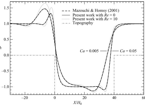
Figure 4.Comparison of film profiles calculated by the FE method with the boundary element profiles of Mazouchi & Homsy (2001). The trench has depth 2H0 and width 40H0. Note that for ease of comparison with Mazouchi & Homsy, their axis scales are used. Hence x and h are both scaled byH0.

Mazouchi & Homsy (2001). It is clear from the figure that excellent agreement is achieved between the FE and BE predictions when Re= 0.

Also shown in the figure are two FE-generated profiles indicating the effect that increasingReto 10 has on the free-surface shape. IncreasingReincreases the velocity of the fluid travelling down the inclined plane, and this results in a shortening of the wavelength of the capillary wave propagated upstream from each step face. The first peak (trough) of each wave is also pushed towards its step face by the increased inertia, and the amplitude of each wave is noticeably increased. This enlargement of the capillary ridge provides an increased capillary pressure which helps to decelerate the fluid in the x-direction and deflect the film round the corner of the step. Similar effects have been observed in slide coating (Christodoulou & Scriven 1989) and also in the flexible-walled channel flow studied by Heil (2000), where the shape of the flexible wall containing the flow exhibits a behaviour comparable to that of the free surface in figure 4 in response to an increase in fluid inertia.

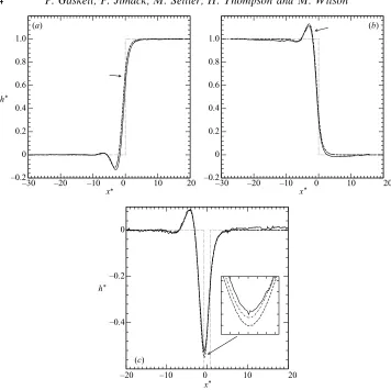
Decr´e & Baret’s (2003) recent experimental study of thin water films flowing down an inclined plane with topographies is another valuable source of data to compare to numerical predictions. Figure 5 presents a comparison of FE and lubrication solutions for free-surface profiles to those found experimentally by Decr´e & Baret (2003) for the cases of flow over a small one-dimensional step-down, a step-up and a trench. The Reynolds number was 2.45 for the steps and 2.84 for the trench. Note that in this and subsequent comparisons in this section, liquid properties are taken asµ= 0.001 Pa s,ρ= 1000 kg m−3 _{andσ= 0.07 N m}−1_{, and the inclination angle is set} toθ= 30◦_{. In all three cases the FE and lubrication solutions are seen to be practically}

indistinguishable (see below), to agree well with experiment and to reproduce accurately the main features of the film thickness profiles, such as the characteristic free-surface trough and capillary ridge just upstream of the step topographies and the free-surface depression characteristic of flow over the trench.

Since the FE solutions do not have the inherent limitations of those based on lub-rication theory, they can be used to assess the accuracy of the long-wave approxima-tion in relaapproxima-tion to flow over topography. Figures 6 and 7 show contours which quantify the discrepancy between the two types of solution as step height and flow rate are varied in flow over both step-up and step-down topography. The difference is defined as the maximum distance between the predicted lubrication film thickness and its Navier–Stokes counterpart, measured normal to the lubrication profile. This measure is preferred to one based on an r.m.s. distance since both profiles satisfy the same boundary conditions far upstream and downstream of the topography so that the latter measure would be unduly influenced by the long asymptotic regions of the domain where the two profiles are practically indistinguishable. Note that in making the comparisons, the asymptotic film thickness,H0, is used as the length scale in both the x- and z-directions. The contours therefore give the error between lubrication theory and finite element analysis as a percentage ofH0. For both up and step-down topography the position of the maximum difference between corresponding profiles is near the top of the steeply sloping part of the profile, as indicated by the arrows in figures 5(a) and 5(b). The difference in the predictions of the height (depth) of the capillary ridge (trough) is typically much smaller, roughly 1/4 of the maximum difference. Note that the vertical scales in figures 6 and 7 indicate both the value of the Reynolds number and corresponding flow rate; Ca therefore also varies (from 5.4_×10−5 _{to 1.2×10}−3_{) as the flow rate increases.}

–30 –20 –10 0 10 20 x*

–0.2 0 0.2 0.4 0.6 0.8 1.0

(a) (b)

(c)

h*

–30 –20 –10 0 10 20

x* –0.2

0 0.2 0.4 0.6 0.8 1.0

–20 –10 0 10 20

x*

–0.4 –0.2 0

h*

Figure 5.Comparison between numerical predictions and Decr´e & Baret’s (2003) experi-mental free-surface profile data for the flow of water over one-dimensional topographies: (a) flow over a step-up withH0= 100µm,|s0|= 0.2, andRe= 2.45; (b) flow over a step-down with

H0= 100µm, |s0|= 0.2, and Re= 2.45; (c) flow over a trench with H0= 105µm, |s0|= 0.19, width 1.2 mm, and Re= 2.84. ——, Experimental data of Decr´e & Baret (2003); – – –, lubrication theory; -_·-_·-, finite elements;_{· · ·}, topography.

interesting difference between the two configurations: the contours in the step-down case (figure 7) are rather more steep than those for the step-up. This indicates that the relative step size is very much the dominant source of error in lubrication theory modelling of flow over a downward step; neglecting fluid inertia makes only a small difference, at least for smaller topographies and flow rates. In the step-up flow, the contours are still quite steep, but noticeably less so than those in figure 7. Hence inertia effects have a comparatively larger influence on the lubrication theory error in this case. These results are intriguing when one observes that for flow over a step-up topography, fluid inertia has only a minor influence on the extent of the eddy region, while it has a much more pronounced effect for flow over a step-down – see the streamline plots in figures 6 and 7. Interestingly, no lubrication solutions beyond

0.1

0.1 0.2 0.3 0.4 0.5 0.6 0.7 0.8

8%

0.25% 0.5% 1% 2% 3%

4% 5% 6%

7% 9% 10%

11% 12% 13%

0.9 1.0

|s0| 1 2 3 4 5 6 7 8 9 10 (×10–6₎

0.15 1.5 3.0 4.5 6.0 7.5

Reynolds number Flow rate (m 2 s –1) 9.0 10.5 12.0 13.5 15.0

Figure 6. Contours illustrating the maximum error between the lubrication theory and Navier–Stokes film profiles for a range of step heights and flow rates in flow over a step-up to-pography. Example flow structures for_|s0_|= 1 are presented on the right. The upper picture cor-responds to a flow rate of 10−5m2_s−1_{(H0= 180µm), where the lubrication results have an error} of 14%, and the lower toQ0= 10−7m2s−1 (H0= 40µm), where the lubrication error is 7%.

0.1

0.1 0.2 0.3 0.4 0.5 0.6 0.7 0.8

8% 0.25% 0.5% 1% 2% 3% 4% 5% 6% 7% 9% 10% 11%12% 13%14% 0.9 1.0

|s0| 1 2 3 4 5 6 7 8 9 10 (×10–6₎

0.15 1.5 3.0 4.5 6.0 7.5

Reynolds number Flow rate (m

2 s –1) 9.0 10.5 12.0 13.5 15.0

Figure 7. As figure 6 but for flow over a step-down topography. Example flow structures for

|s0|= 1.0 are presented on the right. The upper picture corresponds to a flow rate of 10−5m2s−1 (H0= 180µm), where the lubrication results have an error of 15–16%; the middle picture has

(a) (b) (c)

Figure 8.Structures seen in flow over a trench at Re= 1.5. The trench depth is equal to the asymptotic thickness of the film passing over it. The width : depth aspect ratio is (a) 1.6 : 1, (b) 2 : 1, and (c) 2.2 : 1.

As a final observation for flow over one-dimensional spanwise topographies, figure 8 illustrates the nature of the eddy structure present within a trench for the caseRe= 1.5. When the width : depth aspect ratio of the trench is sufficiently large, two separate disjoint corner eddies are observed. At a critical aspect ratio of approximately 2.18 they meet to form a separatrix spanning the entire trench width. Within this is seen the double-eddy flow structure reported in several cavity flow studies, see for example Kelmanson & Lonsdale (1996), Gaskell, Savage & Wilson (1997), Gaskellet al.(1998), or Fawehinmi, Gaskell & Thompson (2002). At smaller aspect ratios the structure becomes a single eddy centre, reminiscent of the classical lid-driven cavity problem (Shankar & Deshpande 2000). Higdon (1985) also reported such structures in his study of semi-infinite shear flow over a trench, but his critical aspect ratio (between 3 and 4) for the separation of the corner eddies differs from that found here, mainly due to the finite thickness of the film passing over the trench. Reducing the depth of the trench relative to the film thickness shifts the critical value towards Higdon’s.

4.2. Flow over localized topography

The results of the previous section support the consensus that lubrication theory provides remarkably good solutions to ‘thin film’ problems, even when it is applied to situations where it is strictly speaking not valid – such as the flow over steep topographies considered here. The lubrication formulation is now used to explore free-surface responses to localized peaks and trenches with reference to Decr´e & Baret’s (2003) experimental measurements for the trench cases.

Except where otherwise stated, flows are over a substrate inclined at 30◦ _{to the}

horizontal. The liquid parameters are those for water as listed in the previous section, while the asymptotic film thicknessH0= 100µm. These parameters yieldN= 0.12 and

Lc= 0.78 mm. The small value of N indicates that the normal component of gravity will have little effect on the free-surface shape. The topography steepness parameter in equations (2.19) and (2.20) is set to γ= 0.05, a value below which it is found to have no discernible effect on the numerical predictions. The Reynolds number for the flow is 2.45 and the topography depth/height is_|s0|= 0.25. Figures 6 and 7 therefore suggest that Navier–Stokes solutions will differ only slightly from the lubrication theory predictions.

–20 0 20 x*

–0.2 –0.1 0 0.1

h* –0.2 –0.1 0 0.1

h* –0.2 –0.1 0 0.1

h*

–20 0 20

x*

(a) (b)

(d) (c)

(e) (f)

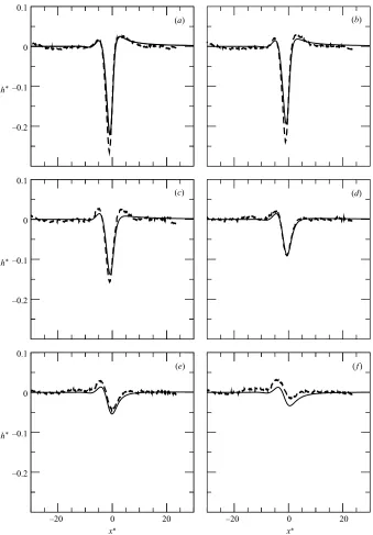
Figure 9. Comparison of predicted (full line) and experimental (dashed line) streamwise free-surface profile at different spanwise locations: (a) y∗= 0; (b) y∗=Lc/2; (c) y∗=Lc;

(d)y∗= 3Lc/2; (e)y∗= 2Lc; (f)y∗= 5Lc/2. The trench is square, and in this cross-section lies

in the region−0.776x∗60.77.

the present formulation, as demonstrated in figure 9, which compares corresponding streamwise profiles.

Figure 10.Flow of a thin water film over square topographies with w= 1.54, A= 1, and

|s0|= 0.25. In the three-dimensional views, the flow is from bottom-left to top-right: (a) trench; (b) peak. In the contour plots, flow is from left to right and the contours show free-surface height. Contour values are chosen to be equal in magnitude but opposite in sign: (c) trench; (d) peak. The crossed dashed lines indicate the centre of the topography and the arrow indicates the direction of flow.

the deeper depression over the trench itself, followed by a peak which Decr´e & Baret (2003) refer to as the ‘downstream surge’. This latter feature does not have an equivalent in the flow over one-dimensional topographies, and Decr´e & Baret (2003) admitted that its cause is not properly understood. The present authors believe that an explanation is provided by considering the flow rate into and out of the trench. Since the trench is finite in length and width, fluid will enter the trench both in the streamwise direction (over the upstream wall) and in the spanwise direction (over the sidewalls) due to lateral pressure gradients resulting from the spanwise curvature of the free surface. Since in a steady flow the fluid entering the trench must then leave it (over the downstream wall), the downstream surge simply arises to allow the fluid to exit the trench across a shorter width than that across which it entered. In the one-dimensional case there is no difference in the widths over which fluid enters and leaves the trench and therefore no cause for a downstream ridge.

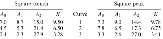
Square trench Square peak

A0 A1 A2 K Curve A0 A1 A2 K

7.0 8.7 15.0 9.50 1 7.3 9.0 14.4 9.78

4.5 5.3 21.4 6.50 2 7.8 6.5 17.3 6.75

2.4 2.3 27.9 3.28 3 3.3 2.6 27.0 3.41

Table 1. Curve fitting parameters for equations (4.1) and (4.2) corresponding to the curves labelled in figure 11. Note that the square-peak parameters are given for comparison only: the curves are not plotted in figure 11.

inversion of that over the trench. Decr´e & Baret (2003) did not consider peak-type topographies, but the plot in figure 10(b) is very similar to figure 3 in Hayes

et al. (2000) which gives the free surface produced in response to a Dirac delta peak

topography. Note that the downstream surge is now replaced by a depression (though this is not visible from the viewpoint in figure 10b). The above flow-rate argument can explain this feature too: fluid which passes over the top of the topography ascends the peak in the streamwise direction over the upstream wall, but is shed off the topography symmetrically by spanwise components over the sidewalls, leading to a reduced flow rate per unit width over the middle of the downstream wall and the consequent reduction in film thickness there.

Figures 10(c) and 10(d) show contour plots of free-surface height for the two topographies. The contour values are chosen to be equal in magnitude but opposite in sign, and show that the patterns produced are indeed very similar, but the surfaces are not quite mutual inverses. Again, the figures compare well with Decr´e & Baret’s figure 7 and figure 8 in Hayeset al. (2000) respectively.

The flows can be explored in more quantitative detail by examining the positions of spanwise local extrema in film thickness calculated by finding where ∂h∗/∂y∗= 0. Figure 11(a) shows the extrema for the trench and peak flows on the same plot, from which it is easy to see that the patterns produced are extremely close in shape but that there is a slight downstream shift between the two. This feature will be considered again later.

Guided by the form of Hayes et al.’s (2000) linear lubrication theory, Decr´e & Baret (2003) noted the self-similar behaviour of the film thickness with respect to y/x1/4 _{far downstream of the topography. This suggests that the downstream spread} of the extrema could be fitted by a power-law of the form

y∗=K(x∗)0.25

. (4.1)

However, while this expression does indeed describe the behaviour far enough downstream of the topography, it is of course not valid close to the origin (i.e. the topography) and cannot describe the shape of the bow wave upstream of the topography. An alternative fitting function takes the form

y=_±A1cosh−1

x₋A2 A0

+yt, (4.2)

20 40 60 80 100

y

d

1 2

3

0 20 40 60 80 100

0 20 40 60 80 100

0 20 40 60 80 100

x 20

40 60 80 100

y

1

2

3 20

40 60 80 100

y

(a)

(c) (b)

θ H0 Lc U0

(deg.) (µm) (mm) (mm s−1) wt s0 N

60 83.3 0.612 29.5 1.96 0.30 0.04

30 100.0 0.781 24.5 1.54 0.25 0.12

10 142.3 1.249 17.2 0.96 0.18 0.36

5 179.0 1.697 13.7 0.71 0.14 0.66

1 306.0 3.468 8.0 0.35 0.08 2.78

Table 2. Influence of inclination angle on various other parameters. The fluid properties and the flow rate per unit width are fixed at the following values for all angles:ρ= 1000 kg m−3_, µ= 0.001 Pa s,σ= 0.07 N m−1 _{andQ0= 1.635×10}−6_m2_s−1_.

and 3 correspond to spanwise local minima and curve 2 to the spanwise maxima of the upstream capillary ridge (cf. figure 10a). The data points to the left of curve 1 in figure 11(a, b) correspond to very slight ridges and depressions which cannot be resolved in figure 10(a) and are not considered further.

The two fitting expressions (4.1) and (4.2) are compared in figure 11(c). From approximately 10 capillary lengths downstream of the topography, the two sets of curves are practically indistinguishable. However, the clear distinction between the plots is that the inverse function (4.2) describes the positions of the spanwise extrema upstream of the topography and thus over the entire flow domain.

The function (4.2) provides useful insight into the behaviour of the capillary waves since they are predicted to meet the centreline y=yt at x=A0+A2 or, in physical coordinates, X0= (A0+A2)Lc. As the topography is centred at (Xt, Yt) = (xt, yt)Lc, it follows that the distance, d say – see figure 11(b) – between the point where the capillary wave intersects the centreline and the topography will be proportional to the capillary length and is given by d=Lc|xt−(A0+A2)|. This means that waves upstream of the topography are shifted further upstream whenLcincreases while those downstream of it are shifted further downstream. The former prediction is consistent with Mazouchi & Homsy’s (2001) finding, for one-dimensional topographies, that as capillary number decreases (i.e. Lc increases via equation (2.17)) the capillary ridge moves further upstream. Note that expression (4.2) applies equally well to the free-surface extrema in the flow over a square peak. Though not shown graphically, the fitting parameters for the peak are also given in table 1 for completeness.

While providing a very good description of wave spread, it should be noted that the function (4.2) does, however, have the disadvantage of requiring three parameters rather than one to provide a fit, and of course it does not predict the streamwise decay in amplitude available from the self-similar asymptotics.

Kalliadasiset al. (2000) demonstrated that in the flow over a one-dimensional step-up and step-down, increasing the normal component of gravity could reduce or even suppress entirely the capillary trough/ridge, making the free surface conform much more closely to the topography. In the present formulation, the parameter controlling the relative strength of this gravity component isN=Ca1/3_cot

–0.3

–10 0

10 20 –0.2

–0.1

0 ₍

a) (b)

(c) (d)

10

0

h*

h*

– y

– x

– y

– x

–0.3

–10 0

10 20 –0.2

–0.1 0

10

0

–0.3

–10 0

10 20 –0.2

–0.1 0

10

0 –0.3

–10 0

10 20 –0.2

–0.1 0

10

0

Figure 12.Close-up three-dimensional cut-away views illustrating the effect of inclination angle on the free surface generated in flow over the square trench of figure 10. (a) θ= 60◦ (N= 0.04), (b)θ= 10◦ _{(N= 0.36), (c)θ= 5}◦_{(N= 0.66), (d)θ= 1}◦ _{(N= 2.78). Note that since} Lc depends on θ, the in-plane coordinates are instead scaled by the (constant) topography width (see text) whileh∗ gives the deviation of the free surface from uniformity as a fraction of the topography depth. The topography is centred at (0,0), and the direction of flow is given by the arrow in each plot. The surface is symmetrical about ¯y= 0. See table 2 for the effect ofθ on other parameters.

and the effect of varying N in this way is shown in figures 12 and 13. Note that since Lc changes with θ, the in-plane coordinates are rescaled in terms of the fixed topography width. With reference to figure 1, the new coordinates (with origin at the topography) are given by (¯x,y¯) = (X₋XT, Y−YT)/WT.

Consistent with Kalliadasis et al. (2000), increasing N (i.e. decreasing θ) reduces and eventually eliminates the curved upstream capillary ridge. Other surface features are also dramatically reduced: the depression over the trench is much shallower, yet extends further upstream from the trench, and the downstream surge is much reduced in height, though it is still present. When interpreting these results, however, one should bear in mind thatH0 increases asθ decreases (table 2), and the free surface is expected to become less sensitive to the topography for thicker films.

–10 –5 0 5 10 15 –0.3

–0.2 –0.1 0

h*

60°

30°

10°

5°

1°

0 20 40

–20 0 20

– y

– x

– x 1

3

2 1

1

2 2

3 3

Figure 13. The effect of θ on the amplitude and spread of the disturbance created by the square trench of figure 10. As in figure 12, the in-plane coordinates are scaled with the topography width rather than Lc since the latter is dependent on θ. The main plot shows streamwise profiles taken along ¯y= 0, with the topography indicated by the thick solid line at the bottom – note, however, that the height of the topography is not shown at its true value: it in fact lies ath∗=₋1/s0. The inset graph shows the positions of local extrema in film thickness, i.e. points at which ∂h∗/∂y¯= 0, and the small square at (0,0) indicates the position and extent of the topography. The same legend applies to both the main and inset graphs. The numbers 1, 2, 3 label corresponding extrema for each angle – see also figure 11(b, c).

Returning to theθ= 30◦_{,N= 0.12 flow, figure 14 demonstrates the effect of}

increas-ing the aspect ratio,A, of the trench by extending its spanwise length. The viewpoint chosen for these visualizations is on the opposite side of the topography to that in figures 10 and 12, giving a reverse view of the free-surface disturbance. When A is increased to 5 (figure 14b), the depth of the depression over the trench is greatly increased and the height of the curved capillary ridge upstream of the topography is also increased. The central downstream surge is still clearly present, though it decays in amplitude more slowly than that following the square trench. Increasing Ato 8.33 widens the upstream ridge, and introduces a bifurcation in the downstream surge such that two smaller surges lie either side of the centreline of the topography, see figure 14(c). As A increases further, the free surface appears to become flat in the central region just downstream of the trench; coupled with the flattening of the top of the upstream ridge (figure 14d), this shows that the flow near to the centrelinex∗= 0 approximates closely that over a one-dimensional trench. The above observations are clarified by overlaying the centreline profiles as in figure 15.

–50 –25 –0.4 –0.2 0

(a)

h* –25 0 0 25 25 50 50 –50 –25 –0.4 –0.2 0

(b)

–25 0 0 25 25 50 50 –50 –25 –0.4 –0.2 0

(c)

h*

y* x*

–25 0 0 25 25 50 50 –50 –25 –0.4 –0.2 0

(d)

y* x*

–25 0 0 25 25 50 50

Figure 14.Three-dimensional rear-view of the free surface generated by flow (from top-right to bottom-left) over trenches, showing the effect of trench aspect ratio on the downstream surge. (a)A= 1; (b)A= 5; (c)A= 8.33; (d)A= 15.

–50 –30 –10 10 30 50

y* –0.5 –0.3 –0.1 0.1 spanwise

A = 15

A = 8.33

A = 5 A = 1

–30 –10 10 30 50

x* –0.7 –0.5 –0.3 –0.1 0.1 0.3 h*

(a) (b)

Figure 15.Effect of topography aspect ratio on (a) streamwise free-surface profiles y∗= 0, and (b) spanwise free-surface profiles alongx= 0. For comparison, the profiles for flow over the corresponding one-dimensional spanwise trench are also given.

–20 –10 0 10 20 30 x*

–0.5 –0.4 –0.3 –0.2 –0.1 0 0.1 0.2

h*

Linear superposition (numerical) LT = 1.52 Lc, A = 5 (numerical) Linear superposition (Decré & Baret 2003) Experiment (Decré & Baret 2003)

Figure 16. Streamwise free-surface profiles for a spanwise trench of aspect ratio 5: comparison between the full numerical solution and a linear superposition of five suitably shifted solutions for flow over a square trench. Also shown are the direct experimental measurements and corresponding superposition of square-trench measurements from Decr´e & Baret (2003).

The near-linearity of the results in figure 16 and in Decr´e & Baret (2003) supports the observation by those authors that linear superposition of the responses to elemen-tary topographies can reliably construct the response to more complex topographies – at least for flow conditions similar to those considered here. The accuracy of the linear superposition is perhaps most rigorously tested by adding together the solutions corresponding to a pair of equal but opposite topographies, i.e. a trench and a peak, since if the response of the free surface to topographic features is linear, the resulting surface should be planar. From the analysis of Stillwagon & Larson (1990), such a linear response is to be expected in the limits of very small Ca, when the free surface is almost planar, or largerCaif the height (depth) of the topography is much smaller than the film thickness (i.e. _|s0| ≪1).

–10 0 10 20 x*

–10 0 10 20

x* –0.3

–0.2 –0.1 0 0.1 0.2 0.3

25 ₂₅

50 –0.01

0.01 (a)

(b) (c)

50

0

0 –25

–25 –50

h*

h*

y* x*

peak trench

linear superposition

–0.3 –0.2 –0.1 0 0.1 0.2 0.3

Figure 17.Superposition of the free surfaces generated by flows over equal but opposite square topographies with w= 1.54. (a) Three-dimensional view of the constructed surface when |s0|= 0.25; (b) streamwise free-surface profiles along y∗= 0 compared to those of the individual flows with|s0|= 0.25; (c) as (b) but with|s0|= 0.1.

to be more linear, the variation in the constructed profile is indeed reduced – to below 2%.

Finally, an example is given in figure 18 of an attempt to reduce the free-surface disturbance caused by a square peak topography by modifying the topography surrounding the peak. In this case, a simple shallow trench is created around the peak; the topography sizes are given in the figure. The streamwise profile along the centreline (figure 18b) shows that although the composite topography produces a deeper depression in the free surface, the overall disturbance is smaller (the r.m.s. deviation over the whole domain is 0.62% for the peak alone and 0.26% for the peak with a trench). In addition, the film thickness relaxes more quickly to equilibrium downstream of the trench. The contour plots (figure 18c, d) also show that the region of maximum disturbance is smaller for the composite topography, despite its greater extent.

–5 0 5 10 15 20 25 30 –10

–5 0 5 10

–5 0 5 10 15 20 25 30

–10 –5 0 5 10

–30 –10 10 30 50 70

x* –0.2

–0.1 0 0.1 0.2 0.3 0.4

h*

y*

x*

4.62

4.62 1.54

1.54

s0 = 0.25

s0 = –0.05 (a)

(c)

(b) _(d)

Figure 18. Reducing the free-surface disturbance caused by a square peak by surrounding the peak by a shallow trench: (a) geometry of the composite topography; (b) streamwise profile alongy∗= 0 for the square peak alone (solid line) and the composite topography (dashed line); (c) contours of free-surface height generated by the peak alone; (d) corresponding contours for the composite topography.

5. Conclusions

Thin film flow over various one- and two-dimensional topographies has been studied by means of finite element solutions of the Navier–Stokes equations and multigrid finite difference predictions based on lubrication theory. In the one-dimensional case, Stokes solutions for the flow over a wide trench were shown to be in excellent agreement with those of Mazouchi & Homsy (2001), and Navier–Stokes solutions with Re= 10 revealed that the effect of increasingRe is to increase the amplitude of the free-surface disturbances while slightly reducing their wavelength.

The discussion of three-dimensional flow focused mainly on that over a square trench, calculated using lubrication theory. The predicted free-surface shapes agree well with the experiments of Decr´e & Baret (2003), and particular thought was given to the cause of the ‘downstream surge’ which is not present in the flow over one-dimensional topographies. A simple explanation for the elevated surface behind the trench is that fluid flows into the trench across a greater width (i.e. over the upstream and side walls) than that across which it must exit. The depression in the free surface behind a square peak topography can be similarly explained. The normal component of gravity was shown to suppress the upstream free-surface disturbance, as expected from the one-dimensional analysis of Kalliadasiset al. (2000), but it does not completely inhibit the downstream surge. This is consistent with the above explanation for the appearance of the surge. Three-dimensional rear-view visualizations of the free surface showed how the downstream surge separates into two as the aspect ratio of the trench is increased and how the flow over the centre of the trench approaches the one-dimensional case.

The positions of the spanwise local extrema in film thickness produced by flow past a square trench and an equal but opposite square peak were plotted as a function of the in-plane coordinates, and an inverse hyperbolic cosine function was demonstrated to fit these loci extremely well even upstream of the topography. This gives a complete description of the spread of the bow wave, but does not capture the rate of decay in amplitude. The equal square peak and trench were used to test the linearity of the free-surface response to topography by superimposing the individual responses to see if the surface produced was planar. While not being perfectly planar, there was only a slight deviation of the order of 7% of the individual disturbances when the topography depth was a quarter of the film thickness. Reducing the relative depth of the topography to 0.1 resulted in an even smaller deviation of the order of 2%.

An example was also given of a modification to a square-peak topography which substantially reduces the free-surface disturbance caused by it. Such modifications of essential topographic features may help to minimize troublesome free-surface features at later stages in manufacturing processes.

The authors are grateful to Philips Electronics, Eindhoven, for sponsoring this work and to Michel Decr´e and Jean-Christophe Baret in particular for their keen interest in the subject matter, and for providing their experimental data in electronic form for comparison purposes.

REFERENCES

Aksel, N.2000 Influence of the capillarity on a creeping flow down an inclined plane with an edge. Arch. Appl. Mech.70, 81–90.

Bertozzi, A. & Brenner, M. P.1997 Linear stability and transient growth in driven contact lines. Phys. Fluids 9_{, 530–539.}

Brandt, A.1977 Multi-level adaptive solutions to boundary-value problems.Maths Comput.31-138_, 333–390.

Christodoulou, K. N., Kistler, S. F. & Schunk, P. R. 1997 Advances in computational methods for free surface flows. InLiquid Film Coating(ed. S. F. Kistler & P. M. Schweizer), pp. 297–366. Chapman and Hall.

Christodoulou, K. N. & Scriven, L. E.1989 The fluid mechanics of slide coating.J. Fluid Mech. 208_{, 321–354.}

Decr´e, M. M. J., Fernandez-Parent, C. & Lammers, J. H. 1998 Flow of a gravity driven thin liquid film over one-dimensional topographies.Philips Research, Unclassified Report NL-UR 823/98.

Decr´e, M. M. J., Fernandez-Parent, C. & Lammers, J. H.1999 Flow of a gravity driven thin liquid film over one-dimensional topographies: a tripartite approach. Proc. 3rd European Coating Symposium (ed. F. Durst & H. Raszillier), pp. 151–156. Springer.

Fawehinmi, O. B., Gaskell, P. H. & Thompson, H. M.2002 Finite element analysis of flow in a cavity with internal blockages.Proc. Inst. Mech. Engrs C216_{, 517–530.}

Gaskell, P. H., Jimack, P. K., Sellier, M. & Thompson, H. M. 2004 Efficient and accurate time-adaptive multigrid simulations of droplet spreading. Intl J. Numer. Meth. Fluids (In press).

Gaskell, P. H., Savage, M. D., Summers, J. L. & Thompson, H. M. 1995 Modelling and analysis of meniscus roll coating.J. Fluid Mech.298_{, 113–137.}

Gaskell, P. H., Savage, M. D., Summers, J. L. & Thompson, H. M. 1998 Stokes flow in closed, rectangular domains.Appl. Math. Modelling 22_{, 727–743.}

Gaskell, P. H., Savage, M. D. & Wilson, M. 1997 Stokes flow in a half filled annulus between rotating coaxial cylinders.J. Fluid Mech.337_{, 263–282.}

Gramlich, C. M., Kalliadasis, S., Homsy, G. M. & Messer, C. 2002 Optimal levelling of flow over one-dimensional topography by Marangoni stresses.Phys. Fluids 14_{, 1841–1850.} Hayes, M., O’Brien, S. B. G. & Lammers, J. H. 2000 Green’s function of steady flow over a

two-dimensional topography.Phys. Fluids 12, 2845–2858.

Heil, M.2000 Finite Reynolds number effects in the propagation of an air finger into a liquid-filled flexible-walled channel.J. Fluid Mech.424, 21–44.

Higdon, J. J. L.1985 Stokes flow in arbitrary two-dimensional domains: shear flow over ridges and cavities.J. Fluid Mech.159_{, 195–226.}

Hood, P.1976 Frontal solution program for unsymmetric matrices.Intl J. Numer. Meth. Engng 10_, 379–399.

Kalliadasis, S., Bielarz, C. & Homsy, G. M. 2000 Steady free-surface thin film flow over two-dimensional topography.Phys. Fluids 12_{, 1889–1898.}

Kalliadasis, S. & Homsy, G. M. 2001 Stability of free surface thin-film flows over topography. J. Fluid Mech.448_{, 387–410.}

Kelmanson, M. A. & Lonsdale, B.1996 Eddy genesis in the double-lid-driven cavity.Q. J. Mech. Appl. Maths 49_{, 635–655.}

Kistler, S. F. & Scriven, L. E.1983 Coating flows. InComputational Analysis of Polymer Processing (ed. J. R. A. Pearson & S. M. Richardson), Chap. 8, pp. 243–299. Applied Science Publishers. Kistler, S. F. & Schweizer, P. M.1997Liquid Film Coating. Chapman and Hall.

Luc´ea, M., Decr´e, M. M. J. & Lammers, J. H.1999 Flow of a gravity driven thin liquid film over topographies.Philips Research, Unclassified Report NL-UR 833/99.

Mazouchi, A. & Homsy, G. M. 2001 Free surface Stokes flow over topography.Phys. Fluids 13_, 2751–2761.

Mess´e, S. & Decr´e, M. M. J.1997 Experimental study of a gravity driven water film flowing down inclined plates with different patterns.Philips Research, Unclassified Report NL-UR 030/97. Peurrung, L. M. & Graves, B. G.1991 Film thickness profiles over topography in spin coating.

J. Electrochem. Soc.138_{, 2115–2124.}

Peurrung, L. M. & Graves, B. G.1993 Spin coating over topography.IEEE Trans. Semi. Man.6_, 72–76.

Pozrikidis, C. & Thoroddsen, S. T.1991 The deformation of a liquid film flowing down an inclined plane wall over a small particle arrested on the wall.Phys. Fluids A3_{, 2546–2558.}

Pritchard, W. G., Scott, L. R. & Tavener, S. J. 1992 Numerical and asymptotic methods for certain viscous free-surface flows.Phil. Trans. R. Soc. Lond.A340_{, 1–45.}

Roy, R. V. & Schwartz, L. W. 1997 Coating flow over a curved substrate. Proc. 2nd European Coating Symposium (ed. P. G. Bourgin), pp. 18–27. Universit´e Louis Pasteur, Strasbourg. Shankar, P. N. & Deshpande, M. D.2000 Fluid mechanics in the driven cavity.Annu. Rev. Fluid

Mech.32, 93–136.

Stillwagon, L. E. & Larson, R. G.1988 Fundamentals of topographic substrate levelling.J. Appl. Phys.63_{, 5251–5228.}

Stillwagon, L. E. & Larson, R. G.1990 Leveling of thin films over uneven substrates during spin coating.Phys. Fluids A2_{, 1937–1944.}

Summers, J. L., Thompson, H. M. & Gaskell, P. H.2004 Flow structure and transfer jets in a contra-rotating rigid-roll coating system.Theor. Comput. Fluid Dyn.17, 189–212.