arXiv:hep-ph/0407238v1 21 Jul 2004
One loop MS gluon pole mass from the LCO formalism
R.E. Browne & J.A. Gracey, Theoretical Physics Division, Department of Mathematical Sciences,
University of Liverpool, P.O. Box 147,
Liverpool, L69 3BX, United Kingdom.
Abstract. We compute the one loop corrections to the pole mass of the gluon in the MS scheme in the Landau gauge in both the Curci-Ferrari model and the local composite operator formalism withNf flavours of massless quarks. For the latter we determine an estimate for the gluon mass
using the effective potential of a local dimension two composite operator and find, for example, mgluon = 2·10ΛMS in Yang-Mills theory.
The issue of whether the gluon obtains a dynamically generated mass has been a popular topic of investigation in recent years. Following the work of [1, 2, 3, 4] who observed that the perturbative vacuum of QCD is unstable, one of the main activities has been on the numerical evaluation of the vacuum expectation value of the square of the gauge potential,h1
2A
2
µi. Various
methods have been used to achieve this ranging from combinations of lattice computations with the operator product expansion and instanton considerations, [5, 6, 7, 8, 9, 10, 11], to a more theoretical approach of the local composite operator formalism of, for instance, [12, 13, 14, 15]. Moreover, there is evidence from phenomenology that the existence of a gluon mass in the range of 500-800 MeV may provide a more accurate explanation of various experimental data. Indeed, a valuable summary table of current gluon mass estimates has been given in the article by Field, [16]. Whilst the operator 1
2A
2
µ suffers from the immediate objection of not being a
gauge invariant entity, it has been shown how to relate it to a dimension two gauge invariant physical operator, which is the minimization ofA2µover all gauge configurations [12, 17, 18].This operator, albeit non-local, reduces to a local operator in the Landau gauge and it is solely in this gauge that, for example the lattice results of [5, 6, 10, 11] have been determined. Indeed the local composite operator (LCO) formalism of [12, 13] was originally developed in the Landau gauge but recently an estimate ofh1
2A
2
µihas been determined in arbitrary linear covariant gauge,
[17].
Whilst there is much activity in trying to ascertain the existence of a dynamical gluon mass, there appears to be less effort into standardizing mass estimates. For instance, in the quark sector of QCD the estimates of the various quark masses by methods such as sum rules, lattice regularization and the operator product expansion are all expressed as the MS running mass at the scale of 2GeV. Although clearly measurements are not always made at this scale. To connect the mass estimates one requires an as accurate as possible evaluation in perturbation theory of the quark mass anomalous dimension in the MS scheme. This is currently available at four loops, [19, 20, 21, 22, 23]. Moreover, the relation between the quark pole masses and the running mass is known at three loops, [24]. For the same problem for a gluon mass the analogous quantities are not available to as high an order. For instance, the running of the naive gluon mass operator, 1
2A
2
µ −αcc¯ , in the non-linear Curci-Ferrari gauge, [25], is known at three
loops, [26]. In the Landau gauge, it transpires that it is not an independent renormalization being the sum of the gluon and ghost anomalous dimensions, which is a result that derives from a Slavnov-Taylor identity, [27]. This has recently been exploited to obtain the four loop running in the Landau gauge for the SU(3) colour group, [28]. However, the relation between the pole mass of the gluon and the running gluon mass is not yet available for QCD at one loop. Therefore, it is the aim of this article to provide such a relation for QCD which will build on the Yang-Mills expression recently given in [29] for the Curci-Ferrari gauge. Moreover, since the LCO formalism has provided estimates for a dynamically generated gluon mass which are comparable with other methods we will also determine the relation for that approach as well. This will provide a clean estimate for a gluon mass, since in [12] the effective potential for the operator 1
2A
2
µ was developed at two loops in the Landau gauge. However, there the estimate for
a dynamical gluon mass was based on determining the value of an effective gluon mass which was by definition a classical mass. It seems to us that a more appropriate quantity to estimate through the effective potential approach would be a one loop quantity derived from the gluon two-point function such as the pole mass. This is the second aim of the article.
We begin by defining our notation. We recall that the QCD Lagrangian in a linear covariant gauge is
LQCD = − 1 4G
a
µνGa µν −
1 2α(∂
µAa
µ)2 − ¯ca∂µDµca + iψ¯iID/ψiI (1)
field. The indices take the following ranges 1≤a≤NA, 1≤I ≤NF and 1≤i≤Nf whereNF
and NA are the dimensions of the fundamental and adjoint representations respectively, Nf is
the number of quark flavours andfabc are the colour group structure constants. The covariant derivatives which determine Ga
µν are
Dµca = ∂µca − gfabcAbµcc , DµψiI = ∂µψiI + igTaAaµψiI . (2)
In [12], the LCO formalism was derived which involves an additional scalar field σ which is related to the dimension two composite operator 1
2A
2
µ. The relevant Lagrangian is
LLCO = LQCD − σ
2
2g2ζ(g) +
1 2gζ(g)σA
a
µAa µ −
1 8ζ(g)
AaµAa µ2 (3)
where there is an extra contribution to the quartic gluon interaction and LLCO contains the usual covariant gauge fixing terms though we will only consider the Landau gauge case,α = 0. The quantity ζ(g) is a function of the coupling constant which has been computed to O(g2) in the Landau gauge in [12, 13, 14] and is such that it ensures the generating functional underlying the formalism satisfies a homogeneous renormalization group equation, [12]. For this article we note that the relevant terms are
1 g2ζ(g) =
(13C
A−8TFNf)
9NA
+ 2685464CA3TFNf −1391845CA4 −213408CA2CFTFNf −1901760CA2TF2Nf2
+ 221184CACFTF2Nf2+ 584192CANf3TF3 −55296CFTF3Nf3
− 65536TF4Nf4 g
2
5184π2N
A(35CA−16TFNf)(19CA−8TFNf)
#
. (4)
In [12, 13, 14] theσ field develops a non-zero vacuum expectation value when one computes the one loop effective potential of σ which is
V(σ) = 9NA 2 λ1σ
′2
+
3
64ln
gσ′
µ2
+CA
− 3518 CFλ1λ2+
351
16 CFλ1λ3− 249 128λ2+
27 64λ3
+ CA2
− 8116λ1λ2+
81 32λ1λ3
+
− 12813 − 20732 CFλ2+
117 32 CFλ3
g2N
Aσ′2
π2 + O(g
4) (5)
where we have set
λ1 = [13CA−8TFNf]−1 , λ2 = [35CA−16TFNf]−1 , λ3 = [19CA−8TFNf]−1 , (6)
σ = 9NA (13CA−8TFNf)
σ′ (7)
and µ is the usual MS renormalization scale, which is introduced to retain a dimensionless coupling constant in dimensional regularization.
Now we consider the relation between the pole mass and the running gluon mass in the Curci-Ferrari model, [25], which includes the BRST invariant mass operator
Lmass = 1 2m
2Aa
wherem is the bare mass. With this term the gluon and ghost propagators in the Landau gauge are
− δ ab
(k2−m2)
ηµν −
kµkν
k2
, δ
ab
k2 (9)
respectively. With these it is a straightforward exercise to compute the one loop correction to the gluon two-point function. In this respect the one loop snail diagram derived from the quartic gluon interaction cannot be neglected in the massive case. The result of our computation for the pole mass in the Curci-Ferrari model is
m2CF =
" 1 + 313 576 − 35 192ln
m2(µ)
µ2
!
− 11π √ 3 128 ! CA + 1 12ln
m2(µ)
µ2
!
−365
!
TFNf
!
g2
π2 + O(g
4)
#
m2(µ) (10)
where mo = m(µ)Zm is the bare mass, m(µ) is the running mass and µis the renormalization
mass scale. We have renormalized with the usual one loop MS renormalization constants. As a check on the expression, we note that it reduces to the same relation given in [29] whenNf = 0.
Moreover, we have verified the expression of [29] for arbitraryα prior to specifying the Landau gauge which provided a non-trivial check on the symbolic manipulation programmes we used for this article.
We have repeated the above computation for the LCO Lagrangian where the bare mass is now defined to beσ/[gζ(g)], [12, 13, 14], which at leading order is
m2o = (13CA−8TFNf) 9NA
gσ . (11)
With the additional interactions the expression for the LCO pole mass is of a similar form
m2LCO =
" 1 + 287 576 − 3 64ln
m2(µ) µ2
!
− 11π √
3 128
!
CA
− 19TFNf
g2
π2 + O(g
4)
#
m2(µ) (12)
for massless quarks in the Landau gauge. Equipped with this result we can now extend the method of [12, 13, 14] for estimating a gluon mass. In [12, 14] the minimum of the effective potential (5) was determined by solving dVdσ(σ) = 0. Since the factors multiplying the classi-cal effective mass are coupling constant dependent, this is equivalent to extremizing Veff(m2o). However, it seems to us that an alternative approach is to compute instead the extremum of Veff(m2
LCO) where one inverts (12) to obtainm(µ) as a function ofm2LCO and then substitutes this into (5). Thus we find
Veffm2LCO =
9
2λ1+
−12829 −20732 CFλ2+
117 32 CFλ3 + CA
−3518 CFλ1λ2+
351
16 CFλ1λ3− 183
64 λ1
− 249128λ2+27
64λ3+ 99 128π
√
3λ1
+ CA2
−8116λ1λ2+
81 32λ1λ3
+ 3 64ln m2 LCO µ2 ! + 27
64CAλ1ln
m2LCO µ2
!!
g2 π2
#
(13CA−8TFNf)2
81NA
Repeating the process to find a minimum necessitates solving
0 =
9
2λ1+
−1364 −20732 CFλ2+
117 32 CFλ3 + CA
−3518 CFλ1λ2+
351
16 CFλ1λ3− 339 128λ1
− 249128λ2+
27 64λ3+
99 128π
√
3λ1
+ CA2
−8116λ1λ2+
81 32λ1λ3
+ 3 64ln
m2
LCO µ2
!
+ 27
64CAλ1ln
m2LCO µ2
!!
g2 π2
#
(13CA−8TFNf)2
81NA
g2ζ2(g)m4LCO (14)
which corresponds to the condition
dV m2
LCO
dm2
LCO
= 0. (15)
We have not in fact substituted for the explicit expression for ζ(g) since this function factorizes off the expression for the location of the minimum. If we were to include that part of the series which was already known it would introduce an unnecessary truncation error into our final estimates for the pole mass. At this point to solve for the mass a scale needs to be chosen for µ. In [12, 13, 14], the choice of scale was such that it removed the logarithm terms. For this potential we will take a more general approach and instead set m2
LCO = sµ2 wheres is an arbitrary parameter. This means we have determined an equation for the value of the coupling constant as a function of s. In other words
y = 36CA(16TFNf −35CA)
h
3465π√3 + 4620 ln(s)−25690CA2 −864CFTFNf
+ 19240−1584π√3−3792 ln(s)CATFNf
+ (768 ln(s)−3328)TF2Nf2i−1 (16)
where y =CAg2/(16π2). Through the definition of the running coupling constant we have the
one loop relation
g2(µ) 16π2 =
"
β0ln
"
µ2 Λ2
MS
##−1
(17)
where
β0 =
11 3 CA −
4
3TFNf . (18)
Hence, we can relate the coupling constant to the scaleµand ΛMS and deduce a value form2LCO. We find
mLCO = Λ(Nf)
MS exp
h
− 3465π√3−25690CA2 −864CFTFNf
+ 19240−1584π√3CATFNf − 3328TF2Nf2
24 (11CA−4TFNf) (35CA−16TFNf)
−1#
(19)
Nf mSU(2)/Λ
(Nf)
MS mSU(3)/Λ
(Nf)
MS
0 2.10 2.10
2 1.54 1.74
[image:6.612.206.391.79.140.2]3 1.24 1.55
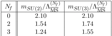
Table 1. One loop estimates of the gluon effective mass forSU(2) andSU(3).
We have given the explicit values of the pole mass estimates from (19) forSU(2) andSU(3) in Table 1. Compared with the classical effective gluon mass estimates of [12, 13, 14] the Yang-Mills estimates have increased by about 5% forSU(3). However, forNf 6= 0 there is a significant
decrease. Although this is disappointing it is important to recognise that since they have been derived in a scale independent and therefore renormalization group invariant manner, they may be closer to the true result, though the inclusion of quark mass may alter these estimates.
We conclude with several remarks. First, we have constructed a one loop renormalization group invariant pole mass for the gluon using the LCO effective potential of [12, 13, 14]. However, it would be interesting to see whether this feature persists at the next order. This only requires an extension of the present one loop result since the two loop LCO effective potential is available. Although we have ignored quark mass effects it seems that if one could include quark condensates in the LCO formalism in addition to that for 1
2A
a µAa
µ then it might be possible to ascertain
the extent to which condensates could be responsible for the quark and gluon masses. If the renormalization scale invariance persists even at one loop for this scenario then one would not have to worry about solving a multi-scale type renormalization group equation. Our final comment concerns the situation where a gluon mass is dynamically generated through, say, the LCO formalism. If this is the case then one would have to include additional contributions due to a gluon mass to the existing quark pole mass multi-loop estimates.
Acknowledgement. This work was supported in part by PPARC through a research
stu-dentship, (REB). We also thank Prof D.R.T. Jones and Dr C. McNeile for discussions.
References.
[1] G.K. Savvidy, Phys. Lett. B71 (1977), 133.
[2] V.P. Gusynin & V.A. Miransky, Phys. Lett.B76 (1978), 585.
[3] R. Fukuda & T. Kugo, Prog. Theor. Phys.60(1978), 565.
[4] R. Fukuda, Phys. Lett.B73 (1978), 33; Phys. Lett. B74(1978), 433.
[5] P. Boucaud, A. Le Yaouanc, J.P. Leroy, J. Micheli, O. P`ene & J. Rodriguez-Quintero, Phys. Rev. D63(2001), 114003.
[6] P. Boucaud, J.P. Leroy, A. Le Yaounac, J. Micheli, O. P`ene, F. De Soto, A. Donini, H. Moutarde & J. Rodriguez-Quintero, Phys. Rev.D66 (2002), 034504.
[7] K.I. Kondo, T. Murakami, T. Shinohara & T. Imai, Phys. Rev. D65 (2002), 085034.
[9] M.J. Lavelle & M. Oleszczuk, Mod. Phys. Lett.A7 (1992), 3617.
[10] P. Boucaud, G. Burgio, F. Di Renzo, J.P. Leroy, J. Micheli, C. Parrinello, O. P`ene, C. Pittori, J. Rodriguez-Quintero, C. Roiesnel & K. Sharkey, JHEP0004 (2000), 006.
[11] D. Becirevic, P. Boucaud, F. De Soto, A. Le Yaouanc, J.P. Leroy, J. Micheli, O. P`ene, J. Rodriguez-Quintero & C. Roiesnel, Nucl. Phys. Proc. Suppl.106 (2002), 867.
[12] H. Verschelde, K. Knecht, K. van Acoleyen & M. Vanderkelen, Phys. Lett. B516 (2001), 307; erratum.
[13] K. Knecht, ‘Algoritmische multiloop berekeningen in massieve kwantumveldentheorie’ Uni-versity of Gent PhD thesis.
[14] R.E. Browne & J.A. Gracey, JHEP 11(2003), 029.
[15] D. Dudal, H. Verschelde, J.A. Gracey, V.E.R. Lemes, M.S. Sarandy, R.F. Sobreiro & S.P. Sorella, JHEP01 (2004), 044.
[16] J.H. Field, Phys. Rev. D66 (2002), 013013.
[17] K.I. Kondo, Phys. Lett.B572 (2003), 210.
[18] M. Esole & F. Friere, hep-th/0401055.
[19] D.V. Nanopoulos & D.A. Ross, Nucl. Phys.B157 (1979), 273.
[20] R. Tarrach, Nucl. Phys.B183(1981), 384; O. Nachtmann & W. Wetzel, Nucl. Phys.B187
(1981), 333.
[21] O. Tarasov, JINR preprint P2-82-900.
[22] J.A.M. Vermaseren, S.A. Larin & T. van Ritbergen, Phys. Lett.B405 (1997), 327.
[23] K.G. Chetyrkin, Phys. Lett.B404 (1997), 161.
[24] N. Gray, D.J. Broadhurst, W. Grafe & K. Schilcher, Z. Phys. C48(1990), 673.
[25] G. Curci & R. Ferrari, Nuovo Cim. A32(1976), 151.
[26] J.A. Gracey, Phys. Lett.B552 (2003), 101.
[27] D. Dudal, H. Verschelde & S.P. Sorella, Phys. Lett.B555 (2003), 126.
[28] K.G. Chetyrkin, hep-ph/0405193.