A novel artificial immune algorithm for spatial clustering with obstacle constraint and its applications

Research Article

A Novel Artificial Immune Algorithm for Spatial Clustering with

Obstacle Constraint and Its Applications

Liping Sun,

Yonglong Luo,

Xintao Ding,

and Ji Zhang

2_{Engineering Technology Research Center of Network and Information Security, Anhui Normal University, China} 3_{Faculty of Health, Engineering and Sciences, University of Southern Queensland, Australia}

Correspondence should be addressed to Yonglong Luo; [email protected]

Received 18 July 2014; Accepted 23 August 2014; Published 4 November 2014

Academic Editor: Jianjun Yang

Copyright © 2014 Liping Sun et al. This is an open access article distributed under the Creative Commons Attribution License, which permits unrestricted use, distribution, and reproduction in any medium, provided the original work is properly cited.

An important component of a spatial clustering algorithm is the distance measure between sample points in object space. In this paper, the traditional Euclidean distance measure is replaced with innovative obstacle distance measure for spatial clustering under obstacle constraints. Firstly, we present a path searching algorithm to approximate the obstacle distance between two points for dealing with obstacles and facilitators. Taking obstacle distance as similarity metric, we subsequently propose the artificial immune clustering with obstacle entity (AICOE) algorithm for clustering spatial point data in the presence of obstacles and facilitators. Finally, the paper presents a comparative analysis of AICOE algorithm and the classical clustering algorithms. Our clustering model based on artificial immune system is also applied to the case of public facility location problem in order to establish the practical applicability of our approach. By using the clone selection principle and updating the cluster centers based on the elite antibodies, the AICOE algorithm is able to achieve the global optimum and better clustering effect.

1. Introduction

Spatial clustering analysis is an important research problem in data mining and knowledge discovery, the aim of which is to group spatial data points into clusters. Based on the simi-larity or spatial proximity of spatial entities, the spatial dataset is divided into a series of meaningful clusters [1]. Due to the spatial data cluster rule, clustering algorithms can be divi-ded into spatial clustering algorithm based on partition [2,3], spatial clustering algorithm based on hierarchy [4,5], spatial clustering algorithm based on density [6], and spatial cluster-ing algorithm based on grid [7].

The distance measure between sample points in object space is an important component of a spatial clustering algo-rithm. The above traditional clustering algorithms assume that two spatial entities are directly reachable and use a variety of straight-line distance metrics to measure the degree of similarity between spatial entities. However physical barriers often exist in the realistic region. If these obstacles and facil-itators are not considered during the clustering process, the clustering results are often not realistic. Taking the simulated

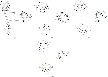
dataset in Figure1(a)as an example, where the points repre-sent the location of consumers, the clustering result shown in Figure1(b)can be obtained, when the rivers and hill as obstacles are not considered. If the obstacles are taken into account and bridges as facilitators are not considered, the clustering result in Figure1(c)can be gained. Considering both the obstacles and facilitators, Figure1(d)demonstrates the more efficient clustering patterns.

At present, only a few clustering algorithms consider obstacles and/or facilitators in the spatial clustering process. COE-CLARANS algorithm [8] is the first spatial clustering algorithm with obstacles constraints in a spatial database, which is an extension of classic partitional clustering algo-rithm. It has similar limitations to the CLARANS algorithm [9], which has sensitive density variation and poor efficiency. DBCluC [10] extends the concepts of DBSCAN algorithm [11], utilizing obstruction lines to fill the visible space of obstacles. However, it cannot discover clusters of different densities. DBRS+ is the extension of DBRS algorithm [12], considering the continuity in a neighborhood. Global parameters used by DBRS+ algorithm make it suffer from

River

Hill Bridge

(a)

C1

C2

C3

(b)

C1 _C

2

C3 _C

4

C5

C6

(c)

C1

C2

C3

C4

C5

(d)

Figure 1: Spatial clustering with obstacle and facilitator constraints: (a) spatial dataset with obstacles; (b) spatial clustering result ignoring obstacles; (c) spatial clustering result considering obstacles; (d) spatial clustering result considering both obstacles and facilitators.

the problem of uneven density. AUTOCLUST+ is a graph-based clustering algorithm, which is graph-based on AUTOCLUST clustering algorithm [13]. For the statistical indicators used by AUTOCLUST+ algorithm, it could not deal with planar obstacles. Liu et al. presented an adaptive spatial clustering algorithm [14] in the presence of obstacles and facilitators, which has the same defect as AUTOCLUST+ algorithm.

Recently, the artificial immune system (AIS) inspired by biological evolution provides a new idea for clustering anal-ysis. Due to the adaptability and self-organising behaviour of the artificial immune system, it has gradually become a research hotspot in the domain of smart computing [15–20]. Bereta and Burczy´nski performed the clustering analysis by means of an effective and stable immune𝐾-means algorithm for both unsupervised and supervised learning [21]. Gou et al. proposed the multielitist immune clonal quantum clustering algorithm by embedding a potential evolution formula into affinity function calculation of multielitist immune clonal optimization and updating the cluster center based on the distance matrix [22]. Liu et al. put forward a novel immune clustering algorithm based on clonal selection method and immunodominance theory [23].

In this paper, a path searching algorithm is firstly pro-posed for the approximate optimal path between two points among obstacles to achieve the corresponding obstacle dis-tance. It does not need preprocessing and can deal with both

linear and planar obstacles. Based on the path searching algo-rithm, a spatial clustering algorithm is proposed to the spatial data clustering in the presence of both obstacles and facili-tators. A case study is also carried out to apply our method to the problem of public facility optimization.

The remainder of this paper is organized as follows. Sec-tion2at first presents the path searching algorithm and then elaborates the details of AICOE algorithm, including analysis of population partition, the design of affinity function, and immune operators. Section3shows the experimental results. Section4presents the conclusions and main findings.

2. Theoretical Framework

2.1. Obstacles Representation. Physical obstacles in the real

world can generally be divided into linear obstacles (e.g., river, highway) and planar obstacles (e.g., lake). Facilitators (e.g., bridge) are physical objects which can strengthen straight reachability among objects. In processing geospatial data, representation of the spatial entities needs to be firstly determined [14]. In this paper, the vector data structure is used to represent spatial data. Obstacles entities are approxi-mated as polylines and polygons. A facilitator is abstracted as a vertex on an obstacle.

p

p1

p2

q1

q2

q · · ·

· · ·

(a)

p

p1

p2

q

· · · · · ·

(b)

p

p1

p2

q · · ·

· · ·

(c)

p

p1

p2

q1

q2

q · · ·

· · ·

(d)

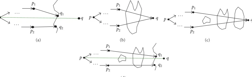
Figure 2: Construction of approximate optimal path between two points with obstacle constraints: (a) intersect with a linear obstacle; (b) intersect with the last planar obstacle; (c) intersect with a planar obstacle and obstacles behind it are all planar; (d) intersect with a planar obstacle and the obstacle behind it is linear.

Definition 1(linear obstacles). Let𝐿 = {𝐿_𝑖| 𝐿_𝑖= (𝑉_𝑖(𝐿), 𝐸(𝐿)_𝑖 ),

𝑖 ∈ 𝑍+_{} be polyline obstacles set, where𝑉}(𝐿)

𝑖 is the set of

vertices of𝐿_𝑖;𝐸_𝑖(𝐿) = {(V_𝑖𝑘,V_𝑖𝑘+1) | V_𝑖𝑘,V_𝑖𝑘+1 ∈ 𝑉_𝑖(𝐿),V_𝑖𝑘 is the adjacent vertex ofV_𝑖𝑘+1,𝑘 = 1, . . . , 𝑀_𝑖− 1, 𝑀_𝑖is the number of

𝑉_𝑖(𝐿)}.

Definition 2(planar obstacles). Let𝑆 = {𝑆_𝑖| 𝑆_𝑖 = (𝑉_𝑖(𝑆), 𝐸(𝑆)_𝑖 ),

𝑖 ∈ 𝑍+_{}be polygon obstacles set, where 𝑉}(𝑆)

𝑖 is the set of

vertices of𝑆_𝑖;𝐸(𝑆)_𝑖 = {(V_𝑖𝑘,V_{𝑖(𝑘+1)mod}

𝑁𝑖) | V𝑖𝑘,V𝑖(𝑘+1)mod_𝑁𝑖 ∈ 𝑉

(𝑆)

𝑖 ,

V_𝑖𝑘is the adjacent vertex ofV_𝑖(𝑘+1)

mod|𝑁𝑖|,𝑘 = 1, . . . , 𝑁𝑖, 𝑁𝑖is the

number of𝑉_𝑖(𝑆)}.

Definition 3(facilitators). Let𝑉_𝑐 = {𝑉_𝑖(𝐶) | 𝑉_𝑖(𝐶)is the set of

facilitators on the𝑖th obstacle}.

Definition 4(direct reachability). For any two points𝑝,𝑞in a

two-dimensional space,𝑝is called directly reachable from𝑞, if segment𝑝𝑞does not intersect with any obstacle; otherwise,

𝑝is called indirectly reachable from𝑞.

2.2. The Obstacle Distance between the Spatial Entities.

Cur-rently, the method of distance calculation often computes Euclidean distance between two clustering points. When physical obstacles exist in the real space, obstacles constraints should be taken into account to solve the distance between the two entities in the space. The algorithm handles linear obsta-cles and planar obstaobsta-cles, respectively. When traversing linear obstacles, facilitators are also taken into account for path construction. Figure2(a)illustrates the process of construct-ing approximate optimal path for linear obstacle, which presents a schematic view of Step 4 of the algorithm. When traversing planar obstacles, path is generated by the method to construct the minimum convex hull. In the case of no more than 100,000 two-dimensional space data samples, the calculation of the minimum convex hull can be finished within a few seconds [24]. Here Graham algorithm is used to produce the minimum convex hull [25]. Figures2(b)and

2(c)and Figure2(d), respectively, illustrate the construction process of the approximate optimal path for planar obstacles.

Figure2(b)shows a schematic view of the first case of Step 5. Figures2(c)and2(d)demonstrate a schematic view of the second case of Step 5.

For the sake of easy presentation of the path searching algorithm, the relevant symbols are defined as follows. Let

𝑜_𝑖∈ 𝐿∪𝑆be an obstacle, and𝑉_𝑖(𝑙)(󳨀→𝑝𝑞) ⊂ 𝑉_𝑐is the vertex subset

of𝑜_𝑖on your left hand when you walk along vector󳨀→𝑝𝑞from point𝑝to 𝑞. Similarly,𝑉_𝑖(𝑟)(󳨀→𝑝𝑞) ⊂ 𝑉_𝑐 is the vertex subset of𝑜_𝑖on the right hand.𝐺𝑟𝑎(𝑈, 𝑝, 𝑞) is the smallest convex hull which is constructed from the start point𝑝to the end point 𝑞 containing all the points of the vertex set 𝑈.

𝑃𝑎𝑡ℎ(𝑐)(𝐺𝑟𝑎(𝑈, 𝑝, 𝑞))denotes the path from the start point𝑝

to the end point 𝑞, which is constructed by the adja-cent edges of 𝐺𝑟𝑎(𝑈, 𝑝, 𝑞) in the clockwise direction;

𝑃𝑎𝑡ℎ(𝑐𝑐)_{(𝐺𝑟𝑎(𝑈, 𝑝, 𝑞))denotes the path from the start point𝑝}

to the end point𝑞, which is constructed by the adjacent edges

of𝐺𝑟𝑎(𝑈, 𝑝, 𝑞)in the counterclockwise direction.path1 and

path2, respectively, are the obstacle paths on the left and right hand of 󳨀→𝑝𝑞. When new segments are added to path1 and

path2, the start points of the added segments are denoted by

𝑝1and𝑝2, respectively. Similarly, the end points are denoted

by 𝑞1 and 𝑞2. 𝑑_𝑜(𝑝, 𝑞) represents the obstacle distance

between two spatial entities. If𝑝is directly reachablefrom

𝑞, 𝑑_𝑜(𝑝, 𝑞) is Euclidean distance between the two points,

denoted by𝑑(𝑝, 𝑞); if𝑝is indirectly reachablefrom𝑞, path is configured to bypass the obstacles while𝑝,𝑞, respectively, are taken as the start and end points.

The path searching algorithm for the approximate opti-mal path between two points among obstacles can be elabo-rated as follows.

Step 1. If 𝑝 is directly reachable from 𝑞, then 𝑑_𝑜(𝑝, 𝑞) =

𝑑(𝑝, 𝑞), and the algorithm is terminated; otherwise, go to Step

2.

Step 2. Find the obstacles intersect with󳨀→𝑝𝑞, which in turn are

represented as𝑜₁, 𝑜₂, . . . , 𝑜_𝑚 ∈ 𝐿 ∪ 𝑆, where𝑚is the number of the obstacles.

Step 3. Consider𝑝𝑎𝑡ℎ1 = 𝜙,𝑝𝑎𝑡ℎ2 = 𝜙,𝑝1 = 𝑝2 = 𝑝, and

Step 4. If𝑜_𝑖∈ 𝐿, execute the following steps.

(i) Select the vertex𝑢 ∈ 𝑉_𝑖(𝑙)(󳨀→𝑝𝑞)which has the smallest distance to󳨀→𝑝𝑞.

(ii) Select the vertexV∈ 𝑉_𝑖(𝑟)(󳨀→𝑝𝑞)which has the smallest distance to󳨀→𝑝𝑞.

(iii) Consider𝑞₁= 𝑢,𝑞₂ =V,𝑝𝑎𝑡ℎ1 = 𝑝𝑎𝑡ℎ1 ∪ 󳨀󳨀󳨀→𝑝₁𝑞₁, and

𝑝𝑎𝑡ℎ2 = 𝑝𝑎𝑡ℎ2 ∪ 󳨀󳨀󳨀→𝑝₂𝑞₂.

(iv) Consider𝑖 + +,𝑝₁= 𝑞₁, and𝑝₂= 𝑞₂.

(v) Go to Step 6.

Step 5. If𝑜_𝑖∈ 𝑆, there are the following two cases.

(I) If𝑖 == 𝑚, execute the following steps.

(i) If 𝑝󳨀󳨀→₁𝑞 intersects with 𝑜_𝑖, add𝑉_𝑖(𝑙)(󳨀󳨀→𝑝₁𝑞)to 𝑈₁,

𝑝𝑎𝑡ℎ1 = 𝑝𝑎𝑡ℎ1 ∪ 𝑃𝑎𝑡ℎ(𝑐)_{(𝐺𝑟𝑎(𝑈}

1, 𝑝1, 𝑞)).

(ii) If 𝑝󳨀󳨀→₂𝑞 intersects with 𝑜_𝑖, add 𝑉_𝑖(𝑟)(󳨀󳨀→𝑝₂𝑞)to 𝑈₂,

𝑝𝑎𝑡ℎ2 = 𝑝𝑎𝑡ℎ2 ∪ 𝑃𝑎𝑡ℎ(𝑐𝑐)_{(𝐺𝑟𝑎(𝑈}

2, 𝑝2, 𝑞)).

(iii) Consider𝑖 + +,𝑝₁= 𝑞, and𝑝₂= 𝑞. (iv) Go to Step 6.

(II) If𝑖 < 𝑚, execute the following steps.

(i) If 𝑜_𝑘(𝑘 = 𝑖, 𝑖 + 1, . . . , 𝑚) ∈ 𝑆, execute the following steps.

(a) Add 𝑉_𝑘(𝑙)(󳨀󳨀→𝑝₁𝑞)to 𝑈₁, 𝑝𝑎𝑡ℎ1 = 𝑝𝑎𝑡ℎ1 ∪

𝑃𝑎𝑡ℎ(𝑐)(𝐺𝑟𝑎(𝑈1, 𝑝1, 𝑞)).

(b) Add 𝑉_𝑘(𝑟)(󳨀󳨀→𝑝₂𝑞) to 𝑈₂, 𝑝𝑎𝑡ℎ2 = 𝑝𝑎𝑡ℎ2 ∪

𝑃𝑎𝑡ℎ(𝑐𝑐)_{(𝐺𝑟𝑎(𝑈}

2, 𝑝2, 𝑞)).

(c) Consider𝑖 = 𝑚,𝑝₁= 𝑞, and𝑝₂= 𝑞.

(ii) If𝑜_𝑖, 𝑜_𝑖+1, . . . , 𝑜_𝑘(𝑘 < 𝑚) ∈ 𝑆and 𝑜_𝑘+1 ∈ 𝐿, execute the following steps.

(a) Select the vertex𝑢 ∈ 𝑉_𝑘+1(𝑙)(󳨀→𝑝𝑞)which has the smallest distance to󳨀→𝑝𝑞.

(b) Select the vertexV ∈ 𝑉_𝑘+1(𝑟)(󳨀→𝑝𝑞) which has the smallest distance to󳨀→𝑝𝑞.

(c) Consider𝑞₁= 𝑢and𝑞₂=V.

(d) Add 𝑉_𝑖(𝑙)(󳨀󳨀󳨀→𝑝₁𝑞₁), 𝑉_𝑖+1(𝑙)(󳨀󳨀󳨀→𝑝₁𝑞₁), . . . , 𝑉_𝑘(𝑙)(󳨀󳨀󳨀→𝑝₁𝑞₁) to 𝑈₁. Consider 𝑝𝑎𝑡ℎ1 = 𝑝𝑎𝑡ℎ1 ∪

𝑃𝑎𝑡ℎ(𝑐)_{(𝐺𝑟𝑎(𝑈}

1, 𝑝1, 𝑞1)).

(e) Add 𝑉_𝑖(𝑟)(󳨀󳨀󳨀→𝑝₂𝑞₂), 𝑉_𝑖+1(𝑟)(󳨀󳨀󳨀→𝑝₂𝑞₂), . . . , 𝑉_𝑘(𝑟)(󳨀󳨀󳨀→𝑝₂𝑞₂) to 𝑈₂. Consider 𝑝𝑎𝑡ℎ2 = 𝑝𝑎𝑡ℎ2 ∪

𝑃𝑎𝑡ℎ(𝑐𝑐)_{(𝐺𝑟𝑎(𝑈}

2, 𝑝2, 𝑞2)).

(f) Consider𝑖 = 𝑘 + 1,𝑝₁= 𝑞₁, and𝑝₂= 𝑞₂.

Step 6. If𝑖 < 𝑚, go to Step 4; otherwise if𝑝₁! = 𝑞and𝑝₂! = 𝑞,

then𝑝𝑎𝑡ℎ1 = 𝑝𝑎𝑡ℎ1 ∪ 󳨀󳨀→𝑝₁𝑞,𝑝𝑎𝑡ℎ2 = 𝑝𝑎𝑡ℎ2 ∪ 󳨀󳨀→𝑝₂𝑞 ⋅ 𝑑_𝑜(𝑝, 𝑞) =

𝑚𝑖𝑛(𝑙𝑒𝑛𝑔𝑡ℎ(𝑝𝑎𝑡ℎ1), 𝑙𝑒𝑛𝑔𝑡ℎ(𝑝𝑎𝑡ℎ2)).

2.3. Spatial Clustering Algorithm with Obstacle Constraints

Based on Artificial Immune System. Computational

intelli-gence techniques have been widely applied to data engineer-ing research, includengineer-ing classification, clusterengineer-ing, deviation, or outlier detection [19]. Artificial immune system (AIS) is an intelligent method, which mimics natural biological function of the immune system. For its promising performance in immune recognition, the ability of immune learning and immune memory, AIS gradually becomes an important branch of intelligent computing [26–29]. In order to solve the problems of the traditional cluster algorithm in sensitivity to the initial value and the tendency to fall into local optimum, while maintaining its advantages of fast convergence speed, a novel spatial clustering algorithm with obstacle constraints is proposed in this paper.

2.3.1. The Clustering Problem. Given𝑉, the goal of a

cluster-ing algorithm is to obtain a partition𝐼 = {𝐼₁, 𝐼₂, . . . , 𝐼_𝑘}(i.e.,

𝐼𝑖 ̸= 𝜙, for all𝑖;⋃𝑘𝑖=1𝐼𝑖 = 𝑉;𝐼𝑖∩ 𝐼𝑗 = 𝜙, for all𝑖 ̸= 𝑗) which

satisfies that objects classified as the same cluster are as similar to each other as possible, whereas objects classified as the different clusters are as dissimilar as possible.

2.3.2. Antibody Encoding. Let𝑉 = {V₁,V₂, . . . ,V_𝑀}be a set

of𝑀sample points, corresponding to the antigen set𝐴𝑔𝑠 =

{𝑎𝑔₁, 𝑎𝑔₂, . . . , 𝑎𝑔_𝑀}. The antibody set 𝐴𝑏𝑠 = {𝑎𝑏₁, 𝑎𝑏₂, . . . ,

𝑎𝑏_𝑁}, where𝑁is the number of antibodies. Each antibody𝑎𝑏_𝑖 consists of𝑘cluster centers, and each cluster center can be expressed as a real-value𝑑-dimensional profile vector which is represented as 𝑎𝑏_𝑖 = {𝑎_{⏟⏟⏟⏟⏟⏟⏟⏟⏟⏟⏟⏟⏟⏟⏟⏟⏟⏟⏟⏟⏟⏟⏟11}𝑎₁₂. . . 𝑎_1𝑑

𝑐1 ⋅ ⋅ ⋅ 𝑎⏟⏟⏟⏟⏟⏟⏟⏟⏟⏟⏟⏟⏟⏟⏟⏟⏟⏟⏟⏟⏟𝑖1𝑎𝑖2𝑐𝑖. . . 𝑎𝑖𝑑⋅ ⋅ ⋅

𝑎_𝑘1𝑎_𝑘2. . . 𝑎_𝑘𝑑

⏟⏟⏟⏟⏟⏟⏟⏟⏟⏟⏟⏟⏟⏟⏟⏟⏟⏟⏟⏟⏟⏟⏟ 𝑐𝑘

}, where𝑐_𝑖corresponds to the center of the𝑖

th-cluster.

2.3.3. Affinity Function Design and Immune Operators. In

most occasions, the most used similarity metric in a clus-tering algorithm is distance metric. The total within-cluster variance or the total mean-square quantization error (MSE) [30] is calculated as follows:

Perf(𝑉, 𝐶) =

𝑚 ∑

𝑖=1{󵄩󵄩󵄩󵄩󵄩

V_𝑖− 𝑐𝑗󵄩󵄩󵄩󵄩_󵄩2, 𝑗 = 1, . . . , 𝑘} , (1)

where‖V_𝑖− 𝑐_𝑗‖denotes the similarity between sample point

V_𝑖and clustering center𝑐_𝑗and the obstacle distance is used as a distance metric in this paper. Obstacles constraints should be taken into account for clustering algorithms in the paper. On this basis, cluster centers set𝐶 = {𝑐₁, 𝑐₂, . . . , 𝑐_𝑘}and the corresponding partition𝐼 = {𝐼₁, 𝐼₂, . . . , 𝐼_𝑘}are achieved by applying the rule that the nearer sample points are apart from a cluster center in obstacle distance.

Bearing in mind the measurement of the MSE in (1), we design an affinity function𝑓_𝑖,𝑗in (2), which represents the affinity of the antibody of𝑖with antigen𝑗. Let𝐷in-cluster =

∑𝑘_𝑗=1∑_{V𝑖∈𝑉∩𝐼𝑗}𝑑_𝑜(V_𝑖, 𝑐_𝑗); then

𝑓_𝑖,𝑗= 1

where 𝜀₀ is a small positive number to avoid illness (i.e., denominator equals zero).fmeansdenotes the average value of population affinity, which can be calculated as

𝑓𝑚𝑒𝑎𝑛𝑠 = ∑

𝑘

𝑖=1∑𝑚𝑗=1𝑓𝑖,𝑗

𝑘 . (3)

𝑀 ⊆ 𝐴𝑏𝑠is memory cell subset. Threshold value of

immuno-suppression is calculated as

𝛼 = _𝑘1₂𝑘−1∑

𝑖=1 𝑘 ∑ 𝑗=𝑖+1

𝑓_𝑖,𝑗󸀠, (4)

where 𝑓_𝑖,𝑗󸀠 = 𝑑_𝑜(𝑐_𝑖, 𝑐_𝑗), which represents the affinity of the antibody of𝑖with antibody𝑗.

The antibody selection operations, cloning operations, and mutation operations of AICOE algorithm were defined in the literature [31].

2.3.4. Artificial Immune Clustering with Obstacle Entity

(AICOE) Algorithm. F 𝐴𝑔𝑠 = {𝑎𝑔₁, 𝑎𝑔₂, . . . , 𝑎𝑔_𝑀}, the

algorithm is described as follows.

Step 1. Initialize antibody set 𝐴𝑏𝑠(0) = {𝑎𝑏₁, 𝑎𝑏₂, . . . , 𝑎𝑏_𝑁},

where𝑁is the number of antibodies. Consider𝑡 = 0.

Step 2. For all𝑎𝑔_𝑖∈ 𝐼_𝑘(1 ≤ 𝑖 ≤ 𝑀, 1 ≤ 𝑘 ≤ 𝑁), calculate the

value of𝑓_𝑖,𝑘according to (2).

Step 3. According to the affinity calculations by Step 2,

opti-mal antibody subset𝑏𝑠𝑡𝐴𝑆is composed of top𝐾(𝐾 ≤ 𝑁) affinity antibodies where𝑏𝑠𝑡𝐴𝑆 ⊆ 𝐴𝑏𝑠(𝑡). Add𝑏𝑠𝑡𝐴𝑆to𝑀.

Step 4. Generation of the next generation antibody set is

elaborated as follows.

(I) Obtain bstAS1 via performing clone operation on

bstAS.

(II) ObtainbstAS2 via performing mutation operation on

bstAS1. AddbstAS2 to𝑀.

(III) Implement the immunosuppression operation on𝑀. Calculate the value of𝛼according to (4). For all𝑎𝑏_𝑖,

𝑎𝑏𝑖 ∈ 𝑀, if the value of𝑓𝑖,𝑗󸀠 is less than𝛼, randomly

delete one of the two antibodies.

(IV) Randomly generate antibody subset to update the next generation antibody set, denoted byrdmAS. (V) Add𝑀and𝑟𝑑𝑚𝐴𝑆to𝐴𝑏𝑠(𝑡 + 1). Consider𝑡 = 𝑡 + 1.

Step 5. Calculate the value of thefmeans of contemporary

population by using (3). If the differencefmeansin certain continual iterations does not exceed 𝜀, stop the algorithm; otherwise go to Step 2.

3. Case Implementation and Results

This paper presents two sets of experiments to prove the effectiveness of the AICOE algorithm. The first experiment

uses a set of simulated data, which are generated by the simulation of ArcGIS 9.3. Experimental results are compared with𝐾-means clustering algorithm [2,3]. The second exper-iment is carried out on a case study on Wuhu city and compares the results with the COE-CLARANS algorithm [8]. All algorithms are implemented in C# language and executed

onPentium4.3 HZ, 2 GB RAM computers. The main

param-eters of the algorithm are defined as follows: mutation rate

𝑝_𝑚 = 0.35, inhibition threshold𝛼 = 0.05, and the iterative

stopping criteria parameter𝜀 = 1.0𝑒 − 4.

3.1. Simulation Experimental Results. The classical𝐾-means

clustering algorithm has been widely used for its simplicity and feasibility. The AICOE algorithm uses obstacle distance defined in this paper for clustering analysis, and𝐾-means algorithm uses Euclidean distance as similarity measure of samples. Simulated dataset of the first experiment is shown in Figure3(a). When cluster number𝑘 = 6, the clustering results of𝐾-means clustering algorithm and AICOE algorithm are shown in Figures3(b)and 3(c), respectively. Experimental results show that the clustering results of the AICOE algo-rithm considering obstacles and facilitators are more efficient than𝐾-means algorithm.

3.2. A Case Study on Wuhu City

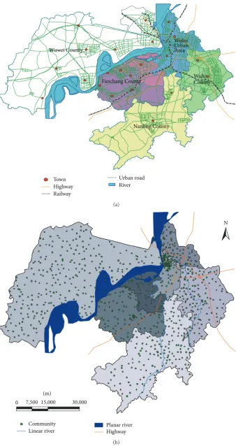
3.2.1. Study Area and Data. In this test, the AICOE

algo-rithm is applied to an urban spatial dataset of the city of Wuhu in China (Figure4). This paper takes 994 residential communities as two-dimensional points, where the points are represented as(𝑥, 𝑦). In this case study, each residential community is treated as cluster sample point, with its popu-lation being an attribute. The highways, rivers, and lakes in the territory are regarded as spatial obstacles, as defined in Definitions1and2, respectively. Pedestrian bridge and under-pass on a highway and the bridge on the water body serve as connected points, and the remaining vertices are uncon-nected points. Digital map of Chinese Wuhu stored in ArcGis 9.3 was used. And automatic programming has been devised to generate spatial points as cluster points to the address of the residential communities. The purpose of this paper is to find the suitable centers (medoids) and their corresponding clusters.

3.2.2. Clustering Algorithm Application and Contrastive

Anal-ysis. The COE-CLARANS algorithm [8] and the AICOE

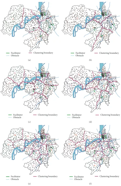
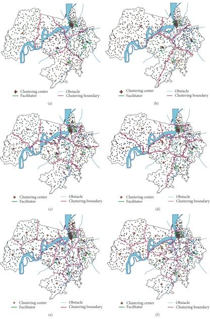
algorithm are compared by simulation experiment. The AICOE algorithm uses obstacle distance defined in this paper for clustering analysis. The comparison results of clustering analysis using COE-CLARANS algorithm and AICOE algo-rithm are shown in Figure 5, and the comparison results of clustering analysis using COE-CLARANS algorithm and AICOE algorithm considering clustering centers are shown in Figure6.

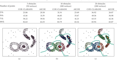
Table 1: Run time comparison of COE-CLARANS and AICOE (seconds).

Number of points

5 obstacles (50 vertices)

10 obstacles (100 vertices)

20 obstacles (200 vertices)

COE-CLARANS AICOE COE-CLARANS AICOE COE-CLARANS AICOE

25 k 25.86 20.58 31.54 25.69 36.92 26.87

50 k 43.16 31.59 46.85 35.67 49.36 36.98

75 k 58.22 39.56 61.23 41.23 63.33 42.36

100 k 82.63 64.55 83.79 65.32 83.94 65.87

(a) (b) (c)

Figure 3: Clustering spatial points in the presence of obstacles and facilitators: (a) simulated dataset; (b) clustering results of𝐾-means algorithm with obstacles and facilitators; (c) clustering results of AICOE algorithm with obstacles and facilitators.

clustering result of its surrounding regions can demonstrate the validity of the algorithm. Setting cluster number𝑘 = 5, the clustering results of the AICOE algorithm show that only one clustered region 2 has been passed through by Yangtze River where Wuhu Yangtze River Bridge plays a role as a facilitator. While the clustering results of the COE-CLARANS algorithm show that Yangtze River has passed through two clusters, the clustered region 2 does not have any facilitators. Setting cluster number𝑘 = 10, the clustering results of the COE-CLARANS algorithm show that Yangtze River has passed through three subclass regions and the clustered regions 3 and 4 do not have any facilitators. Setting cluster number𝑘 = 15, there does not exist any facilitator in the clustered region 11 obtained by the COE-CLARANS algorithm. In comparison, the clustering results of the AICOE algorithm show that only one clustering region has been passed through by Yangtze River where the facilitator exists. The simulation results demonstrate that the impacts of obstacles on clustering results correspondingly reduce along with the increase in the number of cluster regions.

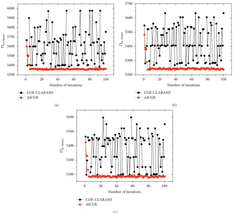
Figure 7 demonstrates that the COE-CLARANS algo-rithm is sensitive to initial value, while the AICOE algoalgo-rithm avoids this flaw effectively. Meanwhile, the AICOE algorithm can get global optimal solution in fewer iterations.

Table 1shows the results of scalability experiments for the comparison of the COE-CLARANS algorithm and the AICOE algorithm. The synthetic dataset in the following experiments is generated from a Gaussian distribution. The size of dataset varies from 25,000 to 100,000 points. The obstacles and facilitators are generated manually. The number of the obstacles varies from 5 to 20, and the number of vertices

of each obstacle is 10. The number of the facilitators accounts for 20% of the number of the obstacles. Table 1illustrates that the AICOE algorithm is faster than the COE-CLARANS algorithm.

By comparison of the COE-CLARANS algorithm and the AICOE algorithm for handling spatial clustering with physi-cal constraints, the experimental results show that the COE-CLARANS algorithm causes grouping biases due to its micro-clustering approach. Correspondingly, the AICOE algorithm operates with all the data with less prior preprocessing. The quality of clustering results achieved by the AICOE algorithm surpasses the results of the COE-CLARANS algorithm. Next, the simulation results also indicate that the AICOE algorithm overcomes the COE-CLARANS shortcoming of sensitivity to initial value. The reason for this drawback is that COE-CLARANS algorithm selects the optimum set of represen-tatives for clusters with a two-phase heuristic method. Last, the results of scalability experiments illuminate that the COE-CLARANS algorithm which is affected by the low efficiency of preprocessing runs slower than the AICOE algorithm.

4. Conclusions

Town Highway Railway

Urban road River

Nanling County Wuwei County

Fanchang County WuhuCounty

Wuhu Urban Area

(a)

Community Linear river

Planar river Highway 0 7,500 15,000 30,000

N

(m)

(b)

Facilitator Obstacle

Clustering boundary 5

4 3 2

1

(a)

Facilitator Obstacle

Clustering boundary 5

4

3 2

1

(b)

Facilitator Obstacle

Clustering boundary 10

9

8

7 6

5 4

3 2

1

(c)

Facilitator Obstacle

Clustering boundary 10 9

8 7

6 5

4

3 2

1

(d)

14

15 ₁₃

12 11 10

9 8

7 6

5 ₄

3 2

1

Facilitator Obstacle

Clustering boundary

(e)

Facilitator Obstacle

Clustering boundary 1

3 4 11

6

8

7 2

9 10

12 13

14 15

5

(f)

Clustering center Facilitator

Obstacle

Clustering boundary

(a)

Clustering center Facilitator

Obstacle

Clustering boundary

(b)

Clustering center Facilitator

Obstacle

Clustering boundary

(c)

Clustering center Facilitator

Obstacle

Clustering boundary

(d)

Clustering center Facilitator

Obstacle

Clustering boundary

(e)

Clustering center Facilitator

Obstacle

Clustering boundary

(f)

0 20 40 60 80 100

AICOE COE-CLARANS

Number of iterations 5300

5400 5500 5600 5700 5800 5900 6000

Din-c

lu

st

er

(a)

0 20 40 60 80 100

AICOE COE-CLARANS

Number of iterations 5200

5300 5400 5500 5600 5700

Din-c

lu

st

er

(b)

0 20 40 60 80 100

AICOE COE-CLARANS

Number of iterations 5200

5300 5400 5500 5600

Din-c

lu

st

er

(c)

Figure 7: Comparison of clustering analysis using the COE-CLARANS algorithm and the AICOE algorithm by intercluster distances: (a) cluster number𝑘 = 5; (b) cluster number𝑘 = 10; (c) cluster number𝑘 = 15.

metric into affinity function calculation of immune clonal optimization and updating the cluster centers based on the elite antibodies, the AICOE algorithm effectively solves the shortcomings of the traditional method. The comparative experimental and case study with the classic clustering algorithms has demonstrated the rationality, performance, and practical applicability of the AICOE algorithm.

Due to the complexity of geographic data and the differ-ence of data formats, present researches on spatial clustering with obstacle constraint mainly aim at clustering method for two-dimensional spatial data points [8,10,12–14]. There are two directions for future work. One is to extend our approach for conducting comprehensive experiments on more complex databases from real application. The other is to take nonspa-tial attributes into account for a comprehensive analysis of spatial database.

Conflict of Interests

The authors declare that there is no conflict of interests regarding the publication of this paper.

Acknowledgments

This work is supported by the National Natural Science Foundation of China under Grant no. 61370050 and the Nat-ural Science Foundation of Anhui Province under Grant no. 1308085QF118.

References

[2] J. Macqueen, “Some method for classification and analysis of multivariate observations,” inProceedings of the 5th Berkeley Symposium on Mathematical Statistics and Probability, pp. 281– 297, 1967.

[3] L. Kaufman and P. Rousseeuw, Finding Groups in Data: An Introduction to Cluster Analysis, John Wiley & Sons, New York, NY, USA, 1990.

[4] T. Zhang, R. Ramakrishnan, and M. Livny, “BIRCH: an efficient data clustering method for very large databases,” inProceedings of the ACM SIGMOD International Conference on Management of Data, pp. 103–114, Montreal, Canada, 1996.

[5] S. Guha, R. Rastogi, and K. Shim, “CURE: an efficient clustering algorithm for large databases,” in Proceedings of the ACM SIGMOD International Conference on Management of Data, vol. 27, pp. 73–84, 1998.

[6] J. Sander, M. Ester, H.-P. Kriegel, and X. Xu, “Density-based clustering in spatial databases: the algorithm GDBSCAN and its applications,”Data Mining and Knowledge Discovery, vol. 2, no. 2, pp. 169–194, 1998.

[7] X. Wang, C. Rostoker, and H. Hamilton, “Density-based spatial clustering in the presence of obstacles and facilitators,” in Proceedings of the 8th Pacific-Asia Conference on Knowledge Discovery and Data Mining, pp. 446–458, 2004.

[8] A. Tung, J. Hou, and J. Han, “COE: clustering with obstacles entities, a preliminary study,” inProceedings of the 4th Pacific-Asia Conference on Knowledge Discovery and Data Mining, pp. 165–168, 2000.

[9] R. Ng and J. Han, “Efficient and effective clustering methods for spatial data mining,” inProceedings of the 20th Conference on Very Large Databases, pp. 144–155, Santiago, Chile, 1994. [10] O. R. Za¨ıane and C.-H. Lee, “Clustering spatial data when

facing physical constraints,” in Proceedings of the 2nd IEEE International Conference on Data Mining (ICDM ’02), pp. 737– 740, IEEE, December 2002.

[11] M. Ester, H. Kriegel, J. Sander, and X. Xu, “A density-based algorithm for discovering clusters in large spatial databases with noise,” inProceedings of the 2nd International Conference on Knowledge Discovery and Data Mining, pp. 226–231, 1996. [12] X. Wang, C. Rostoker, and H. J. Hamilton, “A density-based

spatial clustering for physical constraints,”Journal of Intelligent Information Systems, vol. 38, no. 1, pp. 269–297, 2012.

[13] V. Estivill-Castro and I. Lee, “Clustering with obstacles for Geographical Data Mining,”ISPRS Journal of Photogrammetry and Remote Sensing, vol. 59, no. 1-2, pp. 21–34, 2004.

[14] Q. Liu, M. Deng, and Y. Shi, “Adaptive spatial clustering in the presence of obstacles and facilitators,” Computers and Geosciences, vol. 56, pp. 104–118, 2013.

[15] W. Ma, L. Jiao, and M. Gong, “Immunodominance and clonal selection inspired multiobjective clustering,”Progress in Natural Science, vol. 19, no. 6, pp. 751–758, 2009.

[16] A. Graaff and A. Engelbrecht, “Clustering data in an uncertain environment using an artificial immune system,”Pattern Recog-nition Letters, vol. 32, no. 2, pp. 342–351, 2011.

[17] C.-Y. Chiu, I.-T. Kuo, and C.-H. Lin, “Applying artificial immune system and ant algorithm in air-conditioner market segmenta-tion,”Expert Systems with Applications, vol. 36, no. 3, pp. 4437– 4442, 2009.

[18] W. Huang and L. Jiao, “Artificial immune kernel clustering net-work for unsupervised image segmentation,”Progress in Natural Science, vol. 18, no. 4, pp. 455–461, 2008.

[19] Q. Cai, H. He, and H. Man, “Spatial outlier detection based on iterative self-organizing learning model,”Neurocomputing, vol. 117, pp. 161–172, 2013.

[20] A. J. Graaff and A. P. Engelbrecht, “Using sequential deviation to dynamically determine the number of clusters found by a local network neighbourhood artificial immune system,”Applied Soft Computing Journal, vol. 11, no. 2, pp. 2698–2713, 2011.

[21] M. Bereta and T. Burczy´nski, “Immune𝐾-means and negative selection algorithms for data analysis,”Information Sciences, vol. 179, no. 10, pp. 1407–1425, 2009.

[22] S. Gou, X. Zhuang, Y. Li, C. Xu, and L. C. Jiao, “Multi-elitist immune clonal quantum clustering algorithm,” Neurocomput-ing, vol. 101, pp. 275–289, 2013.

[23] R. Liu, X. Zhang, N. Yang, Q. Lei, and L. Jiao, “Immunodoma-ince based clonal selection clustering algorithm,”Applied Soft Computing, vol. 12, no. 1, pp. 302–312, 2012.

[24] J. Wang, “Study of optimizing method for algorithm of mini-mum convex closure building for 2D spatial data,”Acta Geo-daetica et Cartographica Sinica, vol. 31, no. 1, pp. 82–86, 2002. [25] R. L. Graham, “An efficient algorithm for determining the

convex hull of a finite planar set,”Information Processing Letters, vol. 1, no. 4, pp. 132–133, 1972.

[26] A. Diabat, D. Kannan, M. Kaliyan, and D. Svetinovic, “A opti-mization model for product returns using genetic algorithms and artificial immune system,” Resources, Conservation and Recycling, vol. 74, pp. 156–169, 2013.

[27] O. Er, N. Yumusak, and F. Temurtas, “Diagnosis of chest diseases using artificial immune system,”Expert Systems with Applications, vol. 39, no. 2, pp. 1862–1868, 2012.

[28] M. Basu, “Artificial immune system for dynamic economic dispatch,”International Journal of Electrical Power & Energy Systems, vol. 33, no. 1, pp. 131–136, 2011.

[29] M. M. El-Sherbiny and R. M. Alhamali, “A hybrid particle swarm algorithm with artificial immune learning for solving the fixed charge transportation problem,”Computers and Industrial Engineering, vol. 64, no. 2, pp. 610–620, 2013.

[30] Z. G¨ung¨or and A. ¨Unler, “𝐾-harmonic means data clustering with simulated annealing heuristic,”Applied Mathematics and Computation, vol. 184, no. 2, pp. 199–209, 2007.

Submit your manuscripts at

http://www.hindawi.com

Computer Games Technology

International Journal of

Hindawi Publishing Corporation

http://www.hindawi.com Volume 2014

Hindawi Publishing Corporation

http://www.hindawi.com Volume 2014

Distributed Sensor Networks

International Journal of

Advances in

Fuzzy

Systems

Hindawi Publishing Corporation

http://www.hindawi.com Volume 2014

International Journal of

Reconfigurable Computing

Hindawi Publishing Corporation

http://www.hindawi.com Volume 2014

Hindawi Publishing Corporation

http://www.hindawi.com Volume 2014

Applied

Computational

Intelligence and Soft

Computing

 Advances in 

Artificial

Intelligence

http://www.hindawi.com Volume 2014

Advances in

Software Engineering

Hindawi Publishing Corporation

http://www.hindawi.com Volume 2014

Hindawi Publishing Corporation

http://www.hindawi.com Volume 2014 Electrical and Computer Engineering

Journal of

Journal of

Computer Networks and Communications

Hindawi Publishing Corporation

http://www.hindawi.com Volume 2014 Hindawi Publishing Corporation

http://www.hindawi.com Volume 2014

Multimedia

International Journal of

Biomedical Imaging

Hindawi Publishing Corporation

http://www.hindawi.com Volume 2014

Artificial

Neural Systems

Advances in

Hindawi Publishing Corporation

http://www.hindawi.com Volume 2014

Robotics

Hindawi Publishing Corporation

http://www.hindawi.com Volume 2014 Hindawi Publishing Corporationhttp://www.hindawi.com Volume 2014 Computational Intelligence and Neuroscience

Hindawi Publishing Corporation

http://www.hindawi.com Volume 2014

Modelling & Simulation in Engineering

Hindawi Publishing Corporation

http://www.hindawi.com Volume 2014

The Scientific

World Journal

Hindawi Publishing Corporation

http://www.hindawi.com Volume 2014

Hindawi Publishing Corporation

http://www.hindawi.com Volume 2014

Human-Computer Interaction Advances in

Computer EngineeringAdvances in

Hindawi Publishing Corporation