Policy evaluation via a statistical control: A non-parametric evaluation of the 'Want2Work' active labour market policy

(1)

Policy evaluation via a statistical control: A non-parametric evaluation of

the

‘

Want2Work

’

active labour market policy

Joanne Lindley

a

, Steven Mcintosh

b

, Jennifer Roberts

b,

⁎

, Carolyn Czoski Murray

c

, Richard Edlin

d a_{Department of Management, King's College London, Franklin–Wilkins Building, 150 Stamford Street, London SE1 9NH, UK}

b_{Department of Economics, University of Shef}_ﬁ_{eld, 9 Mappin Street, Shef}_ﬁ_{eld S1 4DT, UK} c

Leeds Institute of Health Sciences, Charles Thackrah Building, 101 Clarendon Road, Leeds LS2 9LJ, UK d

Faculty of Medical and Health Sciences, University of Auckland, New Zealand

a b s t r a c t

a r t i c l e i n f o

Article history:

Accepted 12 September 2015 Available online 3 October 2015

Keywords:

Active labour market policy Statistical control Propensity score matching

Active labour market policies are popular tools used by governments to help get unemployed people back into work. It is a common problem that interventions of this type are often established with no equivalent control group on which to base an evaluation of programme effectiveness. This study uses propensity score matching to evaluate the success of an active labour market policy (the Welsh Assembly's‘Want2Work’programme) that cannot otherwise be evaluated using standard parametric techniques. Using a range of matching and estima-tion methods, sub-samples and types of job, the scheme was successful. Our most conservative estimate indicates that participants were 7 percentage points more likely tofind employment than a control group of non-treated job-seekers. The method adopted here is a useful addition to the real world policy evaluation tool kit, where programme effectiveness needs to be judged in the absence of an established control group. Our results provide evidence that even those who are currently out of the labour market and on health related benefits canfind work with the help of appropriately designed support.

1. Introduction

The Want2Work (W2W) scheme was an active labour market policy that was introduced by the Welsh Assembly Government in the UK in order to improve the chances of individuals currently out of work re-entering the labour market. Active labour market policies have become increasingly popular and seem particularly attractive to governments in times of recession (Martin, 2015). This paper evaluates the W2W pilot scheme, which ran from September 2004 until March 2008 in particular areas of Wales.1The primary aim of the scheme was to improve the re-employment chances of the participants.

W2W was aimed at Incapacity Beneﬁt (IB) recipients; IB is a beneﬁt for people who are unable to work due to health problems. Hence, many of the key features of the scheme were concerned with the health status of participants. The scheme was voluntary and advertisements detailing the services on offer were placed in public places such as doctors' surgeries.2

The key features of the programme include a combination of mea-sures aimed at improving the information of participants as well as

providingﬁnancial incentives. In terms of information provision, a net-work of community-based advisers was appointed to provide advice and guidance. In addition, a health professional was attached to each team to support these advisors, to develop links to local health services, and to provide information to participants as to how they could cope with their health problems in order to participate in the labour market. Participants also received in-work development and support during the ﬁrst year of employment.

In terms offinancial incentives, a return to work bursary was provided, consisting of a weekly payment to individuals to cover the costs of returning to work. This paid £60 per week during thefirst four months in work, £40 per week in the second four months and £20 per week in the third four-month period of thefirst year in work. There was also pro-vision of, or funding for, training, including the development of‘soft’skills (such as time management and communication), as well as a job prepara-tion premium, paid to participants to cover the cost of undertaking addi-tional work preparation activities. Finally there was discretionary funding available to overcome other barriers to participation in employment.

The aim of this paper is to determine whether all of these additional services,3_{over and above standard assistance to those out of work, led} ⁎ Corresponding author.

E-mail address:j.r.roberts@shefﬁeld.ac.uk(J. Roberts).

1_{The selected areas for the W2W pilots were selected wards within the Cardiff, Neath} Port Talbot, Merthyr Tydﬁl, Caerdigion and Denbighshire unitary authority areas.

2

As advertisements were also placed in local job centres, non-IB claimants wanted to be involved, and the scheme was expanded to include all those out of work. Nevertheless, it retained its focus on IB-claimants.

3

Unfortunately, the available data did not allow us to study the various aspects of the programme separately, to determine which aspects of the scheme were most successful in terms of getting people into work. In particular we are not able to distinguish between ﬁnancial and non-ﬁnancial incentives.

http://dx.doi.org/10.1016/j.econmod.2015.09.018

Economic Modelling

(2)

to an increase in the likelihood that participants obtained a job. The chal-lenge to be faced is common for such policy evaluations: Would the successful participants still have obtained a job even if they had not par-ticipated in the W2W scheme? An additional issue here is common to many public programmes; a control group was not established as part of the original evaluation protocol and participation in the scheme was voluntary. To deal with these problems we use propensity score matching (PSM) techniques to derive a statistical control group of non-participants with similar observed characteristics to those who participate in W2W, and then compare the employment probabilities of each group. Unlike parametric methods used for previous similar policy evaluations, PSM does not impose any particular functional form on the estimated relation-ships. PSM was used for example byBrown and Taylor (2011)in their analysis of the divergence between the reservation wages of individuals who are out of work and their predicted market wages. The next section reviews some other recent evaluations of active labour market policies in the UK. The following section then describes the data and methodology to be used, followed by a presentation of the results. Aﬁnal section offers a summary and some conclusions.

2. Recent evaluations of active labour market policies in the UK

In the last decade or so, a number of large-scale active labour market policies have been introduced in the UK. The scheme most similar to W2W, in terms of a focus on IB individuals, is Pathways to Work (Path-ways). This was introduced, initially on a pilot basis in three local areas, in October 2003, and ran until 2011. Pathways was compulsory for all new IB claimants and was available on a voluntary basis for existing claimants. Many of the elements were similar to the W2W programme. Various evaluations of Pathways have been undertaken.Adam et al. (2006)used a difference-in-differences (DiD) technique to compare the difference in the re-employment rates between pilot and non-pilot areas before and after the introduction of Pathways. The results show that, amongst those beginning a claim for IB, Pathways increased the percentage in employment 101/2months later by an estimated 9.4 per-centage points, from a base of just 22.5%.Bewley et al. (2007) consid-ered a longer time period, ﬁnding that Pathways increased the probability of an initial IB claimant being in work eighteen months later by 7.4 percentage points, from a base of 29.7% in the absence of the policy.

Bewley et al. (2008)also considered the impact of Pathways on existing IB claimants. A policy variation was introduced in February 2005 in that individuals living in the pilot areas with an IB claim of up to 2 years when Pathways wasﬁrst introduced were also required to participate in the scheme. Using a duration analysis approach, becoming involved in Pathways reduced the probability of still being out of work by 3.5 percentage points eighteen months later, from 97.2% to 93.7%. Thus, the impact of the programme was signiﬁcantly reduced when applied to those who were in the middle of an IB claim, rather than to those at the start of their claim.

A second active labour market scheme that has attracted a lot of at-tention is the New Deal, and in particular the New Deal for Young People (NDYP). This scheme was piloted in selected areas of the UK in January 1998 and rolled-out nationally in April 1998. NDYP is a compulsory scheme for young people aged 18–24 who have been out of work for 6 months. The scheme involves an initial‘Gateway’period of around 4 months, where extensive job search help is provided. If the participant fails to obtain a job in this period, they can spend up to one year in one of four options provided by NDYP: a period of education and train-ing; a subsidised job; a job in the voluntary sector; or work with an en-vironmental task force.

Again, a number of evaluations of NDYP have been undertaken.

Blundell et al. (2004)conducted a DiD analysis, where the control group consisted of individuals with similar observed characteristics in non-pilot areas during the pilot phase, or individuals with similar ob-served characteristics and living in the same area, but aged just over

24 and so not eligible for NDYP, in the roll-out phase. The authors only studied the impact of the initial four month Gateway period, and found that in the former (pilot versus non-pilot) case, participating in the Gateway increased male individuals' prospects of having moved into employment four months after joining the Gateway by 10–11 per-centage points, from a base of 24%. When they studied the national roll-out using the older comparison group, the impact fell to 5 percentage points, against a base of 26%. They attributed the fall in the size of the ef-fect to the maturing of the scheme, and the loss of the‘program intro-duction effect’. Also using this second method, but considering a longer time period,De Giorgi (2005)found that NDYP participation in-creased the male re-employment probability after eighteen months by 4.6 percentage points, thus very similar to the estimate obtained by

Blundell et al. (2004). There was no evidence of the NDYP effect falling further over time, as the programme matured.

Other papers have evaluated NDYP in more detail, looking at varia-tions in the average effect. A good example isMcVicar and Podivinsky (2009)who considered whether the impact of NDYP varies across re-gions and in particular with the tightness of their labour markets. They used a DiD approach to duration analysis, comparing the change in unemployment durations for 18–24 years olds before and after the introduction of NDYP, to the similar before and after changes for 25–29 year olds who form the control group. Their results show that NDYP reduced unemployment durations for young men in all regions, with the size of the effect being positively, though weakly, related to local unemployment rates, so that NDYP had a greater impact in slack labour markets.

The evaluation methodology to be used in this paper is PSM.Dorsett (2001)used this approach to evaluate NDYP. All four post-Gateway op-tions were considered, and in each case the control group compromised those individuals who followed one of the‘other’three options, as well as those young people who remain on the Gateway longer than the four month period without entering any of the options. For each pairwise combination of options in turn, PSM was used to match individuals fol-lowing one option, to a similar person folfol-lowing the other. The results showed that the subsidised employment option dominated all others in reducing the likelihood of remaining unemployed.

3. Data and methodology

The key to a good programme evaluation is successfully estimating the counterfactual, of what would have happened to the participants if they had not engaged in the programme. Given that we cannot observe participants in the non-participation state at the same point in time as they are participating, then data on non-participants must be used to estimate the counterfactual. It is therefore important that there is good information available on both the treatment and control groups (participants and non-participants), so that any differences in charac-teristics, which may in turn have explained differences in employment outcomes, are held constant.

Extensive data on W2W participants was collected at their point of entry to the scheme.4_{Any future changes in status, such as a movement} into employment or training, were also recorded. Anyone who joined W2W between January 2005 and December 2007 is included, so we have information on the full population of W2W participants between these dates (approximately 6400 individuals).5_{The W2W database} con-tains detailed information on background characteristics, including age, gender, ethnicity, whether a single parent or not, highest qualification, type of welfare benefit being received when first registered with W2W, type of any illness or disability, and time spent out of work. This latter is a particularly useful control variable in that it will proxy

4 _{The database of information on W2W participants was collected by the Welsh} Assem-bly Government.

5

(3)

for unobserved‘employability’characteristics. If the individualﬁnds a job during the observation period, then some characteristics of that job are also recorded, such as annual earnings, full- or part-time status and permanent or temporary status, as well as the date that the job started.

The counterfactual data used for the control group are drawn from the Quarterly Labour Force Survey (QLFS) for Great Britain.6_{The QLFS} has a wealth of information on employment outcomes and job charac-teristics, as well as all of the individual level characteristics that are ob-served for the W2W participants. Each quarter's sample of the QLFS has 60,000 private households made up of 5‘cohorts’, each in different re-sponse‘waves’. Therefore, in any one quarterly survey, one-fifth of re-spondents are participating for thefirst time, one-fifth for the second time, etc., with one-fifth being replaced each quarter. The QLFS is there-fore a rolling panel where each cohort is interviewed in 5 successive quarters.

Since the W2W data cover the period 2005 to 2007, QLFS data for the same period were used; nine quarterly data sets for March–May 2005, June_–August 2005, and so on through to March_–May 2007.7_{Thus all} five appearances in the data set could be observed forfive different co-horts of QLFS respondents, thefirst appearing in the QLFS for thefirst time in March–May 2005, and the last appearing in the QLFS for the first time in March–May 2006. Thefifth and last appearance of this final cohort was therefore March–May 2007.

Since all W2W participants were, by definition, initially out of employment, the QLFS sample was similarly restricted, also exclud-ing full time students and those who had taken early retirement. Any out of work individuals participating in another active labour market programme were also excluded from the control group. Fi-nally, the control group was restricted to all those who responded to the survey for the fullfive waves. The resulting sample consisted of 8994 men and women aged 16_–65. Of these, 3427 reported that they wanted a job and were looking for a job. Any individual living in one of thefive pilot regions of W2W was omitted from this QLFS control group. The analysis can therefore be seen as evaluating any additional advantage of W2W over and above the usual provision of-fered to unemployed and inactive individuals to help them into work.

It would have been useful to restrict the control group further to spe-ciﬁcally selected areas with similar socio-economic characteristics as the W2W pilot areas, in order to ensure similarity between the two in terms of job opportunities available to them.8_{However, this made the} control sample unworkably small. Thus all regions of Britain other than the W2W pilot areas were included in the control group. The un-employment rate by travel-to-work area was included amongst the list of conditioning variables, in order to control for differences in the state of the local labour markets in which treatment and control group individuals reside.

These data on the treatment and the control groups were used to estimate the effect of W2W:

ATT ¼ E Y1i jDi ¼ 1

− E Y0i jDi ¼ 1

ð1Þ

whereATTis the average treatment effect on the treated,Y1is the out-come (whether individualiﬁnds employment) if they participate in W2W, andY0is the same outcome if they do not participate.Dis an in-dicator variable that takes the value of 1 if the individual participates in

W2W and zero otherwise. Of course, theﬁnal term in Eq.(1)cannot be observed since this is the counterfactual of what would have happened to the W2W participants if they had not participated in the programme. Thus, the outcome variable for the non-W2W (control) group is used instead, so that Eq.(1)becomes:

ATT ¼ E Yð 1i jDi ¼ 1Þ − ðEY0i jDi ¼ 0Þ ð2Þ

Thus it is assumed that the outcome for the control group provides a good estimate of the counterfactual for the treatment group. For this to be valid, we require a conditional independence assumption to hold, that conditional on observed variables,X, the outcome is independent of treatment status:

Y0 ⊥ D Xj :

Thus, if we canﬁnd individuals with the same observed charac-teristics in both the treatment and control groups, then their out-come in the absence of treatment would be the same. This relies upon theXvector fully capturing the differences in characteristics between the treatment and control groups that may also inﬂuence the outcome variable,Y.

The propensity score,p(x), is deﬁned as the probability of an individ-ual appearing in the treatment sample conditional on their observed characteristics:

p xð Þ ¼ PrfD¼1jX¼xg:

The propensity score can be estimated with a binary choice model such as a probit equation. The results ofRosenbaum and Rubin (1983)

show that conditional on the propensity score, outcomes will be independent of treatment status:

Y0 ⊥ D pj ð Þx:

Thus, if the treated individuals can be matched to control individuals who have the same propensity score, then the outcomes of the latter group can be taken as an estimate of the outcomes for the former group if they had not participated in W2W. Essentially, treated individ-uals are being matched to individindivid-uals who look as though they would have participated on the basis of their observed characteristics, but did not because they live in non-W2W areas.

Two matching methods are performed, to check that results are ro-bust to the choice of method. One approach is one-to-one, or‘nearest neighbour’matching, where each individual in the treatment group is matched to the person in the control group who has the closest propen-sity score (where a‘calliper’or tolerance level for acceptable matches can be set). The second approach is kernel matching, which uses a weighted average ofallobservations in the control group to provide the match (and therefore does not throw away information), with larg-er weights attached to obslarg-ervations with a closlarg-er propensity score to the treatment group individual being considered.9Since both estima-tors are consistent, with a large enough sample they would produce the same result. Any small sample bias that exists will be more preva-lent with the kernel estimator since it uses the less closely matched observations. Offsetting this, the kernel estimator will have a lower var-iance, since it uses more information (seeCaliendo and Kopeinig, 2008, for further discussion of these points).10

6

Details of the sampling methodology and questionnaires are available athttp://www. ons.gov.uk.

7

The QLFS changed from seasonal quarters to annual quarters during this period. After this change, the annual quarters were used to reconstruct seasonal quarterly data sets, to maintain consistency.

8_{Ideally we would have liked to restrict the control group to similar areas in Wales in} order to minimise the effect of unobserved differences between the control and interven-tion groups; the fact that we could not do this due to small sample size is a limitainterven-tion of this study.

9

The estimation was done using the psmatch2 Stata programme ofLeuven and Sianesi (2003).

10

(4)

Since the true propensity score is unknown and has to be estimated in theﬁrst stage of the procedure, the computation of the standard errors on the treatment effect in the second stage needs to take this prior estimation into account. In the absence of an exact formula for the standard errors in these circumstances, we‘bootstrap’the standard errors to ascertain the degree of uncertainty attached to the result.

PSM has two advantages over traditional regression-based method-ologies. First, it does not impose any functional form on the relationship (compared to, for example, Ordinary Least Squares, which imposes a linear relationship). Second, the technique identiﬁes those observations in the treatment group for which there is no‘common support’, i.e., there is nobody in the control group with a sufﬁciently similar propen-sity score, and so no accurate way of estimating the counterfactual of what would have happened to such an individual if they had not partic-ipated in W2W. Observations without common support are dropped from the evaluation.

It should be made clear that PSM was used rather than other cross-sectional econometric techniques that can used to control for selection into treatment, such as Instrumental Variables or the Heckman Two-Step Estimator, due to the nature of the data available to us, rather than due to any argument that PSM is inherently superior to such other techniques in terms of unbiasedness or efﬁciency. In particular, there were no obvious instruments in our data set with which to explain selection onto the W2W programme.

Similarly, this approach was chosen, over the DiD techniques used for example byBlundell et al. (2004)because of the nature of the avail-able data. The information in the W2W database, described above, could not have been evaluated using the DiD methodology, since participants were not observed prior to their involvement in W2W. In order to make use of the extensive database made available to us, the PSM method, es-timating a cross-sectional impact at a point in time, was therefore adopted. Thus, the evaluation has a more micro-econometric than macro-econometric focus, concentrating on the individuals involved rather than the whole labour market in the pilot areas.11_{The question} that is being asked is therefore:‘Are individuals more likely toﬁnd work by participating in W2W than if they had not participated in W2W?’rather than other, more aggregate questions, such as:‘By how much is the employment rate increased, or the inactivity rate reduced, in the pilot areas by introducing W2W?’that have been the focus of other evaluations of different active labour market policies. We do, however, use QLFS data on all out of work individuals, from before and during the W2W pilot period, in W2W and non-W2W areas, to answer the latter question and assess the difference in results when this approach is taken.

4. Results

4.1. Raw data on labour market outcomes

The key indicator of success for the W2W programme is whether in-dividuals move into employment. Thisfirst section of results looks at the raw data on this outcome, before moving onto the formal evaluation. An indicator was derived that took the value of one if individuals, in either the treatment or control group, moved into work at any point during the period in which they were observed. A second indicator of labour market outcomes, for those whofind a job, is the wage that they earn. Banded data on earnings are available in the W2W database. With respect to the control group, income questions are only asked of respon-dents in theirfirst andfinal waves in the QLFS. Since individuals in our sample are by definition not employed in theirfirst wave, we can only observe wages for respondents who have just moved into employment in wave 5, or who moved into employment in waves 2, 3 or 4and

remainedin employment by the time of theirﬁnal,ﬁfth wave appear-ance in the QLFS.12_{This is the case for 838 individuals. Actual gross} weekly earnings are used and then converted to banded annual earn-ings to be consistent with the W2W earnearn-ings data. Both full-time and part-time workers are considered, so that the earnings measure picks up the quality of job obtained in both the wage rate and hours worked dimensions.

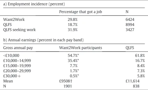
Table 1compares employment and earnings outcomes for the W2W participants and QLFS respondents. The raw data show that 30% of W2W participants found a job at some point in the period between them joining the scheme and the end of 2007,13_{compared to only 19%} for the out-of-work QLFS respondents in the period that they were ob-served in that survey. However, the full sample of non-employed QLFS respondents may not be an appropriate control group. Because of the voluntary nature of W2W, participants in that scheme have already by de_finition indicated their interest and motivation in_finding work. By contrast, some of the non-employed QLFS respondents may be unable or unwilling to work. The difference in the employment probabilities might then be explained by this difference in the motivation to_find work. Fortunately, the QLFS contains questions asking those of working age who are not currently working whether they want to work and whether they are looking for work. When the QLFS control group is re-stricted to individuals actually wanting and looking for work, then the proportion obtaining a job within the observed period rises to 32%, as shown in the third row ofTable 1a. Thus, without conditioning on individual characteristics, W2W participants are slightlylesslikely to have found work than job-seekers in the QLFS.

The raw data for earnings are shown inTable 1b. It is clear that those individuals who do obtain a job through W2W are likely to move into low-paid work, with 90% of those who found work accepting jobs for which they were paid less than £15,000 per year. This compares to 78% of the QLFS respondents in the control group. At the top end, signif-icantly more QLFS respondents who found a job received in excess of £30,000 per year, compared to W2W participants, and it is such individ-uals who cause the higher mean wage amongst QLFS relative to W2W workers.14_{On the other hand, the median wage is higher amongst the} W2W group, with the very lowest wage category covering a smaller proportion of such workers compared to the QLFS control group.

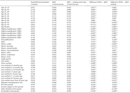
Such raw differences in outcomes, however, ignore systematic dif-ferences in characteristics between the two groups.Table A1in the Ap-pendix compares the background characteristics of the treatment and control groups, with a separate column for the job-seekers only, in the latter group. Looking at the differences between treatment and control groups, as reported in theﬁnal two columns, the data reveal that the W2W sample are on average younger, less well-educated, more likely to be a single parent, and less likely to be from an ethnic minority, rela-tive to the full QLFS sample. They are more likely to have recently worked, and less likely to have never worked at all. On average, W2W participants live in areas with higher unemployment rates.

There is little difference between groups in the likelihood of having no illness, which is perhaps surprising given the focus of W2W on IB claim-ants, though in terms of type of illness, the majority of those with illness in the W2W sample have mental health problems, whereas the QLFS has a much higher proportion with cardio illnesses.Banks et al. (2015)

have recently documented the growing proportion of disability beneﬁt claimants with mental health problems; and a recent OECD report has ex-plored the challenges in achieving higher labour market participation for

11

This is in contrast to an economy wide approach, such as that taken byVan Sonsbeek and Gradus (2006)andVan Sonsbeek and Alblas (2012)in their microsimulation analysis of a regime change in the Dutch disability scheme.

12

Very short duration jobs will not be observed in the QLFS group. If such jobs have low-er wages, we might expect to see lowlow-er avlow-erage wages for W2W participants, for whom short duration jobs are not ruled out.

13 _{This time frame means the early W2W participants have longer to}_ﬁ_{nd a job than QLFS} respondents, who are observed for a maximum of 15 months. This fact will be considered further in the following section.

14

(5)

this group (OECD, 2014). As expected, W2W participants are much more likely to be IB claimants than the QLFS control group.

When the W2W participants are compared to job-seekers only in the QLFS control group, some of these differences between the treated and the control group are much reduced, particularly in the case of age and duration out of work. Overall, the job-seekers in the QLFS ap-pear to be a more appropriate match for the W2W participants, and so from this point onwards, the control group will be limited to those wanting to work and looking for work.15_{Nevertheless, the}_ﬁ_{nal column} ofTable A1reveals that many signiﬁcant differences between W2W participants and job-seeking QLFS respondents remain, therefore requiring matching techniques to increase further the similarity of treatment and control groups.

4.2. Propensity score matching estimates of the impact of W2W

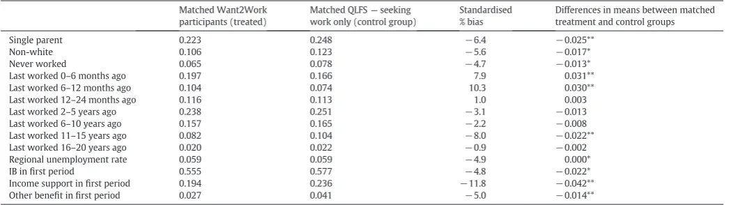
Before considering the evaluation results, it is important to check the balancing property of the PSM procedure.Table A1revealed some signif-icant differences in characteristics between the raw unmatched treatment and control groups. The matched sample will be balanced if there are no significant differences in the means of any of the characteristics between the treatment and control groups. Because of the concerns that the sam-ple of W2W participants may potentially differ compared to the typical unemployed individual, even when the latter group is restricted to job seekers, we experimented tofind the most balanced matched sample possible, while still retaining sufficient matched observations. This result-ed in a strict calliper of 0.00025 being chosen, and in the one-to-one matching, common support was not found for 2415 of the 6424 treated individuals, who were therefore dropped from the analysis.

Despite efforts to determine the most balanced sample possible, there remain some statistically signiﬁcant differences in the characteristics of the W2W participants and the QLFS respondents in the control group after the matching process.16_{In particular the W2W group has higher} proportions in the 16–19 year old (9.0% versus 6.9%) and 45–49 year old (10.6% versus 8.7%) age groups and a lower proportion in the 50– 54 year old age group (8.2% versus 10.5%), a higher proportion who are male (47.3% versus 42.8%) and lower proportions who are from an ethnic minority (10.6% versus 12.3%) and who are single parents (22.3% versus

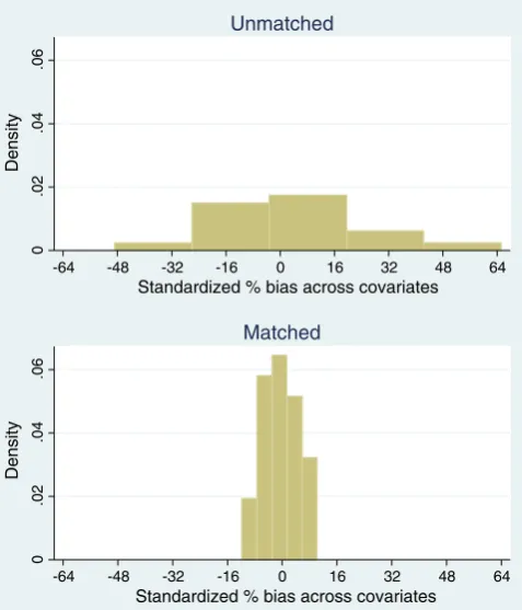
24.8%), a higher proportion with musculoskeletal (20.5% versus 18.6%) and a lower proportion with respiratory (2.2% versus 3.1%) health problems.17_{Furthermore, the W2W participants are more likely to have} shorter current unemployment spells and are less likely to be in receipt of benefits. Most of these differences favour the W2W group in terms of the probability of_finding work. However, these differences in observable characteristics in the matched sample are small. Only 2 differences, out of the 36 variables, have a standardised % bias of over 10%, and most are below 5%.18Fig. 1shows the % bias for each explanatory variable both in the raw (unmatched) and matched samples, whileFig. 2shows the histo-gram of the biases across all variables, again for the two samples.19_{It is} clear that the matching procedure has produced a substantially more bal-anced comparison between treatment and control groups, compared to the raw (unmatched) sample. The mean (median) standardized bias be-fore matching was 16.4% (10.8%), while after matching it is just 4.1% (3.4%). In a probit regression of the treatment indicator variable against all of the explanatory variables, if the treatment and control groups are similar in terms of their observable characteristics, then this regression should have no explanatory power. The pseudo R2_{in this regression} was 0.30 on the raw data sample, but just 0.02 on the matched data sam-ple, while the LR statistic for the joint insignificance of all of the explana-tory variables fell from 3427 to 238 when the matched sample was used. Although the treatment and control groups are not perfectly balanced, these results suggest a strong similarity in the observable characteristics of the treatment and control groups, and we therefore proceed to evaluate the W2W programme with this matched dataset.

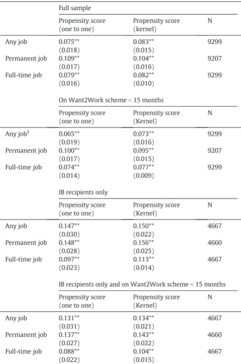
Table 2contains the core results of the evaluation, presenting the im-pact of W2W participation on the probability of moving into work, esti-mated using the PSM procedure described above. In each case, the results from the two types of matching procedures are presented, namely one-to-one (nearest neighbour) and kernel matching.

The_first panel inTable 2considers the full W2W and job-seeking QLFS samples. Thefirst row of results concerns movement into any employ-ment at any point, regardless of type of job and duration. The results show that those who participated in W2W are 8 percentage points more likely to move into employment than similar job-seekers from the QLFS control group. Recalling that the control group is restricted to QLFS respondents who did not live in a W2W pilot area, this means that indi-viduals in the W2W pilot areas who were looking to move back into em-ployment and participated in the W2W programme were 8 percentage points more likely tofind work than observationally similar individuals who were also looking for employment but did not live in W2W pilot re-gions and so could not participate. The W2W effect can therefore be seen as being over and above the effect of all other methods available nationally to help the unemployed back into work. This effect is both statistically and economically significant. Given that the average likelihood of moving into work in the sample is only around 30%, this impact of the W2W scheme is considerable. It is also very similar in size to the estimated effects of other active labour market policies such as Pathways to Work and the NDYP.

One possibility to explain their higher rate of moving into work is that W2W participants might be accepting jobs of lower quality. Two in-dicators of job quality that are available, other than wages which are considered later, are whether or not the job acquired is full-time,20 and whether or not the job acquired is permanent, or temporary and

15

In some respects, the QLFS job-seekers are actually less like the W2W participants than the full QLFS sample. This is particularly noticeable for education, with the lack of qualiﬁcations amongst the W2W participants even more noticeable when compared to only job-seekers.

16

The mean values for all explanatory variables within the matched dataset, with tests of signiﬁcance of the differences between treatment and control groups, are presented in

Table A2in the Appendix.

17

It is worth noting that while health problems are self-reported, reporting bias in spe-ciﬁc health problems is likely to be less than that for overall self-reported health (Jones et al, 2010).

18

The standardised % bias is the difference in the sample means as a percentage of the square root of the average of the sample variances in the treated and non-treated groups (Rosenbaum and Rubin, 1985).

19

Figs. 1 and 2were created using the graph andhistoptions on thepstestcommand, part of thepsmatch2command in Stata.

[image:5.595.43.293.77.228.2]

20_{A full-time job is de}_ﬁ_{ned as 30 hours or more per week. Of course, part-time work} need not be a signal of lower quality. A part-time job may have been actively desired by some individuals, particularly amongst those just getting over long-term health or disabil-ity problems, who compromise a large proportion of the W2W participants.

Table 1

Labour market outcomes for the treatment and control group.

a) Employment incidence (percent)

Percentage that got a job N

Want2Work 29.8% 6424

QLFS 18.7% 8994

QLFS seeking work 31.9% 3427

b) Annual earnings (percent in each pay band)

Gross annual pay Want2Work participants QLFS

b£10,000 54.7%* 61.8%

£10,000–14,999 35.4%* 16.7%

£15,000–19,999 7.7% 8.4%

£20,000–29,999 1.7%* 7.3%

£30,000 + 0.5%* 5.8%

Mean £9508† £11,614

N 1901 838

(6)

time-limited in some way.Gannon and Roberts (2011)for exampleﬁnd that older workers with health problems in Britain are less likely to work full-time. The second and third rows in each panel ofTable 2 con-sider these two possibilities in turn. The results show a larger W2W ef-fect on the probability of obtaining a permanent job than obtaining any job, with W2W participants being 10–11 percentage points more likely to acquire a permanent job than QLFS job-seekers. There is therefore no evidence that W2W is placing participants into casual jobs, in order to increase re-employment rates. When the analysis focuses on full-time jobs only, the results are very similar to those for‘any jobs’, with W2W participants being 8 percentage points more likely to move into full-time work than job-seekers in the QLFS.21

A potential caveat with the results presented so far is that W2W par-ticipants are potentially observed for longer than QLFS respondents, and that this might explain their apparent higher likelihood offinding work. Individuals respond to the QLFS forfive successive quarters, meaning that respondents in the QLFS control group are observed for a maximum of 15 months. W2W participants, however, are observed joining the scheme any time between the beginning of 2005 and the end of 2007, and so could be observed for considerably longer than 15 months, thus giving them more time to be observedfinding a job, relative to the QLFS out-of-work respondents. Thus, a new dependent variable was created to take the value of 1 if the W2W participant obtained a job within a max-imum of 15 months of joining the scheme. Anyone who obtained a job through W2W, but took longer than 15 months to do so was regarded as being unsuccessful, on the basis of this new variable. In actual fact, this meant that the analysis was now loaded against the W2W partici-pants, who if they joined the scheme in 2007 (45% of the W2W sample) were observed for fewer than 12 months, whereas the individuals in the QLFS control group are observed for a minimum of 12 months.22

The second panel inTable 2shows the results of this analysis. The impact of W2W on the employment probability is very similar to that estimated in theﬁrst panel, showing an estimated effect of 7 percentage points (compared to 8 percentage points in the uncensored sample).23

This estimate is the most conservative estimate produced in the paper, taking account of as many differences between treatment and control groups as possible, and so is our preferred result.

Similarly, the estimated W2W effects forfinding a permanent or full-time job when given a maximum of 15 months to do so, are very similar to the uncensored results in thefirst panel, with falls of only around one percentage point in the probability offinding a permanent job, and one-half a percentage point in the probability offinding a full-time job.

The analyses in the third and fourth panels ofTable 2repeat the anal-yses of thefirst two panels, but restrict the sample to those on IB only; these were the original target group of the W2W scheme, and an impor-tant aspect of the scheme is the availability of health care professionals to provide advice and support to help IB-recipients overcome their diffi cul-ties andfind suitable work. It might be expected, therefore, that if W2W is successful in helping people into employment, it will be most successful for this group. The results in the lower 2 panels confirm that this is indeed the case, with all estimated marginal effects being substantially larger than their equivalents in the upper two panels. Thus, thefirst row in the third panel shows that W2W participants who are in receipt of IB are 15 percentage points more likely to move into employment than job-seeking IB-recipients with similar characteristics in the control group. When only movements into jobs within 15 months of registering for W2W are considered, for compatibility reasons with the QLFS, W2W par-ticipants originally in receipt of IB are still 13 percentage points more like-ly tofind a job than their equivalents in the QLFS (panel 4, row 1). The impact of W2W onfinding permanent and full-time jobs is similarly larg-er for IB recipients only than for the full out-of-work population.

Table 3considers whether W2W participants whoﬁnd work earn more or less than their control group participants, adopting the same two methods of matching as used above. Since the wage data are banded, the midpoints of the bands are used, and then logged.24_{Estimates are}

24

For the open-ended top category (£30,000+), the value assigned to individuals is 1.5∗lower bound, i.e., £45,000. So few participants achieve a wage in this band, that the results are not signiﬁcantly affected if this value is changed.

0

.02

.04

.06

-64 -48 -32 -16 0 16 32 48 64

Standardized % bias across covariates

Density

Unmatched

0

.02

.04

.06

-64 -48 -32 -16 0 16 32 48 64

Matched

[image:6.595.40.279.56.228.2]

Density

Fig. 2.Histogram showing distribution of standardised % bias before and after matching.

-40 -20 0 20 40 60

Unmatched Matched

Fig. 1.Dot chart showing standardised % bias for each covariate before and after matching.

21

We further attempted to examine the permanence of W2W jobs via a postal survey, in February 2008, of all 804 participants who had found work by the end of 2006. The re-sponse rate was only 16% (131/804). Of these respondents, 72% reported that they had worked in the previous week, and of these, 73% were in the same job that they found through W2W. The representativeness of these respondents might be questioned, but the results suggest a good degree of permanence in the jobs found. Further details can be found inLindley et al. (2010).

22

We experimented with including a‘time entered programme’variable. Almost half of W2W respondents joined in the last year (2007); when we control for the fact that they did not have long toﬁnd a job, the estimated‘W2W’effects are increased. If anything, the estimates presented below are therefore under-estimates.

23

[image:6.595.308.547.58.337.2]

(7)

provided for the full sample, and for IB claimants only. All of the four esti-mated coefficients are negative but none approach statistical significance, and this has two probable causes. First, sample sizes are small, with only 1884 W2W participantsfinding work and having non-missing wage data. Second, and in particular, there are onlyfive wage bands in the data, and as shown inTable 1b, over half of those whofind work are in thefirst band, so there is little variation in earnings to explain.

Recall from above that both full-time and part-time workers are included in the analysis of wages. W2W respondents are more likely toﬁnd a full-time job than QLFS respondents,25and so are likely to have higher weekly wages for this reason. When the analysis is restrict-ed to full-time workers, the size of the negative coefﬁcients inTable 3

are increased, but they remain statistically insigniﬁcant.

4.3. Robustness checks of PSM results

In this section, we estimate further specifications, to check the robust-ness of the results to various modi_fications. The preferred speci_fication from the previous section (where the W2W treatment group is restricted tofinding work within 15 months, to maintain comparability with the

QLFS control group, and the outcome variable isﬁnding any job) is used as an example. If the various robustness checks described below are car-ried out on other estimates fromTable 2, the same robustness of results is observed, but they are not reported here for reasons of space.

First, the one-to-one matching results were checked for robustness to variation in the calliper used. As described in the previous section, a very strict calliper was used, as this produced the best result in terms of the balancing property of the matched treatment and control groups. As was seen, this resulted in a large number of observations being dropped due to falling outside the area of common support.Table 4

shows that as the calliper is gradually relaxed, fewer observations are lost for being off the common support. However, the estimated treatment effect of W2W is largely unaffected, remaining positive and significant. It actually increases from the base result of a 6.5 percentage point effect (fromTable 2and repeated in thefirst row ofTable 4) to an 8 percentage point effect with the wider calliper, though the change in the treatment effect is not significant.

The next check involved a variation in the matching process to try to ensure better matches, whereby individuals in the treatment and control group werefirst matched exactly according to one key characteristic, and then propensity score matching was used to match individuals across other characteristics within each category of thefirst variable. The overall treatment effect was then a weighted average of the treatment effects across all categories of thefirst variable. The key characteristics chosen to be exactly matched were age group, qualification level and type of ill-ness/disability. The analysis had to be undertaken by exactly matching on each of these variables in turn, cell sizes being too small to consider every combination of the three variables. The resulting overall treatment effects, again for the preferred specification of any job within a maximum period of 15 months, were 9.9 percentage points when matching exactly on age group,26_{4.6 percentage points when matching on highest quali}_fi -cation and 6.0 percentage points when matching on type of illness/ disability. The effects therefore remain positive and strong.

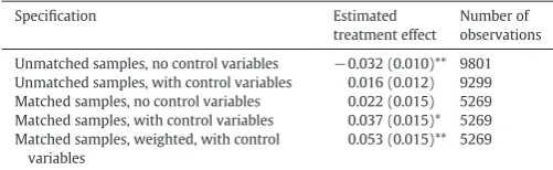
Table A2and the discussion in the previous section made it clear that although the matching process greatly reduces the differences between the treatment and control groups, some differences remain even after matching. To allow for this less than perfect matching, a further amend-ment is to take the matched samples of treated and control individuals, and rather than simply compare the mean values of the outcome variables in the two groups, estimate a regression on the matched samples, thus controlling for any remaining differences in observable characteristics between matched treatment and control groups. The results are shown inTable 5.

Theﬁrst two rows ofTable 5provide, for comparison purposes, estimated regression results on the unmatched samples. Since the de-pendent variable is a dummy variable, whether or not the individual ﬁnds a job within 15 months, the estimated equation is a probit, with

Table 5reporting the marginal effects on the W2W treatment variable. For the unmatched sample with no control variables, this marginal effect is negative and statistically signiﬁcant. This is analogous to the raw data inTable 1showing that the W2W sample is less likely toﬁnd work than

25

Of the W2W respondents who found a job, 58% were working full-time, compared to 42% for the QLFS.

[image:7.595.310.560.77.129.2]

26_{An interesting}_fi_{nding when matching on age group and then performing PSM within} each age group is that the estimated treatment effect is actually negative in the youngest two age groups, before turning positive and becoming larger with age for the remaining age groups. The W2W programme therefore seems to benefit older workers in particular, who perhapsfind it harder to return to employment without assistance.

Table 2

Propensity score estimates of W2W participation effect on probability of moving into work.

Full sample

Propensity score (one to one)

Propensity score (kernel)

N

Any job 0.075** 0.083** 9299

(0.018) (0.015)

Permanent job 0.109** 0.104** 9207

(0.017) (0.016)

Full-time job 0.079** 0.082** 9299

(0.016) (0.010)

On Want2Work schemeb15 months

Propensity score (Kernel)

N

Any job† 0.065** 0.073** 9299

(0.019) (0.016)

Permanent job 0.100** 0.095** 9207

(0.017) (0.015)

Full-time job 0.074** 0.077** 9299

(0.014) (0.009)

IB recipients only

N

Any job 0.147** 0.150** 4667

(0.030) (0.022)

Permanent job 0.148** 0.156** 4660

(0.028) (0.025)

Full-time job 0.097** 0.113** 4667

(0.023) (0.014)

IB recipients only and on Want2Work schemeb15 months

N

Any job 0.131** 0.134** 4667

(0.031) (0.021)

Permanent job 0.137** 0.143** 4660

(0.027) (0.022)

Full-time job 0.088** 0.104** 4667

(0.022) (0.015)

Notes:†denotes our preferred result. ** statistically signiﬁcant at the 1% level. * statistically signiﬁcant at the 5% level.

[image:7.595.43.291.84.458.2]

Matching variables are those listed inTableA2.

Table 3

Propensity score estimates of W2W participation effect on earnings.

Propensity score (one2one) Propensity score (Kernel) N

Full sample −0.026 −0.003 2578

(0.051) (0.037)

IB only −0.043 −0.033 1134

(0.144) (0.085)

(8)

the seeking-work control group from the QLFS. Once explanatory vari-ables are added to control for differences in characteristics between the two groups, then the estimated treatment effect turns positive but is sta-tistically insignificant. Row 3 shows a further increase in the estimated treatment effect when using the matched sample, thus no longer includ-ing those treated individuals whose characteristics mean that they_find no match in the control group. The fact that the treatment effect in-creases, relative to the unmatched sample results, shows that the treated individuals lying outside the area of common support are those whose characteristics make it particularly difficult for them tofind work. Once control variables are added to the probit equation on the matched sam-ple (row 4), to control for any remaining differences between treatment and control groups after matching, the effect of W2W is once again esti-mated to be positive and significant, at a 3.7 percentage point increase in the probability offinding work within 15 months.

Thefinal row inTable 5shows the estimated treatment effect when the probit equation estimated on the matched sample is further refined by using weights, with the weights provided by the kernel PSM showing the average closeness of each control observation to the treated obser-vations, and are thus an indicator of the quality of the observation in the matching process. It can be seen that in this specification, our pre-ferred probit specification, the effect of W2W is to increase the probabil-ity of employment within 15 months by 5.3 percentage points. Thus, using probit regression analysis after matching to further control for re-maining differences between treatment and control groups reduces the impact of W2W from 6.5 percentage points (Table 2) to 5.3 percentage points (Table 5), but the effect remains positive and significant. The small reduction in the estimated effect is due to the fact that in the matched sample, the remaining differences in mean characteristics be-tween treatment and control groups slightly favoured the treatment group in terms offinding work (see discussion ofTable A2above), and so controlling for these differences in the probit equation reduces the estimated treatment effect by a small amount.

Finally in this section, the analysis of earnings for those whoﬁnd work can be similarly extended, by estimating a regression equation on the matched sample identiﬁed by the PSM analysis. As with the em-ployment equations, this allows for any remaining differences between the treatment and control groups after matching to be controlled for. Using a regression-based estimator also allows us to take account of

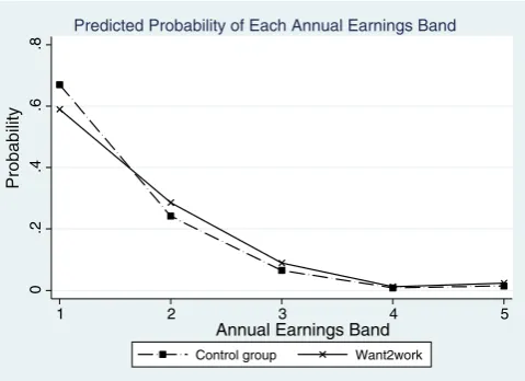
the grouped nature of the earnings variable, by estimating an interval regression model (seeStewart, 1983). This model is a Maximum Likeli-hood method, taking account of the earnings interval in which each ob-servation falls, and the upper and lower earnings limits of that interval, to produce a point estimate for each coefficient to indicate the condi-tional difference in earnings. The W2W coef_ficient in this second stage regression is−0.027 (standard error 0.050). An alternative to the inter-val regression is an ordered probit regression, taking account of just the earnings interval into which each observation falls, again estimated on the matched sample with weights obtained from the PSM.Fig. 3graphs the predicted probability of an individual, with mean characteristics, falling into each earnings interval, separately for the treatment and con-trol group. The difference between the two predicted probabilities is therefore the marginal effect of the W2W treatment on the probability of falling within each earnings interval. As can be seen, all of these mar-ginal effects are small, and all are statistically insigni_ficant.27_{All analyses} on the earnings data therefore tell the same story, that there is no significant difference in earnings between the W2W participants and the control group respondents who_find a job.

4.4. Differences in re-employment rates prior to the introduction of W2W

Most of the previous studies summarised in the literature review have adopted a DiD framework to evaluate active labour market policies. This approach was not adopted here, since the detailed database on W2W par-ticipants does not contain information covering the period before they joined W2W, and so could not be used in a DiD framework. However, as a robustness check on the results, and to mirror the methodologies used in other papers, we also conducted a comparison of employment out-comes in the W2W pilot and non-pilot areas, both before and after W2W was introduced, using QLFS in a DiD approach. Lookingﬁrst at the period before W2W was introduced, a comparison of re-employment probabilities between the areas that would become W2W pilot areas and those that would not, reveals whether those individuals who lived in W2W areas always had a higher re-employment rate, perhaps because of a particular feature of the local labour market for example.

QLFS data with a local area indicator at a sufﬁciently disaggregated level are available from 2003. Since the W2W pilot programme began in September 2004, we use data up to the second quarter of 2004 (i.e., up to June 2004). If we wanted to follow individuals for allﬁve quarters in which they participate in the QLFS, then this meant only two cohorts of respondents could be followed. This produced too few out of work job-seekers in the W2W areas for feasible analysis, however. Therefore we restrict the analysis to three quarters of QLFS data, considering indi-viduals out of work but seeking work in one quarter, and looking to see whether they move into work in the subsequent two quarters. This allowed us to follow six cohorts of respondents.

The local area indicator is used to determine whether or not individ-uals live in an area that will become a W2W pilot area.28_{The same} anal-ysis as used in the previous section is repeated, estimating the difference in the likelihood of job-seekers moving into work when comparing (future) W2W and non-W2W areas. PSM is again used, matching on ex-actly the same list of characteristics. The results show a higher rate of moving into a job in the areas that will become W2W pilot areas, though the difference is highly statistically insigniﬁcant. The estimated effect (standard error) is 0.020 (0.101) when using one-to-one matching.29_A similar analysis was then undertaken for the W2W period, but again

27

The estimated marginal effects for the W2W treatment for theﬁve earnings intervals are (standard errors in parentheses): Interval 1−0.054 (0.053); Interval 2 0.027 (0.027); Interval 3 0.017 (0.016); Interval 4 0.003 (0.003); Interval 5 0.007 (0.007).

28 _{Only those individuals who remain in that area throughout the 3 quarters they were} observed were included.

29

[image:8.595.33.284.631.708.2]

Unfortunately it was not possible to do a similar pre-W2W exercise for IB claimants only. Every job-seeking IB claimant in the QLFS in W2W areas before W2W began failed to move into a job within three quarters.

Table 5

Probit equations forﬁnding a job within 15 months, various speciﬁcations.

Speciﬁcation Estimated

treatment effect

Number of observations

Unmatched samples, no control variables −0.032 (0.010)** 9801 Unmatched samples, with control variables 0.016 (0.012) 9299 Matched samples, no control variables 0.022 (0.015) 5269 Matched samples, with control variables 0.037 (0.015)* 5269 Matched samples, weighted, with control

variables

0.053 (0.015)** 5269

Notes: reported treatment effect is the estimated marginal effect derived from the probit coefficients. ** statistically significant at the 1% level. * statistically significant at the 5% level.

Control variables are those listed inTableA2. Table 4

Impact of varying the calliper: one-to-one matching, outcome variable‘get any job’, Indi-viduals on Want2Work scheme restricted tob15 months (i.e., preferred speciﬁcation in

Table 2).

Calliper Number of observations off common support (%)

Number of observations used

Estimated treatment effect of Want2Work

0.00025 2415 (37.6%) 6884 0.065 (0.019)** 0.0005 999 (15.6%) 8300 0.074 (0.017)**

0.001 204 (3.2%) 9095 0.080 (0.018)**

0.005 1 (0.002%) 9298 0.080 (0.021)**

(9)

using QLFS data, rather than the W2W database used in the previous sec-tion. As with the pre-W2W period, the cohorts were again followed for three quarters, in order to make a fair comparison. The results therefore produce the‘intention to treat’estimator, based on individuals selected for potential treatment (by virtue of living in a Wamt2Work area) though not necessarily actually treated (in terms of participating in W2W). The results show a W2W effect on moving into employment of 0.049 (0.113). This is again insigniﬁcantly different from zero, and so also insig-niﬁcantly different from the pre-W2W effect. This however is due to the large standard errors in turn caused by small numbers of on support treat-ed observations (i.e., few people in the pilot areas in the QLFS who were initially out of work but looking for work). In terms of the point estimate, it has increased 2.5 times from a 2 percentage point effect to a 4.9 percent-age point effect which is at least supportive of the positive effect observed for W2W in the main analysis above.30_{The DiD estimate is therefore 2.9} percentage points, calculated as:

d

DiD¼ ET1−E

C

1

− ET0−E

C

0

whereEis the estimated re-employment rate, theTandCsuperscripts de-note treatment and control groups and the 0 and 1 subscripts dede-note pre-and post-W2W periods, respectively.

5. Summary and conclusion

The W2W pilot scheme was aimed at helping beneﬁt recipients, pri-marily those receiving IB, back into employment, using a range of advice and incentive mechanisms. By using PSM to compare W2W participants with similar job-seekers in non-W2W regions we were able to evaluate the success of the W2W programme.

The evidence produced is convincing, and supportive of W2W. Using a range of estimation methods, different sub-samples, and dif-ferent types of job, the W2W participants consistently come out as being more likely to move into employment, compared to individ-uals in the control group. Such an advantage was not observed in the W2W areas before the programme was introduced. The size of the programme effect varies according to the speciﬁcation being considered, but is always statistically signiﬁcant. Our preferred

specification is the most conservative one; allowing W2W partici-pants a maximum of 15 months tofind a job (as this is the longest that we can observe individuals in the control group), and comparing them to out-of-work QLFS respondents who say that they actually want a job and are looking for a job, but do not live in the W2W pilot areas and so could not participate in the programme. The re-sults show that the W2W participants are 7 percentage points more likely to move into employment than those observationally-similar individuals looking for work in non-pilot areas, showing the benefit of W2W over and above the standard help on offer to the un-employed. Given that only around 30 percent of jobseekers across the two datasets obtained a job, this W2W effect is sizeable. The size of this effect is very similar to the estimated effects of other ac-tive labour market policies, such as the 5 percentage point effect on employment of the New Deal for Young People, as estimated by bothBlundell et al. (2004)andDe Giorgi (2005).

The original target of W2W was individuals in receipt of IB, and the programme was tailored to help that group in particular, for ex-ample through the involvement of health professionals. When the treatment and control groups are restricted to those individuals ini-tially in receipt of IB, the estimated employment impact of W2W in-creases to around 13 percentage points, against a base of 25 percent of IB claimants moving into employment within 15 months. The size of this effect compares very favourably with the Pathways to Work scheme, for which researchers have found employment effects of 7–9 percentage points using parametric methodology (Adam et al., 2006; Bewley et al., 2007).

As well as considering simply whether a job is obtained, the analysis also provided some evidence as to the quality of jobs being obtained. In terms of the type of job accepted, the results are not changed greatly when the focus is restricted to only full-time or permanent jobs, though the W2W effect is slightly weaker for obtaining full-time work than for obtaining any job in the case of former IB claimants. Even in this case, however, the W2W effect compared to the control group is strongly pos-itive. In terms of earnings, there is some evidence that W2W participants accept lower wage jobs than members of the control group, though this difference is not statistically signiﬁcant. Overall, there is nothing to sug-gest that the success of W2W in terms of getting people into work can be explained by a greater willingness to push clients into low quality jobs. Finally, on a methodological note, this paper shows how evalua-tions of labour market policies can be undertaken, even when policy-makers have not collected data on a control group of non-participants, or on participants before involvement, thus ruling out DiD techniques. Data from national surveys such as Labour Force Surveys can be used to obtain a sample of individuals in non-policy areas, who can then be matched to programme participants using PSM techniques, to ensure the employment probabilities of similar individuals are being compared. Such non-parametric techniques have additional advantages over more traditional evaluation tech-niques, in that they do not impose functional form, and identify any individual for whom there is a lack of common support. Howev-er, these techniques should be seen as a fall-back position, to be re-served for situations when a control group has not been established as part of the design. A properly controlled prospective evaluation is still to be preferred.

Acknowledgements

This work was produced for the National Assembly for Wales, con-tract number 130/2006. All views expressed are those of the authors, and not necessarily those of the National Assembly. The Labour Force Survey data used in the report were made available by the UK Data Ser-vice. The database of information on W2W participants was provided by the Welsh Assembly Government. We thank two anonymous referees and the editor for very useful comments.

30_{The W2W effect of 5 percentage points using the QLFS data is less than the W2W effect} of 8 percentage points using the W2W database. The main results using the database esti-mated an average treatment effect for individuals actually treated by the programme. The QLFS results, on the other hand, estimates only an‘intention to treat’effect, on individuals who were eligible for treatment (though not all will have actually been treated).

0

.2

.4

.6

.8

1 2 3 4 5

Annual Earnings Band

Control group Want2work

Predicted Probability of Each Annual Earnings Band

[image:9.595.48.288.54.228.2]

Probability

(10)

[image:10.595.35.552.107.479.2]

Table A1

Sample means for Want2Work participants and QLFS respondents (unmatched samples).

Want2Work participants (treated)

QLFS (control group)

QLFS—seeking work only (control group)

Difference W2W—QLFS Difference W2W—QLFS seeking

Age 16–19 0.077 0.050 0.079 0.027** −0.002

Age 20–24 0.149 0.066 0.086 0.083** 0.062**

Age 25–29 0.144 0.071 0.085 0.073** 0.059**

Age 30–34 0.123 0.096 0.105 0.028** 0.018**

Age 35–39 0.137 0.115 0.122 0.021** 0.014*

Age 40–44 0.130 0.109 0.123 0.021** 0.007

Age 45–49 0.102 0.100 0.103 0.002 −0.001

Age 50–54 0.073 0.112 0.107 −0.039** −0.034**

Age 55–59 0.052 0.165 0.113 −0.113** −0.061**

Age 60 plus 0.014 0.116 0.076 −0.102** −0.062**

Highest qualiﬁcation: NQF5 0.041 0.090 0.105 −0.049** −0.064**

Highest qualiﬁcation: NQF1 0.154 0.137 0.155 0.017** −0.001

No qualiﬁcations 0.498 0.336 0.269 0.162** 0.229**

Male 0.493 0.342 0.440 0.151** 0.053**

Illness: cardio 0.026 0.120 0.109 −0.095** −0.083**

Illness: learning 0.017 0.032 0.030 −0.015** −0.013**

Illness: mental health 0.249 0.081 0.072 0.167** 0.177**

Illness: musculoskeletal 0.193 0.204 0.186 −0.011 0.007

Illness: other 0.126 0.106 0.095 0.021** 0.031**

Illness: respiratory 0.019 0.052 0.057 −0.033** −0.038**

Illness: none 0.371 0.405 0.450 −0.034** −0.079**

Single parent 0.211 0.152 0.192 0.059** 0.019*

Non-white 0.099 0.117 0.111 −0.018** −0.012

Never worked 0.053 0.151 0.122 −0.098** −0.068**

Last worked 0–6 months ago 0.208 0.101 0.192 0.107** 0.016

Last worked 6–12 months ago 0.108 0.059 0.089 0.050** 0.019**

Last worked 12–24 months ago 0.118 0.085 0.114 0.033** 0.004

Last worked 2–5 years ago 0.257 0.169 0.162 0.088** 0.095**

Last worked 6–10 years ago 0.148 0.194 0.164 −0.046** −0.016*

Last worked 11–15 years ago 0.072 0.110 0.088 −0.038** −0.016**

Last worked 16–20 years ago 0.018 0.056 0.036 −0.038** −0.018**

Last worked more than 20 years ago 0.018 0.075 0.033 −0.058** −0.015**

Regional unemployment rate 0.059 0.049 0.050 0.010** 0.010**

IB inﬁrst period 0.597 0.335 0.256 0.262** 0.342**

Income support inﬁrst period 0.191 0.091 0.107 0.100** 0.084**

Other beneﬁt inﬁrst period 0.022 0.075 0.160 −0.053** −0.139**

No beneﬁt inﬁrst period 0.190 0.516 0.495 −0.326** −0.305**

Note: QLFS is the GB Quarterly Labour Force Survey.

Table A2

Mean values of explanatory variables within the matched treatment and control groups.

Matched Want2Work participants (treated)

Matched QLFS—seeking work only (control group)

Standardised % bias

Differences in means between matched treatment and control groups

Age 16–19 0.091 0.069 8.1 0.022**

Age 20–24 0.132 0.125 2.3 0.007

Age 25–29 0.127 0.124 1.0 0.003

Age 30–34 0.117 0.111 2.0 0.006

Age 35–39 0.137 0.137 0.0 0.000

Age 40–44 0.129 0.134 −1.4 −0.005

Age 45–49 0.106 0.087 6.0 0.019**

Age 50–54 0.082 0.105 −7.6 −0.023**

Age 55–59 0.063 0.073 −3.5 −0.010

Highest qualiﬁcation: NQF5 0.045 0.039 2.4 0.006

Male 0.473 0.428 9.1 0.045**

Illness: cardio 0.032 0.038 −2.4 −0.006

Illness: learning 0.019 0.016 1.5 0.003

Illness: mental health 0.201 0.191 2.8 0.010

Illness: musculoskeletal 0.205 0.186 4.7 0.019*

Illness: other 0.121 0.118 0.9 0.003

Illness: respiratory 0.022 0.031 −4.4 −0.009*

[image:10.595.37.553.537.745.2]

(11)

References

Adam, S., Emmerson, C., Frayne, C., Goodman, A., 2006.Early quantitative evidence on the impact of the pathways to work pilot. Research Report No. 354, Department for Work and Pensions.

Banks, J., Blundell, R., Emmerson, C., 2015.Disability beneﬁt receipt and reform: reconcil-ing trends in the United Kreconcil-ingdom. J. Econ. Perspect. 29 (2), 173–190.

Bewley, H., Dorsett, R., Haile, G., 2007.The impact of Pathways to Work. Research Report No. 435, Department for Work and Pensions.

Bewley, H., Dorsett, R., Ratto, M., 2008.Evidence on the effect of pathways to work on existing claimants. Research Report No. 488, Department for Work and Pensions.

Blundell, R., Costa Dias, M., Meghir, C., Van Reenen, J., 2004.Evaluating the employment impact of a mandatory job search program. J. Eur. Econ. Assoc. 2, 569–606.

Brown, S., Taylor, K., 2011.Reservation wages, market wages and unemployment: analy-sis of individual level panel data. Econ. Model. 28, 1317–1327.

Caliendo, M., Kopeinig, S., 2008.Some practical guidance for the implementation of pro-pensity score matching. J. Econ. Surv. 22, 31–72.

De Giorgi, G., 2005.The New Deal for Young Peopleﬁve years on. Fisc. Stud. 26, 371–383.

Dorsett, R., 2001.The New Deal for Young People: relative effectiveness of the options in reducing male unemployment. Discussion Paper No. 7, PSI.

Gannon, B., Robert, J., 2011.Part-time work and health among older workers in Ireland and Britain. Appl. Econ. 43, 4749–4757.

Jones, A.M., Rice, N., Roberts, J., 2010.Sick of work or too sick to work? Evidence on self-reported health shocks and early retirement from the BHPS. Ecol. Model. 27, 866–880.

Leuven, E., Sianesi, B., 2003. PSMATCH2: Stata Module to Perform Full Mahalanobis and Propensity Score Matching, Common Support Graphing, and Covariate Imbalance Testing.http://ideas.repec.org/c/boc/bocode/s432001.html(This version, Version 4.0.5 18 April 2012).

Lindley, J., Mcintosh, S., Roberts, J., Czoski Murray, C., Edlin, R., 2010.Usingﬁnancial incen-tives and improving information to increase labour market success: a non-parametric evaluation of the‘Want2work’programme. Discussion Paper No. 2010013, Shefﬁeld Economics Research Paper Series.

Martin, P., 2015.Activation and active labour market policies in OECD countries: stylised facts and evidence on their effectiveness IZA journal of labor. Policy 4.

Mcvicar, D., Podivinsky, J., 2009.How well has the New Deal for Young People worked in the UK regions? Scott. J. Polit. Econ. 56, 167–195.

Oecd, 2014.Mental health and work: United Kingdom Paris and Washington. Organisa-tion for Economic Co-operaOrganisa-tion and Development, D.C.

Rosenbaum, P., Rubin, D., 1983.The central role of the propensity score in observational studies for causal effects. Biometrika 70, 41–55.

Rosenbaum, P., Rubin, D., 1985.Constructing a control group using multivariate matched sampling methods that incorporate the propensity score. Am. Stat. 39, 33–38.

Stewart, M.B., 1983.On least squares estimation when the dependent variable is grouped. Rev. Econ. Stud. 50, 737–753.

Van Sonsbeek, J.-M., Alblas, R., 2012.Disability beneﬁt microsimulation models in the Netherlands. Econ. Model. 29, 700–715.

[image:11.595.42.567.68.215.2]

Van Sonsbeek, J.M., Gradus, R.H.J.M., 2006.A microsimulation analysis of the 2006 regime change in the Dutch disability scheme. Econ. Model. 23, 427–456.

Table A2(continued)

Matched Want2Work participants (treated)

Matched QLFS—seeking work only (control group)

Standardised % bias

Differences in means between matched treatment and control groups

Single parent 0.223 0.248 −6.4 −0.025**

Non-white 0.106 0.123 −5.6 −0.017*

Never worked 0.065 0.078 −4.7 −0.013*

Last worked 0–6 months ago 0.197 0.166 7.9 0.031**

Last worked 6–12 months ago 0.104 0.074 10.3 0.030**

Last worked 12–24 months ago 0.116 0.113 1.0 0.003

Last worked 2–5 years ago 0.238 0.251 −3.1 −0.013