This is a repository copy of Why are aggregate equity payouts pro-cyclical?. White Rose Research Online URL for this paper:
http://eprints.whiterose.ac.uk/111969/ Version: Accepted Version
Article:
Huang-Meier, Winifred, Freeman, Mark C orcid.org/0000-0003-4521-2720 and Mazouz, Khelifa (2015) Why are aggregate equity payouts pro-cyclical? Journal of
Macroeconomics. pp. 98-108. ISSN 0164-0704 https://doi.org/10.1016/j.jmacro.2015.01.005
Reuse
This article is distributed under the terms of the Creative Commons Attribution-NonCommercial-NoDerivs (CC BY-NC-ND) licence. This licence only allows you to download this work and share it with others as long as you credit the authors, but you can’t change the article in any way or use it commercially. More
information and the full terms of the licence here: https://creativecommons.org/licenses/ Takedown
If you consider content in White Rose Research Online to be in breach of UK law, please notify us by
Why are aggregate equity payouts pro-cyclical?
Winifred Huang-Meiera,*, Mark C. Freemanb and Khelifa Mazouzc
a Aston Business School, Aston University, Birmingham, B4 7ET, United Kingdom
b School of Business and Economics, Loughborough University, Leicestershire,
LE11 3TU, United Kingdom
c Cardiff Business School, Cardiff University, Aberconway Building, Colum Drive
Cardiff, CF10 3EU, United Kingdom
* Corresponding author. Tel.: +44 121 204 3490; fax: +44 121 204 4915 E-mail addresses: [email protected] (W. Huang-Meier),
[email protected] (M.C. Freeman), [email protected] (K. Mazouz)
ABSTRACT
We use two general equilibrium models to explain why changes in the external
economic environment result in pro-cyclical aggregate dividend payout behavior.
Both models that we consider endogenize low elasticity of investment. The first
model incorporates capital adjustment costs, while the second one assumes that
shareholder wealth. We show that, while both models generate pro-cyclical
aggregate dividends, a feature consistent with the observed business-cycle pattern
of payouts from well-diversified portfolios, the second model provides a more
likely explanation for this effect. Our findings emphasize the importance of
incorporating agency conflicts when considering the relationship between the
external economic environment and the financial behavior of businesses.
Keywords: dynamic stochastic general equilibrium economies; payout policy;
business fluctuations; firm objectives; capital adjustment costs
JE: C63, C68, G35, E32, L21, E22
1 Introduction
The observed correlation coefficient between the real aggregate dividends paid by
firms and real GDP in the U.S. has been around +0.50 for many years.1 This
phenomenon suggests that the payout policies of businesses are systematically
and strongly affected by external changes in the economic environment. However,
this clearly observed aggregate dividend pro-cyclicality is inconsistent with the
predictions of large parts of the existing theoretical literature.2 Many general
equilibrium models imply that investors should benefit from holding a portfolio
with counter-cyclical equity payouts (e.g., Alessandrini, 2003; Carceles-Poveda,
2009; Jermann and Quadrini, 2012). These predictions arise because, in economic
booms, many potentially profitable investment opportunities are available to firms
who wish to reinvest. In addition, since the marginal utility of consumption is
low during strong economic conditions, investors are less likely to depend on
dividend income at this time.
In this paper, we describe two dynamic stochastic general equilibrium
(DSGE) models to explain why external changes in the economic environment
should result in pro-cyclical aggregate equity payout behavior. We model an
environment where firms and households simultaneously undertake constrained
optimizations and market clearing conditions ensure that the economy remains in
equilibrium. As a consequence, dividend and investment decisions are made
simultaneous and neither is a ‘residual’ of the other.
In the first set of models, managers aim to maximize their current share
price while firms experience capital adjustment costs. This follows an extensive
literature that is based on the observation that managers cannot immediately and
perfectly adjust their real investment decisions (see, e.g., Jermann, 1998; Boldrin
et al., 2001; Cooper and Haltiwanger, 2006; Gershun, 2010; Santoro and Wei,
2011). This investment friction has previously played an important role in
explaining a number of asset pricing phenomena based upon DSGE models. Both
Jermann (1998) and Danthine and Donaldson (2002) have exploited it to present
potential resolutions to the equity premium puzzle. Christiano and Fisher (1995),
by contrast, apply adjustment costs to Tobin’s Q and show that adjustments costs
are related to the cyclical properties of equity prices and investment goods.
In our second set of models we assume that there are no frictions, but
agency conflicts exist. Specifically, we assume that managers maximize their own
expected utility function rather than shareholders’ wealth (see, inter alia, Radner,
1970; Sandmo, 1971; Leland, 1972; Carceles-Poveda, 2005, 2009). This choice
exploits the known similarity between models that incorporate risk-averse
managers and those with capital adjustment costs. In particular, Carceles-Poveda
(2003) has shown that, with appropriately matched parameter values, the
equilibrium behavior of these two economies around the steady state is identical.
A common key feature among these models is that they endogenize low
elasticity of investment. When this feature is combined with investors’ desire for
dividend income as a source of consumption, more (less) money becomes
available to pay out to shareholders in economic booms (recessions). This
models endogenize low elasticity of investment, if one model predicts
pro-cyclical dividends then so should the other; we confirm that here. However, we
also show that the cyclicality of optimal dividend behavior is clearly distinct
between the two models and, as a consequence, each is not equally plausible as an
explanation. We find that while the required level of managerial risk aversion
falls at the lower end of standard ranges, relatively high levels of capital
adjustment costs are required to explain observed payout and consumption
behavior. This evidence suggests that the economy with risk-averse managers
offers a more realistic explanation to the dividend pro-cyclicality phenomenon.
This conclusion is supported by the observation that the agency conflict model
results are more robust to changes in the choice of parameter values.
In order to test the overall performance of our DSGE models, we consider
their explanatory power for a set of macroeconomic variables. This captures the
pro-cyclicality and volatility of four variables: dividends, consumption, labor
hours worked, and investment. The performances of the preferred specifications
across the entire range of these diagnostics are the best amongst all the models
considered. Resolving the anomaly of pro-cyclical aggregate dividends through
either agency conflicts or capital adjustment costs comes with the additional
benefit of increasing the overall ability of these models to explain the broader
This paper is most naturally compared with important recent studies by
Carceles-Poveda (2009) and Jermann and Quadrini (2012). Carceles-Poveda
(2009) focuses on the sensitivity of aggregate behavior to household
heterogeneity in an incomplete market economy both in the presence and absence
of utility maximizing managers. Jermann and Quadrini (2012), by contrast,
explain pro-cyclical equity payments through economy-wide financial shocks. We
present a number of new findings. First, we show that the pro-cyclicality of
dividends can be explained in simple agency-conflict models with representative
agents and no frictions. Second, we demonstrate that agency conflicts are more
likely to resolve the dividend cyclicality puzzle than capital adjustment costs.
Third, we extend the representative household’s utility function to allow for the
presence of internal multiplicative habit formation; a feature that generally makes
household consumption smoother (see, for example, Constantinides, 1990).
Finally, we present detailed sensitivity analysis that demonstrates that the
pro-cyclicality of dividends will emerge in the utility maximizing manager model for
a wide range of plausible parameter values.
The remainder of the paper is structured as follows. Section 2 presents the
economic environment of the utility-maximizing manager, the value-maximizing
firms with capital adjustment costs, and the “basic” model that has neither of
2 Economic Environment
This section presents two economic models that can potentially explain the
pro-cyclicality of aggregate payout policy. The first model is based on a
value-maximizing firm with capital adjustment costs (VM-CAC hereafter), while the
second one assumes that managers maximize their own objective function rather
than shareholders’ wealth (UM hereafter). We initially present the assumptions
that both models have in common and then introduce the differences.
2.1 The Firm and Household
The tax-free economy consists of a representative firm that is all-equity financed
with one share in issue and a representative agent. There are no other investment
opportunities available and, with the exception of capital adjustment costs in the
VM-CAC model, there are no frictions.3
At any given time, , the output, , from the representative firm is given
by a standard Cobb-Douglas production function that depends on both the capital,
, and normalized labor hours, , employed:
3 With the exception of all-equity financing, these assumptions are identical to Jermann and Quadrini (2012).
where and x denote a stochastic technology shock and the deterministic trend
in labor augmenting technical change respectively. The parameters and 1 −
are output elasticities of capital and labor, respectively.4 The d superscript on
denotes a firm’s demand for labor. The technology shock process is assumed to
follow a first order autoregressive process (AR(1)) in logs and evolves
exogenously as follows: ln ln , where is the parameter of
persistence and is an independent and identically normally distributed random
variable . The representative firm also pays dividends, , to equity
owners:
where is the wage rate and is the amount re-invested by the firm.5 By
controlling for the initial inputs and , other variables (equity payouts, output
and investment) are simultaneously endogenized along with the household’s
problem.
Many DSGE models are built with a time-separable utility function, which
assumes that the representative household’s preferences are independently
4See also Jermann (1998) for more details on the specification of the firm’s production function.
5 See, for example, Lang and Litzenberger (1989), Alli et al. (1993) and Baker and Smith (2006).
determined by consumption and leisure in each period. In addition, the
representative’s utility that is derived from current consumption is independent of
past consumption behavior. In line with Constantinides (1990) and others, we
extend the utility function to incorporate internal habit formation.6 In this case, the
representative household’s level of satisfaction from consumption is determined
not only by current consumption but also by past consumption.
Constantinides (1990) shows that this feature resolves Mehra and
Prescott’s (1985) equity premium puzzle and generally results in smoother
optimal household consumption patterns. In this case, the household’s objective
function is:
for is the consumption of the household, determines the
time devoted to market activities (Campbell, 1994 and Cooley and Prescott,
1995), denotes the hours worked, determines the strength of the habit motive
and is the coefficient of relative risk aversion (CRRA) of the household. The s
6 See, for example, Constantinides (1990), Carroll (2000), Carroll et al. (2000), Dynan (2000), Boldrin et al. (2001), Seckin (2001), Otrok et al. (2002), Gershun (2010) among others.
max
superscript on denotes the supply of labor. is the time discount factor. Labor
hours worked are normalized so that denotes the time available for leisure.
In this framework, consumption comes from two sources. First, the
household receives labor income of . Second, it can choose to hold
shares in the representative firm. Cash can then be generated from this equity
holding both from the dividend and by selling shares at the market
price . The household budget constraint determines this price of equity:
2.2 The Manager Objective Function and the Capital Accumulation
Process
Differences between the “basic” model, the UM model, and the VM-CAC model
arise from the managers’ objective function, , and the process that determines
the evolution of capital within the firm.
Managers have control over two variables ( and ) at any time, , to
maximize their objective function. In both the “basic” and VM-CAC models, the
assumption is that managers aim to maximize shareholder wealth, . By
contrast, following Radner (1970), Sandmo (1971) and Leland (1972), among
others, the UM model is based on the assumption that managers are risk-averse
and act in a way that satisfies their own personal objective function rather than
maximizing the share price of their firm. Carceles-Poveda (2005, 2009) shows
that the risk aversion assumption improves our understanding of managers’
behavior. We summarize the manager’s objective function as:
where is the coefficient of relative risk aversion of the manager and is the
subjective discount factor. This is an appropriate utility function if managers’
income comes solely from income derived from the ownership of equity in his/her
own firm.7 There is some support for this from studies, which show how poorly
diversified entrepreneur’s portfolios often are; e.g., Heaton and Lucas (2000).
Alternately, we might imagine that the manager is rewarded though a salary and
bonus policy that is linked to the firm’s dividend payouts. This managerial utility
function has previously been used by Carceles-Poveda (2003).
The second key difference between the “basic” model, the UM model, and
the VM-CAC model is related to the capital accumulation process. In the “basic”
and UM models, the capital employed in the firm develops according to
7While, under this assumption, the manager’s salary comes entirely from dividends, it is also necessary to assume that the manager holds an infinitesimally small fraction of the equity. This is because, within this model, all dividends go to the household. We thank an anonymous referee for this point.
max UM
max VM CAC
, where denotes the capital depreciation rate. By contrast,
in the VM-CAC model, the capital accumulation process is given by
where is a concave capital adjustment cost function and determines the
level of capital adjustment costs. Given this economic friction, the elasticity of
investment is expected to be lower than in a model without CAC. Specifically,
we follow Gershun (2010) and set
Notice that, the lower the value of , the higher the capital adjustment cost.
Ultimately, as , the capital adjustment cost goes to zero and the VM-CAC
model becomes the “basic” model. We refer to this last case as the “VM-no-CAC
model”.
2.3 Equilibrium Conditions
General equilibrium exists in this economy when both the firm and the household
are able to simultaneously maximize their objective functions. This leads to five
first-order conditions that can be algebraically rearranged to give:
(6)
where is the household’s inter-temporal marginal rate of
substitution of consumption between times and . Notice that the last of
these equations is just the standard Euler equation that is used widely in asset
pricing.
In addition to these conditions, labor and capital markets must clear. This
leads to three further constraints. First, the supply and demand of labor must be
equal, . Second, the firm has one share in issue at all times, .
Finally, output must be either consumed or re-invested, .
To simultaneously solve this set of six equations, we use Dynare software
in conjunction with Matlab. This allows us to determine the steady state growth
rates of several underlying macroeconomic and financial variables, together with
UM
VM CAC
(8)
(9)
a variance-covariance matrix of the growth rates of each of these variables, and
impulse response functions.8
2.4 Calibration
This subsection describes the parameter values used in our baseline calibrations.
Further evidence on the sensitivity of our results to the parameter values is
provided in subsection 3.1.
For the Cobb-Douglas production function, the values of the capital
elasticity of output , the depreciation rate , and the quarterly
trend in labor augmenting technical change x are taken from Kydland
and Prescott (1982) and Jermann (1998). These values are also commonly used in
long-term economic and finance models (e.g. Hansen, 1985; Campbell, 1994;
Jermann, 1998). In line with Hansen (1985), the stochastic technology shock ( )
follows an AR(1) process with a persistence parameter and standard
deviation .
For the household, we choose , which is standard in the literature
(e.g. Hansen, 1985; Prescott, 1986; Campbell, 1994; and Jermann, 1998). We
follow Carceles-Poveda (2003) by setting . The value of falls within
the 1 to 5 range, which is again generally considered reasonable by many
economists (e.g. Jermann, 1998; Carceles-Poveda, 2003; and Gershun, 2010). In
8
the sensitivity analysis, we vary between 0 and 100. The estimated value of the
agent’s internal consumption habit persistence parameter is equivalent
to the figure estimated by Jermann (1998). The value for the time
devoted to market activities is obtained from Campbell (1994).9
Following Carceles-Poveda (2003), we set manager’s stochastic subjective
discount factor to . We also set the manager’s risk aversion coefficient
to and 5 to indicate low and high levels of risk aversion, respectively.
Both these risk aversion values lie within the one to five range that many
economists consider to be realistic (e.g., Ljungqvist and Sargent, 2004; Parrino et
al., 2005; and An and Cheung, 2010). We also vary this figure between 0 and 100
to examine the sensitivity of dividend cyclicality to the manager’s degree of risk
aversion.
In the VM-CAC economy, the parameter value determining capital
adjustment costs is set to (1) for relatively low capital adjustment costs
9
following Gershun (2010) and (2) for relatively high capital adjustment
costs, which is similar to the value used by Jermann (1998).
3 Results
We report the results for six models, each both with ( and without (
household habit formation, giving a total of twelve models. The first is the
“basic” VM-no-CAC economic framework with no capital adjustment costs and a
manager who aims to maximize shareholder wealth; this is the standard DSGE
model. The next three models are for the utility maximizing (UM) manager with
different levels of risk aversion; risk neutrality and both low
and high risk aversion. The final two models are low ( )
and high ( ) capital adjustment cost VM-CAC models.
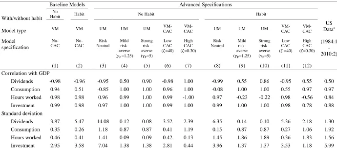
In Table 1 we report eight summary statistics for each model. These refer
to the cyclicality and volatility of dividends, consumption, labor hours, and
investment. The former considers the correlation between the growth of each
variable and GDP growth. The latter is the standard deviation of each variable
macroeconomic statistics from 1984:1 to 2010:2, with all data detrended with a
Hodrick-Prescott filter.10
---
Insert Table 1 about here
---
It is clear that the basic VM-no-CAC model fails in a wide variety of
ways. Most crucially from this paper’s perspective, optimal equity payout
behavior is predicted to be strongly counter-cyclical; -0.96 and -0.98 in the
presence and absence of habit formation, respectively. This feature has also been
reported in prior studies (see, for example, Alessandrini, 2003; Carceles-Poveda,
2009 and Jermann and Quadrini, 2012). However, this finding contrasts sharply
with observed payout policy, which indicates a correlation between real equity
payouts and real GDP of +50% for the period 1984:1-2010:2. For the other three
variables, the predicted correlation is relatively close to the observed levels,
except for consumption when the household has a habit formation utility function.
10
The data we use are taken from Jermann and Quadrini (2012)’s technical appendix which is online at the American Economic Review website. Their data are obtained from the Flow of Funds Accounts of the Federal Reserve Board (FFA) and the National Income and Product Accounts (NIPA). Real GDP and consumption of non-durables and
services are obtained from NIPA Table 1.1.3. Equity payout is the net value of “net
dividends (Nonfinancial Corporate Business, F.102, line 3) minus the total of “net new
equity issue” (Nonfinancial Corporate Business (F.102, line38). All data are seasonally
The basic model also predicts dividends that are too volatile, while consumption,
investment and labor hours are too smooth. Changing the model to incorporate a
risk-neutral manager only makes matters worse for a number of diagnostics,
including the fact that consumption is now predicted to be countercyclical.
When we introduce either (i) relatively low levels of risk aversion for
managers, , and a household either with or without habit formation, or
(ii) high capital adjustment costs, , when investors have habit formation,
then we derive a much better understanding of dividend cyclicality. In each case,
the correlation between equity payout growth with GDP growth is extremely
similar to that observed in the real data. This is consistent with Carceles-Poveda
(2009) for the UM model, although we do not rely here on incomplete markets
and heterogeneous agents.
The intuition behind this result is that, as shown by Carceles-Poveda
(2003), with either risk-averse managers or CAC, investment becomes less
volatile. In economic booms, risk-averse managers may be less inclined to place
money in projects with uncertain future equity payouts in case the state of the
economy changes while high capital adjustment costs make it less attractive for
managers to re-invest. These arguments suggest that firms may have more
Kanda Naknoi’s website:
incentive to pay out cash in the form of dividends when profits are high, which
helps reconcile the theory with the observed data.
We further notice from Table 1 that the cyclical behavior of equity
payouts is sensitive to managerial risk aversion and CAC. With low CAC, for
example, optimal equity policy remains countercyclical, while for high levels of
managerial risk aversion, optimal dividend policy is too pro-cyclical. We
therefore concentrate on three models: low levels of managerial risk aversion
( ) both with and without habit, and high CACs ( ) with habit.
When considering the broader macroeconomy, each of these three models
has different strengths and weaknesses. The presence of habit formation helps to
better explain the volatility of hours worked but cannot capture this variable’s
pro-cyclicality. The VM-CAC model captures better the volatility of dividend
payments when compared to the UM specifications. By contrast, the UM models
slightly better explain the volatility of investment, although this remains too low
in all cases.
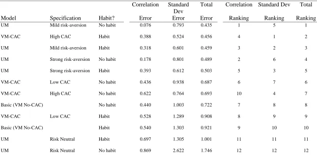
Given the differences in performance of the twelve different models across
each of the eight diagnostics considered, we construct three meta-statistics to
better understand their relative overall performance. First, for each model, we
calculate the average absolute difference between the predicted and observed
GDP. This average is termed the “Correlation Error”. We also calculate the
absolute difference between the predicted and observed standard deviation of
these variables when normalized by GDP. These are then standardized by the
observed standard deviation in each case before being averaged; this is referred to
as the “Standard Deviation Error”. The final meta-statistic, “Total Error”, for
each model is then the average of the correlation and standard deviation errors.
Results are reported in Table 2.
---
Insert Table 2 about here
---
We can see that five models perform poorly as they are in the bottom half
of all specifications for all three of the meta-statistics. Worst of all are the
utility-maximizing models when it is assumed that the firm manager is risk-neutral. The
basic model, with neither capital adjustment costs nor agency problems, also
performs poorly. Finally the habit formation, VM-CAC model with low
adjustment costs, can clearly be rejected by the data. Five other models, by
contrast, are in the top half for each of the three meta-statistics. These include all
four of the UM models with risk averse managers, and the VM-CAC model with
high capital adjustment costs and a representative household with habit formation
The three models that we have particularly shortlisted for consideration,
given their high ability to explain the correlation between dividend and GDP
growth, feature in the top three positions according to the total error statistic.
They also feature first, second on fifth on the standard deviation error statistic,
even though their ability to explain volatility was not a criterion for their
selection. From this it is clear that including either capital adjustment costs or a
value-maximizing risk-averse manager makes a material improvement on the
standard economic model across a wide range of metrics covering volatility and
covariance. For the UM model, this finding is not particularly sensitive to either
the level of risk aversion of the manager (although the low risk aversion manager
specification is preferred), or the presence or absence of household habit
formation. The UM, mild risk aversion, with habit model is perhaps of particular
note as it lies within the top three models for all of the meta-statistics considered.
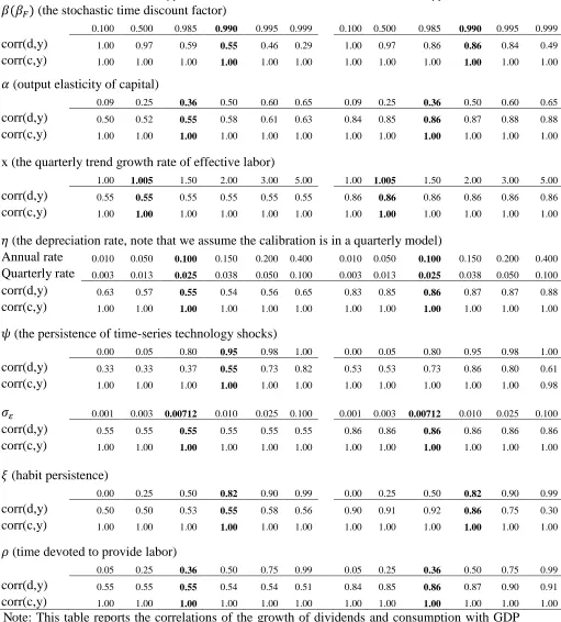
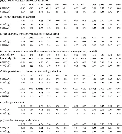
3.1 Sensitivity analysis
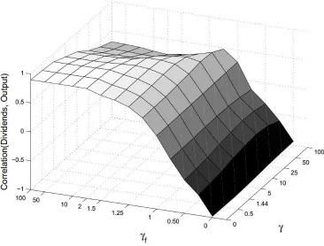
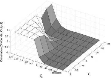
In Figures 1 and 2, we explore the sensitivity of dividend cyclicality to the choice
of and for different levels of . For the UM model, the results are largely
insensitive to . The pro-cyclicality of equity payouts declines steeply with
, but, above this level, equity payouts quickly become highly pro-cyclical at a
relatively steady level. For the VM-CAC model, there is greater sensitivity of the
of is at the lower end of standard estimates. With higher values of , an
even higher capital adjustment cost is required to explain the observed
pro-cyclicality of payout policy.
---
Insert Figures 1 & 2 around here
---
Results detailing the sensitivity of dividend and consumption
pro-cyclicality to a wide range of plausible parameter values are presented in Tables 3
(for the UM model) and 4 (for the VM-CAC model).
---
Insert Tables 3 & 4 around here
---
For the UM model with , there is relatively low sensitivity of the
correlation between dividends and output for most parameters considered ( , , ,
x, and ) and aggregate consumption is positively related to output in all cases,
with this relationship becoming stronger when the manager becomes more
risk-averse ( =5). The pro-cyclicality of dividends is, however, sensitive to the
stochastic time discount factor ( ) and the persistence of technology shocks ( ).
As expected, dividends are more pro-cyclical when technology persistence
managers. As the rate of pure time preference increases ( decreases), the
relationship between output and dividends becomes less positive.
The VM-CAC model is more sensitive to parameter choices than the UM
model. Dividends can become negatively related to output not only with low
CAC but also in the case of high CAC in the presence of relatively strong habit
persistence or low persistence of technology shocks. In addition, aggregate
dividends in the VM-low-CAC model are not as sensitive to parameter choices as
in the VM-high-CAC model. Aggregate dividends become less positively related
to output when the time discount factor, habit persistence, the elasticity of
consumption, and the depreciation rate are high and when the persistence of
technology shocks is low.
While we have been able to reconcile observed behavior with general
equilibrium using either the UM or VM-CAC models in economies without
heterogeneous agents and incomplete markets, we believe that the former is more
realistic than the latter. An estimate of is broadly consistent with
standard estimates of risk aversion. By contrast, the level of capital adjustment
cost implicit in the case is very large. Taking as an example a firm that
wishes to invest 5% of new capital into its firm: . If ,
then, from Equation 7, only makes its way into the firm and the rest
is lost to frictions. This means that only two-thirds of the money re-invested
power. Further, the explanatory power is more robust to parameter value changes
for the UM model than the VM-CAC model.
4 Concluding Remarks
In this paper we have described two general equilibrium models that explain why
external changes in the economic environment result in businesses systematically
implementing pro-cyclical equity payout policies. This resolves an anomaly that
is present in many previous general equilibrium studies. In addition, our more
sophisticated models are able to capture a number of other features of the
observed macroeconomy that are poorly captured by a basic DSGE framework.
Our preferred model is based on the assumption that managers maximize
their own objective function rather than the share price of their firms. This makes
them more reluctant to re-invest in the business in economic booms in case
conditions change. More cash can then be paid out when times are good. Even
with relatively low levels of managerial risk aversion, the calibrated theoretical
model matches the summary statistics of historical data well.
An alternative model that we have analyzed includes capital adjustment
costs within an economy where managers maximize their current share price.
These frictions also inhibit managers from heavily re-investing in a pro-cyclical
manner, and the resultant payout policy moves in line with the economy.
accurately calibrate the model in a manner that is consistent with the data and
therefore we believe this is the less credible explanation of the payout
pro-cyclicality anomaly. These findings support the idea that agency conflicts play an
important role in real business cycle models.
References
Alessandrini, F., 2003 (February). Introducing capital structure in a production economy: implications for investment, debt and dividends. Financial Valuation and Risk Management Working Paper No. 47.
Alli, K.L., Khan, A.Q., Ramirez, G.G., 1993. Determinants of corporate dividend
policy: a factorial analysis. Finan. Rev. 28, 523–547.
DOI: http://dx.doi.org/10.1111/j.1540-6288.1993.tb01361.x
An, Y., Cheung, K. 2010. Project financing: Deal or no deal. Rev. Finan. Econ. 19, 72–77. DOI: http://dx.doi.org/10.1016/j.rfe.2009.02.002
Baker, H.K., Smith, D.M., 2006. In search of a residual dividend policy. Rev. Finan. Econ. 15, 1–18. DOI: http://dx.doi.org/10.1016/j.rfe.2004.10.002
Baxer, M., King, R.G., 1999. Measuring business cycles: approximate band-pass filters for economic time series. Rev. Econ. Stat. 81, 575–593. DOI: http://dx.doi.org/10.1162/003465399558454
Bhattacharyya, N., 2007. Dividend policy: a review. Manag. Finan. 33, 4–13. DOI: http://dx.doi.org/10.1108/03074350710715773
Campbell, J.Y., 1994. Inspecting the mechanism: an analytical approach to the stochastic growth model. J. Monet. Econ. 33, 463–506. DOI: http://dx.doi.org/10.1016/0304-3932(94)90040-X
Canzoneri, M.B., Cumby, R.E., Diba, B.T., 2006 (September). How do monetary and fiscal policy interact in the European monetary union? in NBER International Seminar on Macroeconomics 2004, pp. 241–326. The MIT Press.
Carceles-Poveda, E., 2003. Capital adjustment costs and firm risk aversion. Econ. Lett. 81, 101–107. DOI: http://dx.doi.org/10.1016/S0165-1765(03)00150-2
Carceles-Poveda, E., 2005. Idiosyncratic shocks and asset returns in the real-business-cycle model: an approximate analytical approach. Macroecon. Dyn. 9, 295–320. DOI: http://dx.doi.org/10.1017/S1365100505040216
Carceles-Poveda, E., 2009. Asset prices and business cycles under market
incompleteness. Rev. Econ. Dyn. 12, 405–422. DOI:
http://dx.doi.org/10.1016/j.red.2008.07.004
Carroll, C.D., 2000. Solving consumption models with multiplicative habits. Econ. Lett. 68, 67–77. DOI: http://dx.doi.org/10.1016/S0165-1765(00)00223-8
Carroll, C.D., Overland, J., Weil, D.N., 2000. Saving and growth with habit
formation. Am. Econ. Rev. 90, 341–355. URL:
http://www.jstor.org/stable/117332
Christiano, L.J., Fisher, J., 1995. Tobin’s q and asset returns: implications for business cycle analysis. NBER Working Paper No. 5292. URL: http://www.nber.org/papers/w5292
Collard, F., Dellas, H., 2006. The case for inflation stability. J. Monet. Econ. 53, 1801–1814. DOI: http://dx.doi.org/10.1016/j.jmoneco.2005.09.002
Constantinides, G.M., 1990. Habit formation: a resolution of the equity premium
puzzle. J. Polit. Econ. 98, 519–543. URL:
http://www.jstor.org/stable/2937698
Cooper, R.W., Haltiwanger, J.C., 2006. On the nature of capital adjustment costs. Rev. Econ. Stud. 73, 611-633. DOI: http://dx.doi.org/10.1111/j.1467-937X.2006.00389.x
Danthine, J.P., Donaldson, J.B., 2002. Labour relations and asset returns. Rev. Econ. Stud. 69, 41–64. DOI: http://dx.doi.org/10.1111/1467-937X.00197
Dynan, K.E., 2000. Habit formation in consumer preferences: evidence from
panel data. Am. Econ. Rev. 90, 391–406. URL:
http://www.jstor.org/stable/117335
Gershun, N., 2010. Habit persistence, impediments to production factor adjustments, and asset returns in general equilibrium models with self-fulfilling expectations. Rev. Finan. Econ. 19, 19–27. DOI: http://dx.doi.org/10.1016/j.rfe.2009.08.001
Hansen, G.D., 1985. Indivisible labor and the business cycle. J. Monet. Econ. 16, 309–327. DOI: http://dx.doi.org/10.1016/0304-3932(85)90039-X
Heaton, J., Lucas, D., 2000. Portfolio choice and asset prices: the importance of
entrepreneurial risk. J. Finan. 55, 1163-1198.
DOI: http://dx.doi.org/10.1111/0022-1082.00244
Jermann, U.J., 1998. Asset pricing in production economies. J. Monet. Econ. 41, 257–275. DOI: http://dx.doi.org/10.1016/S0304-3932(97)00078-0
Jermann, U., Quadrini, V., 2012. Macroeconomic effects of financial shocks. Am. Econ. Rev. 102, 238–271. DOI: http://dx.doi.org/10.1257/aer.102.1.238
Kydland, F.E., Prescott, E.C., 1982. Time to build and aggregate fluctuations. Econom. 50, 1345–1370. URL: http://www.jstor.org/stable/1913386
Lang, L.H.P., Litzenberger, R.H., 1989. Dividend announcements: Cash flow signalling vs. free cash flow hypothesis? J. Finan. Econ. 24, 181–191. DOI: http://dx.doi.org/10.1016/0304-405X(89)90077-9
Ljungqvist, L. Sargent, T.J., 2004. Recursive Macroeconomic Theory. The MIT Press, Cambridge, MA.
Mehra, R., Prescott, E.C., 1985. The equity premium: a puzzle. J. Monet. Econ. 15, 145–161. DOI: http://dx.doi.org/10.1016/0304-3932(85)90061-3
Otrok, C., B. Ravikumar, B., Whiteman, C., 2002. Habit formation: a resolution of the equity premium puzzle? J. Monet. Econ. 49, 1261–1288. DOI: http://dx.doi.org/10.1016/S0304-3932(02)00147-2
Parrino, R., Poteshman, A.M., Weisbach, M.S., 2005. Measuring investment distortions when risk-averse managers decide whether to undertake risky projects. Finan. Manag. 34, 21–60. DOI: http://dx.doi.org/10.1111/j.1755-053X.2005.tb00091.x
Prescott, E.C., 1986. Theory ahead of business cycle measurement. Federal Reserve Bank of Minneapolis Quarterly Review (Fall), 9–22.
Radner, R., 1970. Problems in the theory of markets under uncertainty. Am. Econ. Rev. 60, 454–460. URL: http://www.jstor.org/stable/1815845
Sandmo, A., 1971. On the theory of the competitive firm under price uncertainty. Am. Econ. Rev. 61, 65–73. URL: http://www.jstor.org/stable/1910541
Santoro, M., Wei, C., 2011. Taxation, investment and asset pricing. Rev. Econ. Dyn. 14, 443–454. DOI: http://dx.doi.org/10.1016/j.red.2010.09.002
Fig. 1. The correlation (Z axis) between equity payouts and output growth in the
[image:30.612.128.494.113.391.2]Fig. 2. The correlation (Z axis) between equity payouts and output growth in
[image:31.612.126.498.115.376.2]Table 1
Modeled and observed summary statistics for the macroeconomy
Note: This table shows the predicted values of (i) the correlation between the growth of each variable (dividends, consumption, hours worked and investment) and GDP growth, (ii) the standard deviation of each variable, normalized by GDP and (iii) the observed value of each variable from the US economy.
a See notes to Footnote 10.
Baseline Models Advanced Specifications
US Dataa (1984:1 -2010:2) With/without habit Model type No
Habit Habit No Habit Habit
VM VM UM UM UM
VM-CAC
VM-CAC UM UM UM
VM-CAC VM-CAC Model specification No-CAC No-CAC Risk Neutral Mild risk-averse ( =1.25) Strong risk-averse ( =5) Low CAC ( =40) High CAC ( =0.30) Risk Neutral Mild risk-averse ( =1.25) Strong risk-averse ( =5) Low CAC ( =40)
High CAC ( =0.30)
(1) (2) (3) (4) (5) (6) (7) (8) (9) (10) (11) (12)
Correlation with GDP
Dividends -0.98 -0.96 -0.95 0.50 0.90 -0.98 1.00 -0.99 0.55 0.86 -0.95 0.55 0.50 Consumption 0.94 0.51 -0.85 1.00 1.00 0.96 1.00 -0.08 1.00 1.00 0.55 0.97 0.97 Hours worked 0.98 0.98 0.96 0.99 1.00 0.99 -1.00 0.97 -0.23 -0.22 0.98 -0.56 0.84 Investment 0.99 0.98 0.97 1.00 1.00 0.99 1.00 0.99 1.00 1.00 0.98 0.78 0.88 Standard deviation
Table 2
Meta-statistics on model performance
Correlation Standard Dev
Total Correlation Standard Dev Total
Model Specification Habit? Error Error Error Ranking Ranking Ranking
UM Mild risk-aversion No habit 0.076 0.793 0.435 1 5 1
VM-CAC High CAC Habit 0.388 0.524 0.456 4 1 2
UM Mild risk-aversion Habit 0.318 0.601 0.459 3 2 3
UM Strong risk-aversion No habit 0.178 0.801 0.489 2 6 4
UM Strong risk-aversion Habit 0.393 0.612 0.503 5 3 5
VM-CAC Low CAC No habit 0.436 0.938 0.687 6 7 6
VM-CAC High CAC No habit 0.622 0.764 0.693 10 4 7
Basic (VM No-CAC) No habit 0.440 1.003 0.722 7 8 8
VM-CAC Low CAC Habit 0.528 1.289 0.908 8 9 9
Basic (VM No-CAC) Habit 0.540 1.303 0.921 9 10 10
UM Risk Neutral Habit 0.697 1.305 1.001 11 11 11
UM Risk Neutral No habit 0.869 2.622 1.746 12 12 12
Table 3
Sensitivity analysis for UM model
(the stochastic time discount factor)
0.100 0.500 0.985 0.990 0.995 0.999 0.100 0.500 0.985 0.990 0.995 0.999
corr(d,y) 1.00 0.97 0.59 0.55 0.46 0.29 1.00 0.97 0.86 0.86 0.84 0.49
corr(c,y) 1.00 1.00 1.00 1.00 1.00 1.00 1.00 1.00 1.00 1.00 1.00 1.00
(output elasticity of capital)
0.09 0.25 0.36 0.50 0.60 0.65 0.09 0.25 0.36 0.50 0.60 0.65
corr(d,y) 0.50 0.52 0.55 0.58 0.61 0.63 0.84 0.85 0.86 0.87 0.88 0.88
corr(c,y) 1.00 1.00 1.00 1.00 1.00 1.00 1.00 1.00 1.00 1.00 1.00 1.00
x (the quarterly trend growth rate of effective labor)
1.00 1.005 1.50 2.00 3.00 5.00 1.00 1.005 1.50 2.00 3.00 5.00
corr(d,y) 0.55 0.55 0.55 0.55 0.55 0.55 0.86 0.86 0.86 0.86 0.86 0.86
corr(c,y) 1.00 1.00 1.00 1.00 1.00 1.00 1.00 1.00 1.00 1.00 1.00 1.00
(the depreciation rate, note that we assume the calibration is in a quarterly model)
Annual rate 0.010 0.050 0.100 0.150 0.200 0.400 0.010 0.050 0.100 0.150 0.200 0.400
Quarterly rate 0.003 0.013 0.025 0.038 0.050 0.100 0.003 0.013 0.025 0.038 0.050 0.100
corr(d,y) 0.63 0.57 0.55 0.54 0.56 0.65 0.83 0.85 0.86 0.87 0.87 0.88
corr(c,y) 1.00 1.00 1.00 1.00 1.00 1.00 1.00 1.00 1.00 1.00 1.00 1.00
(the persistence of time-series technology shocks)
0.00 0.05 0.80 0.95 0.98 1.00 0.00 0.05 0.80 0.95 0.98 1.00
corr(d,y) 0.33 0.33 0.37 0.55 0.73 0.82 0.53 0.53 0.73 0.86 0.80 0.61
corr(c,y) 1.00 1.00 1.00 1.00 1.00 1.00 1.00 1.00 1.00 1.00 1.00 0.98
0.001 0.003 0.00712 0.010 0.025 0.100 0.001 0.003 0.00712 0.010 0.025 0.100
corr(d,y) 0.55 0.55 0.55 0.55 0.55 0.55 0.86 0.86 0.86 0.86 0.86 0.86
corr(c,y) 1.00 1.00 1.00 1.00 1.00 1.00 1.00 1.00 1.00 1.00 1.00 1.00
(habit persistence)
0.00 0.25 0.50 0.82 0.90 0.99 0.00 0.25 0.50 0.82 0.90 0.99
corr(d,y) 0.50 0.50 0.53 0.55 0.58 0.56 0.90 0.91 0.92 0.86 0.75 0.30
corr(c,y) 1.00 1.00 1.00 1.00 1.00 1.00 1.00 1.00 1.00 1.00 1.00 1.00
(time devoted to provide labor)
0.05 0.25 0.36 0.50 0.75 0.99 0.05 0.25 0.36 0.50 0.75 0.99
corr(d,y) 0.55 0.55 0.55 0.54 0.54 0.51 0.84 0.85 0.86 0.87 0.90 0.91
corr(c,y) 1.00 1.00 1.00 1.00 1.00 1.00 1.00 1.00 1.00 1.00 1.00 1.00
Table 4
Sensitivity analysis for VM-CAC model
(the stochastic time discount factor)
0.900 0.970 0.985 0.990 0.995 0.999 0.900 0.970 0.985 0.990 0.995 0.999
corr(d,y) -0.42 -0.87 -0.93 -0.95 -0.97 -0.98 0.99 0.88 0.69 0.55 0.32 0.06
corr(c,y) 0.77 0.60 0.56 0.55 0.54 0.53 1.00 0.99 0.98 0.97 0.96 0.94
(output elasticity of capital)
0.10 0.25 0.36 0.50 0.60 0.65 0.10 0.25 0.36 0.50 0.60 0.65
corr(d,y) -0.89 -0.94 -0.95 -0.95 -0.95 -0.95 0.61 0.57 0.55 0.53 0.54 0.55
corr(c,y) 0.66 0.58 0.55 0.52 0.50 0.49 1.00 0.99 0.97 0.94 0.91 0.90
x (the quarterly trend growth rate of effective labor)
1.00 1.005 1.50 2.00 3.00 5.00 1.00 1.005 1.50 2.00 3.00 5.00
corr(d,y) -0.95 -0.95 -0.95 -0.95 -0.95 -0.95 0.55 0.55 0.55 0.55 0.55 0.55
corr(c,y) 0.55 0.55 0.55 0.55 0.55 0.55 0.97 0.97 0.97 0.97 0.97 0.97
(the depreciation rate, note that we assume the calibration is in a quarterly model)
Annual rate 0.06 0.10 0.15 0.20 0.40 0.60 0.06 0.10 0.15 0.20 0.40 0.60
Quarterly rate 0.015 0.025 0.038 0.050 0.100 0.150 0.015 0.025 0.038 0.050 0.100 0.150
corr(d,y) -0.96 -0.95 -0.93 -0.91 -0.84 -0.78 0.70 0.55 0.42 0.35 0.23 0.19
corr(c,y) 0.54 0.55 0.57 0.60 0.70 0.78 0.98 0.97 0.97 0.97 0.97 0.98
(the persistence of time-series technology shocks)
0.00 0.05 0.80 0.95 0.98 1.00 0.00 0.05 0.80 0.95 0.98 1.00
corr(d,y) -1.00 -1.00 -0.99 -0.95 -0.92 -0.85 -0.97 -0.93 -0.09 0.55 0.62 0.62
corr(c,y) 0.19 0.18 0.34 0.55 0.61 0.67 0.73 0.77 0.94 0.97 0.97 0.97
0.001 0.003 0.00712 0.010 0.025 0.100 0.001 0.003 0.00712 0.010 0.025 0.100
corr(d,y) -0.95 -0.95 -0.95 0.95 -0.95 -0.95 0.55 0.55 0.55 0.55 0.55 0.55
corr(c,y) 0.55 0.55 0.55 0.55 0.55 0.55 0.97 0.97 0.97 0.97 0.97 0.97
(habit persistence)
0.00 0.25 0.50 0.82 0.90 0.99 0.00 0.25 0.50 0.82 0.90 0.99
corr(d,y) -0.98 -0.96 -0.95 -0.95 -0.97 -1.00 1.00 1.00 0.96 0.55 -0.03 -0.99
corr(c,y) 0.96 0.93 0.85 0.55 0.39 0.10 1.00 1.00 1.00 0.97 0.91 0.29
(time devoted to provide labor)
0.05 0.25 0.36 0.50 0.75 0.99 0.05 0.25 0.36 0.50 0.75 0.99
corr(d,y) -0.96 -0.95 -0.95 -0.95 -0.95 -0.95 0.74 0.62 0.55 0.44 0.21 -0.20