Cleveland State University
EngagedScholarship@CSU
Electrical Engineering & Computer Science Faculty
Publications
Electrical Engineering & Computer Science
Department
12-1-2013
Scanless Fast Handoff Technique Based on Global
Path Cache for WLANs
Weetit Wanalertlak
Oregon State University, [email protected]
Ben Lee
Oregon State University, [email protected]
Chansu Yu
Cleveland State University, [email protected]
Follow this and additional works at:
https://engagedscholarship.csuohio.edu/enece_facpub
How does access to this work benefit you? Let us know!
Publisher's Statement
The final publication is available at Springer via http://dx.doi.org/10.1007/s11227-012-0805-7
This Article is brought to you for free and open access by the Electrical Engineering & Computer Science Department at EngagedScholarship@CSU. It has been accepted for inclusion in Electrical Engineering & Computer Science Faculty Publications by an authorized administrator of
EngagedScholarship@CSU. For more information, please [email protected].
Repository Citation
Wanalertlak, Weetit; Lee, Ben; and Yu, Chansu, "Scanless Fast Handoff Technique Based on Global Path Cache for WLANs" (2013). Electrical Engineering & Computer Science Faculty Publications. 290.
Scanless fast handoff technique based on global
Path-Cache for WLANs
Weetit Wanalertlak·Ben Lee·Chansu Yu·
Myungchul Kim·Seung-Min Park·Won-Tae Kim
Abstract Wireless LANs (WLANs) have been widely adopted and are more conve-nient as they are interconnected as wireless campus networks and wireless mesh net-works. However, time-sensitive multimedia applications, which have become more popular, could suffer from long end-to-end latency in WLANs. This is due mainly to handoff delay, which in turn is caused by channel scanning. This paper proposes W. Wanalertlak·B. Lee (
)School of Electrical Engineering and Computer Science, Oregon State University, Corvallis, OR 97331, USA
e-mail:[email protected] W. Wanalertlak
e-mail:[email protected] C. Yu
Department of Electrical and Computer Engineering, Cleveland State University, Cleveland, OH 44115, USA
e-mail:[email protected] C. Yu
WCU Division of IT Convergence Engineering, Pohang University of Science and Technology (POSTECH), San 31, Hyoja, Pohang, Gyeongbuk 790-784, Korea
M.C. Kim
Department of Computer Science, Korea Advanced Institute of Science and Technology (KAIST), 119 Munji-ro, Yuseong-gu, Daejeon 305-702, South Korea
e-mail:[email protected] S.-M. Park·W.-T. Kim
Electronics and Telecommunications Research Institute (ETRI), Daejeon, South Korea S.-M. Park
e-mail:[email protected] W.-T. Kim
a technique calledGlobal Path-Cache(GPC) that provides fast handoffs in WLANs.
GPC properly captures the dynamic behavior of the network and mobile stations (MSs), and provides accurate next-AP (access point) predictions to minimize the handoff latency. Moreover, the handoff frequencies are treated as time-series data, thus GPC calibrates the prediction models based on short-term and periodic behav-iors of mobile users. Our simulation study shows that GPC virtually eliminates the need to scan for APs during handoffs and results in much better overall handoff delay compared to existing methods.
Keywords Wireless LANs·Handoff·Channel scanning·Mobility prediction·
Time-series analysis
1 Introduction
Wireless communication technology together with the advancements in applications and network software allow users to be connected and be productive while on the road.Wireless LANs(WLANs) based on the IEEE 802.11 standard [12], better known
asWi-Fi hot spots, are already prevalent in residential as well as public areas, such as
airports, university campuses, shopping malls, coffee shops, etc. Moreover, numer-ous efforts have already been underway to connect Wi-Fi hot spots to offer a better connectivity over a larger geographical area such as community networks that cover metropolitan areas of major US cities [19,23,30,31].
One of the greatest benefit of Wi-Fi hot spots or community networks is mobil-ity support, which allows a user, for example, to continually talk on aVoice over IP
(VoIP) application or watch a video stream while walking or riding a bus between city blocks. However, mobility incurs a large handoff delay when amobile station
(MS) switches connection from oneaccess point(AP) to another. The key to
reduc-ing the handoff delay is to minimize thescanning process, which involves probing
all the communication channels to fin the best available AP. Recent studies found that passively scanning for APs during a handoff can take as much as 1 second [28] and actively scanning for APs requires 350–500 ms [28]. This becomes a major con-cern for mobile multimedia applications such as VoIP where the end-to-end delay is recommended to be not greater than 50 ms [9].
Since the scanning process represents more than 90 % of the overall handoff delay, a number of techniques have been proposed to specificall optimize the scanning process [6,32,33,41]. These methods employ extra hardware, either in the form of additional radios [6] or an overlay sensor network [41] to detect APs, selectively scan channels based on topological placements of APs [32], and predict the next point-of-attachment based on signal strength [33]. Unfortunately, these techniques neither provide next-AP predictions that can eliminate the need to scan for APs nor consider the mobility patterns of MSs, which are dictated by the structure of a building or a city block and the past behaviors of MSs. There are also methods that consider mobility history of MSs to provide next-AP predictions [36]. However, these methods tend to be general and thus they do not consider the special characteristics of WLANs, such as highly overlapped cell coverage, MAC contention, and variations in link quality.
In [42], we presented a solution, called theGlobal Path-Cache(GPC) technique,
which eliminates the need to perform scanning for available APs and thus results in faster handoffs. The key idea of GPC is to predict the next point-of-attachments based on the history of mobility patterns of MSs. This is achieved by maintaining the handoff history of all the MSs in the network, and then monitoring an MS’s di-rection of movement relative to the topological placement of APs to predict its next point-of-attachment. In addition, next-AP predictions are based on the frequencies of occurrences rather than signal strength. Therefore, it takes into consideration that mobility patterns are dictated by the structure of a building or a city block and the past behaviors of MSs. The GPC technique is an adaptive algorithm, which is independent of topological placements of APs and the number of channels used.
This paper extends our earlier work on GPC by also considering short-term hand-off behaviors and significantl expanding its evaluation. Therefore, in addition to providing a discussion of the basic GPC scheme, the specifi contributions of this paper are as follows:
– First, the basic GPC scheme presented in [42] provides next-AP predictions based on long-term frequency of handoffs and is unable to capture short-term and peri-odic handoff behaviors that are crucial for improving the prediction accuracy for all scenarios. This paper enhances the basic GPC scheme by treating the handoff frequencies as time-series data, thus GPC calibrates the prediction models based on specifi characteristics of WLAN by applyingAutoRegressive Integrated Moving Average(ARIMA) andExponential Weighted Moving Average(EWMA).
– Second, performance evaluation is significantl expanded to include a much larger network (i.e., MetroFi Portland [19]), and analyze the performance effects of dif-ferent types of users and the improvements provided by the time-series analysis.
Our simulation study shows that the basic GPC scheme results in superior handoff delay compared toSelective Scan with Caching(SSwC) [33] andNeighbor Graph
(NG) [32]. The time-series based GPC scheme further improves the average 1st next-AP prediction accuracy by as much as 17.1 % and reduces the handoff latency as much as 8.5 % compared to the basic GPC scheme. Moreover, the handoff latency improvements for some groups of MSs are as high as 15.1–27.1 %.
The paper is organized as follows. Section2presents the background of the IEEE 802.11 handoff procedure. Section3discusses the related work. Section4discusses the basic GPC technique. Section5presents the time-series based prediction model for GPC. Section6evaluates the performance of the proposed method. Finally, Sect.7
concludes the paper and discusses future work.
2 Background—scanning process in IEEE 802.11
In the IEEE 802.11 standard, when an MS moves from one cell to another, the net-work interface senses the degradation of signal quality in the current channel. The signal quality continues to degrade as the MS moves further away from the current AP, and the MS initiates a handoff to a new cell when the signal quality reaches a preset threshold [32]. This process starts scanning for new cells using either passive
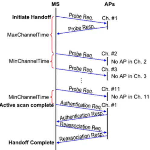
Fig. 1 Active Scanning in IEEE 802.11
or active scanning. Inpassive scanning, MS switches its transceiver to a new channel
and waits for a beacon to be sent a new AP, typically every 100 ms, or until the wait-ing time reaches a predefine maximum duration, which is longer than the beacon interval. Moreover, the time MS has to wait varies since beacons sent by APs are not synchronized. For these reasons, a recent study has shown that MSs can spend up to 1 second to scan all possible channels [28], which results in unacceptable handoff delay.
Inactive scanningshown in Fig.1, an MS broadcasts a probe request and waits
for a response. If the MS receives a response from an AP, it assumes there may be other APs in the channel and waits forMaxChannelTime. Otherwise, the MS only
waits forMinChannelTime. MinChannelTime is shorter than MaxChannelTime to
keep the overall handoff delay low, but it should be long enough for MS to receive a possible response. A typical duration for scanning each channel is around 25 ms and 350–500 ms for all 11 channels [28].
After scanning, MS typically joins the network with the strongest signal strength, which is done by performing authentication and association/reassociation. Authen-tication is the process that an MS uses to announce its identity to the new AP. In the IEEE 802.11 standard, authentication is performed using open system or shared key. Open system authentication is the default method for IEEE 802.11, and involves the MS sending authentication request frame, which contains source address in the frame header and information in the frame body to indicate the type of authentica-tion, to the AP. Then, the AP sends the authentication response frame back to the MS. This frame has the authentication result and the information to indicate the type of authentication.
The next step is association/reassociation, which allows the distribution system to keep track of the location of each MS so frames destined for the MS can be for-warded to the correct AP. How association/reassociation requests are processed is implementation-specific but typically involves allocation of frame buffers and, in the case of reassociation, communicating with the old AP so that any frames buffered at the old AP are transferred to the new AP and the old AP terminates its association with the MS. Finally, the last step involves the new AP updating the Ethernet Address
Table in the switch that connects both the old and the new APs so that the network traffi can be rerouted.
3 Related work
3.1 Mobility prediction
Mobility prediction is crucial for mitigating the effects of handoffs and therefore improving QoS. There has been a plethora of work on mobility prediction for a variety of wireless networks, such as cellular [1,14,16,35,44,45], WLANs [8,10,15,24,
26,33,36], sensor networks [47] ad hoc networks [38], and wireless mesh networks [3,13], and applied to reduce handoff latency [24,33], minimize handoff frequency [15], provide efficien resource reservation [1,14,16,35,36,44,45], improve routing protocols [38], and conserve power [47].
Although many different mobility prediction techniques have been proposed, these techniques can be broadly classifie into the following three categories. First, data-miningtechniques use a database to track and characterize the long-term mobility
patterns of MSs, which are then used to predict their locations to reduce the sig-naling overhead during handoff [14, 44, 45]. Second, topology-based techniques
use the knowledge of geographical locations of APs and directional movement of MSs [10,35]. Third,stochastictechniques provide mobility predictions using
prob-abilistic models. These techniques apply the knowledge of geographic coordinates of MSs from either GPS or triangulation of signal strengths to predicted future loca-tions [1,16].
Although all these techniques provide mobility prediction in cellular networks, they are not efficien solutions for WLANs. For example, data-mining techniques re-quire large storage and fast processors to analyze long-term mobility behavior. In ad-dition, the latter two techniques typically require a GPS device to obtain information about locations and directions of MSs. For systems that rely on signal triangulation, including methods for WLANs [26], their effectiveness may be limited due to the fact that WLANs are mainly used for indoors and crowded outdoor areas where the sig-nal strength is highly affected by interference rather than distance [29]. The technique closest to ours is Markov-based mobility predictions, which rely on the fact that the probability of the future outcome is based on the current and past outcomes [8,37]. Typically, a Markov mobility predictor maintains a collection of past locations of MSs and predicts future locations of MSs based on the value of conditional probabil-ity that matches with the past locations of MSs. The Markov-based technique can be found in many mobility-prediction algorithms, including ours. However, the proposed GPC scheme is designed to work seamlessly with the 802.11 MAC layer protocol and can be used to enhanced these methods by considering short-term mobility patterns using time-series analysis.
3.2 Reducing handoff delay in WLANs
There has been a lot of work done to reduce the handoff delay in WLANs. The re-lated work discussed here focuses on optimizing the probing or scanning process,
which is the most time-consuming part of a handoff [20,40].MultiScanuses an extra
WLAN network interface to opportunistically scan and pre-associate with alternative APs to avoid disconnections [6]. The basic idea is to have the firs WLAN interface communicate with the current AP while the second WLAN interface scans for new APs. This scan information is then used to connect to the new AP before the con-nection is lost from the current AP. A similar technique calledMake-Before-Break
also uses two WLAN cards, but allows the card that scanned the channels to also perform authentication and association to eliminate MAC layer handoff delay [27]. In contrast,LeapFrog uses an extra WLAN interface on the AP side to broadcast
beacon messages across all the channels.Selective Active Scanninguses an overlay
sensor network to obtain information on the presence of APs and the quality of their transmission channels [41]. This way, an MS can broadcast an AP-list request to sur-rounding sensor nodes to obtain a precise information about neighboring APs, and initiate a scanning process solely based on this list. Although these techniques can provide fast handoffs, they require extra hardware, implemented either on the client side, AP side, or as a separate control plane, which may be impractical and/or power-inefficient The proposed GPC method requires only one WLAN card.
Another technique to reduce the handoff delay is to either passively or actively scan for available APs in the background.SyncScanis a passive method that requires
APs to send staggered periodic beacons to allow an MS to scan for additional APs while it is still connected to the current AP [28]. InSmooth Handoff, an MS actively
scans for APs in multiple sub-phases with data transmission in-between sub-phases [17]. Although the handoff delay or packet loss can be reduced, there is a hidden cost since an MS has to occasionally suspend its communication to either listen or partially scan for other APs. Nonetheless, the GPC method proposed in this paper is an orthogonal approach to the background scanning and thus they can be deployed together to reduce the cost of performing a full scan.
Other methods that are closest to ours in terms of reducing the scanning delay areNeighbor Graph[32],Pre-Authentication Path[24],Selective Scan with Caching
[33],Enhanced FastScan[26], andDirection Handoff[10]. The Neighbor Graph and
Pre-Authentication Path techniques reduce the number of channels to scan by defin ing a directed graph that represents the topological placement of APs and the mobility patterns of MSs. Moreover, edges between APs represent handoffs that are added or deleted to reflec the changing conditions. In addition, the Pre-Authentication Path technique reduces the signaling overhead between MS and AP by allowing MSs to pre-authenticate and pre-reassociate with APs within a directed graph before the ac-tual handoff occurs. Although both of these techniques significantl reduce the aver-age number of channels probed, they do not provide next point-of-attachment predic-tions and thus all active edges (i.e., adjacent channels) emanating from a node need to be scanned.
Selective Scan with Caching minimizes the need to scan during a handoff by pre-dicting next point-of-attachment based on signal strength. An MS joining the network for the firs time performs a full scan. Then, the corresponding bits in the channel mask are set for all the probe responses received from APs, as well as bits for chan-nels 1, 6, and 11 with the premise that these chanchan-nels are more likely to be used by APs. As MS connects to the AP with the strongest signal, the corresponding bit in
the channel mask is reset based on the assumption that the likelihood of adjacent APs having the same channel is very small. In addition, two other APs’ addresses repre-senting the second and third strongest signals are stored in theAP-cacheusing the
current AP’s address as the key. These two APs represent the best and second-best candidates for subsequent handoffs. During the next handoff, the MS will attempt to reassociate with these two APs in order. If it fails to reassociate with both APs or an entry is not found in the AP-cache, a selective scan is performed based on the channel mask to choose two additional APs with the strongest signals and stores them in the AP-cache. If no APs are discovered with the current channel mask, bits in the channel mask are inverted and another scan is performed. If the partial scan fails to discover APs, a full scan is performed. However, in order to use the information from the last scanning period for the current handoff, the direction of MS movement relative to the cell layout must be identical to the one in the last handoff. This is often not the case and thus the AP-cache will frequently fail to provide correct next-AP predictions.
Enhanced FastScan (EFS) reduces scanning delay by restricting the number of candidate APs to scan based on the predicted location of an MS. EFS divides the coverage area of the current AP into four areas: NE, NW, SE, and SW. To determine the area where MS is located, Wi-Fi Positioning System (WPS) is used, and the co-ordinates of APs are added to beacon frames. However, WPS requires a large amount of scanned data to be processed, which is time-consuming, and as stated before WPS may not provide accurate location information due to interference. The Directional Handoff scheme predicts the direction of an MS using a geomagnetic sensor and thus limits the number of APs to scan. However, automatic construction of an AP table is still an issue, and the number of APs to scan will increase when a predicted direction has many APs.
Recently, there has been a growing interest in expanding the coverage area of WLANs using wireless mesh networking. InSMesh[2], multiple APs are used to
monitor the connectivity quality of MSs in their vicinity to coordinate which one of them should serve the client. This is achieved by having each MS associate with a unique multicast group of mesh nodes that are in the vicinity of the MS and the mesh node with the best connectivity to the MS sends a gratuitous ARP message to force a handoff. In contrast, the proposed GPC technique is an MS-initiated handoff method, which does not require the overhead of maintaining multicast groups. More-over, monitoring the signal quality of MSs requires all APs to be operating in the same channel and thus limiting the range of coverage area.
4 The basic GPC technique
GPC tracks past associated APs and then use this information to perform mobility predictions to reduce the handoff delay. This virtually eliminates the need to scan channels when MSs move through the coverage area with the same set of APs. This section starts off with the discussion of the basic GPC method that prioritizes multiple next-AP predictions based simply on frequency of handoff sequences. Then, Sect.5
discusses the application of time-series analysis on handoff occurrences to formulate a better model to improve the next-AP prediction accuracy.
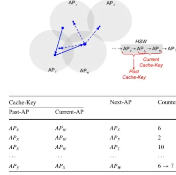
Fig. 2 Local history using HSW fork=3
Table 1 Global History in the
Path-Cache for Fig.2 Cache-Key Next-AP Counter
Past-AP Current-AP APx APw APx 6 APx APw APy 2 APx APw APz 10 · · · · APy APx APw 6→7
In order to illustrate the motivation behind GPC, Fig.2 shows an example of a coverage area that contains four APs. As the MS moves away fromAPw, it is unclear which AP it will associate with next since there are three possible candidates (i.e.,
APx,APy, orAPz). Therefore, the history of handoff sequences is maintained and used to predict the behavior of future handoffs.
In order to keep track of an MS’s handoff sequence, alocal historyis maintained
using ak-entryHandoff-Sequence Window(HSW) containing information of the
cur-rent AP as well ask−1 past-APs (i.e., the MAC address and the channel number).
Figure2illustrates HSW fork=3. An MS joining the network for the firs time has
no local history and thus its HSW contains null entries. When the MS associates with an AP, its information is queued in HSW. During each subsequent handoff, the MS sends to the server aPath-Cache requestcontaining HSW as part of an authentication
request.
When the server receives Path-Cache requests from MSs, aglobal historyof all the
handoffs in the network is maintained in thePath-Cache, where each entry contains
aCache Keyrepresented byCurrent-APandk−2past-APs,next-AP, and acounter
indicating the number of hits on this entry. Table1shows the partial content of the Path-Cache for Fig.2.
The following operations are performed when the server receives a Path-Cache request:
• Path-Cache update—The server uses thepast cache-keyrepresented by the
hand-off sequence AP0,AP1, . . . ,APk−2 in HSW to search in the Path-Cache for a matching Cache-Key. If a match is found, a check is made to see ifAPk−1 also matches the next-AP entry. If it matches, the server increments the counter for that entry by one (see Table1). If the server does not fin a match, it means the HSW is
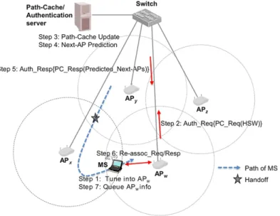
Fig. 3 The steps in the GPC technique
new. Therefore, the server stores the new handoff sequence in the Path-Cache and initializes its counter to one.
• Next-AP Prediction—The server uses thecurrent cache-key represented by the
handoff sequenceAP1,AP2, . . . ,APk−1in HSW to search in the Path-Cache for a matching Cache-Key. If a match or multiple matches are found, the server sends to MS aPath-Cache responsewith aprediction list containing a set of next-AP
predictions sorted in descending order of their counter values as part of an authen-tication response. Otherwise, a null next-AP prediction is sent back to notify of a Path-Cache miss. If the HSW in the Path-Cache request is null, it indicates the MS is joining the network for the firs time. Therefore, the server uses a special handoff sequencenull1,null2, . . . ,APtuned-in, whereAPtuned-inrepresents the current AP
the MS is tuned into, to search in the Path-Cache.
Note that the size ofkdepends on the complexity of the network topology and the
building structure. If the coverage area is small and yet there are many APs, a longer handoff history will be preferred. However, our study shows that in generalk=3 is
sufficien to provide a good next-AP prediction (see Sect.6.3). In addition, all the Path-Cache entry counters are periodically decremented to prevent saturation.
The algorithm for the GPC technique is illustrated in Fig.3, where both the Path-Cache and the Authentication server are assumed to be collocated. Each MS main-tainscurrentandfutureprediction lists. An MS performs a handoff based on the
cur-rent prediction list received from the server during the previous handoff and receives the future prediction list for the future handoff. For example, the MS in Fig.3 per-forms a handoff fromAPxtoAPwbased on the prediction list received during handoff fromAPytoAPx. Also, note that Path-Cache requests/responses are piggy-backed on authentication requests/responses. Therefore, no extra messages are needed.
Step 0: MS selects the firs element from the current prediction list as the next-AP prediction.
Step 1: MS directly tunes into the AP provided by the AP prediction. If next-AP prediction is null, MS performs a full-scan and tunes into the next-AP with the strongest signal. If the end of the current prediction list is reached, MS performs a partial scan of channels not in the current prediction list and tunes into the AP with the strongest signal.
Step 2: MS sends authentication request,Auth_Req, containing Path-Cache request, PC_Req(HSW), to the server to obtain the future prediction list for the future
handoff.
Step 3: If authentication is successful, the server performs Path-Cache Update based on the received HSW. Otherwise, authentication will time out and MS chooses the next element in the current prediction list as the next AP-prediction and proceeds to Step 1.
Step 4: The server performs Next-AP Prediction based on the received HSW and generates the future prediction list for the future handoff (i.e., fromAPwtoAP?). Step 5: The server sends authentication response, Auth_ Resp, containing
Path-Cache response with the future prediction list,PC_Resp(Predicted_Next-APs),
to the MS.
Step 6: MS sends reassociation request to the AP and receives reassociation re-sponse. If no reassociation response is received, MS selects the next element in the current prediction list as the Next-AP Prediction and proceeds to Step 1. Step 7: Information of the new AP is queued in HSW, and the future prediction list
becomes the current prediction list.
If a Path-Cache request hits on the Path-Cache and its 1st next-AP prediction is successful, GPC will reduce the overall handoff delay down to only the time required for MS to perform a channel switch plus authentication and reassociation. With each additional next-AP misprediction, the overall handoff delay increases incrementally by the channel switching time plus authentication timeout period. For example, MS firs tunes into and sends an authentication request to the firs predicted next-AP and waits for an authentication response. If the authentication times out, i.e., the 1st next-AP prediction fails, then it tunes into the second predicted next-next-AP and sends an authentication request. This process repeats until one of the predictions in the next-AP prediction list provides the correct prediction.
If either a Path-Cache miss occurs or all of the next-AP predictions fail, MS will revert back to the conventional handoff requiring a full scan. This happens when a handoff sequence is encountered for the firs time. Afterwards, the new handoff sequence will be recorded in the Path-Cache and all MSs can benefi from this infor-mation to provide fast handoffs. Therefore, as long as the Path-Cache is up to date, no scanning is necessary since one of the predictions in the next-AP prediction list will provide the correct prediction.
Note that the discussion of GPC thus far has been based on a centralized scheme. However, GPC can also be implemented using a distributed scheme where each AP maintains its own portion of the global Path-Cache. This can be achieved by relaying Path-Cache requests using reassociation requests. For example, consider again the
handoff betweenAPx andAPw shown in Fig.3. After authentication, MS sends re-association request containing the Path-Cache request toAPw. Then,APw performs Next-AP Prediction and returns the Path-Cache response as a part of the reassocia-tion response. Finally,APw sends HSW as a part of eitherInter-Access Point
Pro-tocol(IAPP) [11] or a vendor-specifi protocol to APx. AfterAPx receives HSW, Path-Cache Update is performed. This allows MSs handing off fromAPx to obtain the proper next-AP prediction list.
5 Time-series based prediction model for GPC
The previous section discussed how the basic GPC scheme uses the handoff history to effectively predict next-APs. However, the returned next-AP predictions are priori-tized based on long-term frequency of handoff sequences using counters. These coun-ters are unable to capture short-term handoff behaviors that are crucial for improving next-AP predictions for all scenarios. This is addressed by treating the frequency of handoff sequences as time-series data usingAutoRegressive Integrated Moving Aver-age(ARIMA) and its simpler formExponential Weight Moving Average(EWMA).
5.1 ARIMA based prediction model for GPC
ARIMA is known to work well for non-stationary processes [5,34], and has been used to model automotive traffi fl w [43,48] and mobility prediction [1,16]. The frequency of a handoff sequencezis treated as time-series data where the discrete
time intervaltis one minute. This archival data series can be aggregated to generate
longer time intervals as needed. The observation time period for handoff sequences
Tdepends on the system under study. For a typical WLAN environment, such as the
one shown in Fig.10, the recommended period will be at least one day to capture all possible trends within a day.
The order of an ARIMA model is denoted by the notation ARIMA(p,d,q), where p,d, andq refer to the order of theautoregressive, thedifferencing, and themoving averageparts of the model, respectively. In general, ARIMA(p,d,q) can be define
as 1−φ1B−φ2B2− · · · −φpBp ∇dz t= 1−θ1B−θ2B2− · · · −θqBq εt, (1) whereztis the observed data (i.e., frequency of handoff sequence) during the current time periodt,φis the autoregressive parameter,θ is the moving average parameter, B is thebackshiftoperator define byBmzt =zt−m,∇ is the backward difference operator of the form of∇d=(1−B)d, andε
tis the error terms.
There are two steps involved in formulating the ARIMA model. The firs step is themodel identificationthat determines the parametersp,d, andq. The second step
is themodel estimationthat determines the parametersφ andθ using an estimator
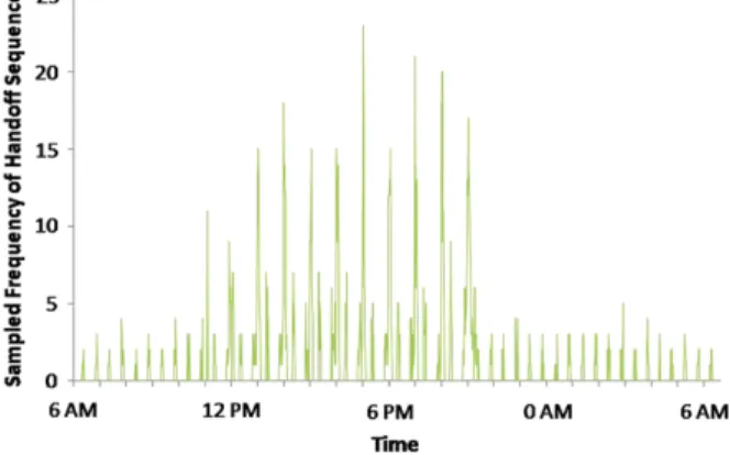
algorithm. These two steps will be illustrated using the time-series plot of frequency of handoff sequence shown in Fig.4, which was collected from simulation of user mobility in Fig.10(a) for the handoff sequenceAP4→AP5→AP6during a 24-hour period (see Sect.6.1). As can be seen, the figur shows an academic environment
Fig. 4 Sampled frequency of handoff sequencezfor
AP4→AP5→AP6in KEC
where there are more handoff activities between 11 AM and 9 PM than 10 PM and 10 AM. Moreover, these plots are characterized by extremely high fluctuation and sharp peaks during each hour exemplifying bursts of handoff activities based on class schedule.
The model identificatio begins with determining whether or not the time-series data is stationary. A stationary time-series data has no trend or seasonality. If not, the differencing transforms the time-series data to become stationary. Some time-series data may require additional differencing, but a typical value for d ranges from 0
to 2. As will be explained shortly, our analysis of the time-series data in Fig.4 be-comes stationary after the second differencing, therefore the parameterd is define
as 2. Onced is set,∇dzt in Eq. (1) is replaced by a stationary time-series dataxt, and ARIMA(p, d, q)can be rewritten as a generalAutoRegressive Moving Average
(ARMA) model shown below: 1−φ1B−φ2B2− · · · −φpBp xt= 1−θ1B−θ2B2− · · · −θqBq εt. (2) The next step in the model identificatio is to calculateautocorrelation function
(ACF) andpartial autocorrelation function(PACF) ofxt to determine the autoregres-sive (p) and moving average (q) parts of ARMA(p, q). In general, ACF at laghis
given as
ACF(h)=corr(xt, xt+h), (3) wherecorr()is thecorrelationfunction define as the ratio ofcovariance,cov(), and
variance,σ2: corr(xt, xt+h)= cov(xt, xt+h) σx2 t =E[(xt−μ)(xt+h−μ)] E[(xt−μ)2] , (4)
whereμis the mean. On the other hand, PACF at laghis define as
PACF(h)=
corr(x0, x1), h=1
corr(x0−x0h−1, xh−xhh−1), h≥2
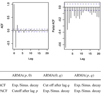
Fig. 5 ACF and PACF of the transformed time-series dataxt
in Fig.4
Table 2 Behavior of ACF and
PACF for the ARMA model ARMA(p,0) ARMA(0, q) ARMA(p, q)
ACF Exp./Sinus. decay Cut off after lagq Exp./Sinus. decay
PACF Cutoff after lagp Exp./Sinus. decay Exp./Sinus. decay
wherex0h−1andxhh−1are estimated from the(h−1)th-term linear regression model
[34].
Figure5shows the ACF and PACF plots for the transformed time-series dataxtof Fig.4. First, the ACF pattern indicatesxt is stationary since it cuts off fairly quickly. In contrast, ACF values for non-stationary data have very slow decay patterns. The parametersp andq of ARMA(p,q) can be determined by examining the plots for
ACF and PACF and applying the criteria define in Table2. For example, ARMA(0,
q) is chosen when the ACF values cut off after lag q and the PACF values have
exponential or sinusoidal decay. On the other hand, ARMA(p, 0) is chosen when
the ACF values have exponential or sinusoidal decay and the PACF values cut off after lagp. Finally, ARMA(p,q) is chosen when both ACF and PACF values have
exponential or sinusoidal decay. Based on Fig.5and the criteria define in Table2, the parametersp andq are identifie as 0 and 2, respectively. Therefore, the
time-series data in Fig.4 can be modeled as ARIMA(0, 2 ,2), which can be rewritten as
∇2zt=(1−θ1B−θ2B2)εt. (6)
We then substitute theone-step-ahead forecast errorsεt =zt− ˆzt [5], wherezˆt represents the predicted frequency of handoff sequence during the time periodt, and ∇ =(1−B), to obtain
ˆ
zt=(2−θ1)zt−1−(1+θ2)zt−2+θ1zˆt−1+θ2zˆt−2. (7) Therefore, the predicted frequency of handoff sequence during the time periodt+1, ˆ
zt+1, can be written as ˆ
wherezt andzt−1are the current and previous sampled frequencies of handoff se-quences,zˆt andzˆt−1are the current and previous predicted frequencies of handoff sequences, andθ1andθ2are parameters.
After the prediction model is defined the model estimation determines the param-etersθ1andθ2. This step typically involves curve fitting which can be done in many
different ways. The method used in our simulation isMaximum Likelihood Estimator
(MLE). In general, MLE is given by
L(β)= n t=2
f (xt|xt−1. . . x1) (9) wherexis Gaussian,βis a vector of parametersφandθ, andf (xt|xt−1. . . x1)is a conditional density function. The MLE method estimatesβ by findin the value of β that maximizes L(β). Using a graphical method that searches for the maximum L(β), the parametersθ1andθ2are estimated as 1.9783 and−0.9784, respectively.
Thus, the prediction model of the handoff sequenceAP4→AP5→AP6is given by
ˆ
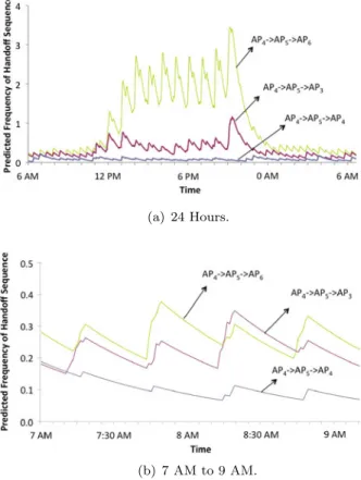
zt+1=0.0217zt−0.0216zt−1+1.9783zˆt−0.9784zˆt−1 (10) Figure 6 shows the plot of predicted frequencies for the three handoff se-quences, AP4→AP5→AP6,AP4→AP5→AP3, and AP4→AP5→AP4, us-ing the ARIMA model. This figur shows that in general the handoff sequence
AP4→AP5→AP6 occurs the most often. The major advantage of GPC based on ARIMA is that it can better track the short-term changes in the mobility pat-tern. They occur when the frequencies of handoff sequences are relatively close to-gether as in Fig. 6(a) between 0 AM and 11 AM. For example, Fig. 6(b) shows a magnifie view of the frequency of handoff sequences between 7 AM and 9 AM of Fig. 6(a). The ARIMA model is able to determine that the frequency of handoff sequenceAP4→AP5→AP3overtakes the frequency of handoff sequence AP4→AP5→AP6and becomes the highest around 8:20 AM. Even a small increase
in handoff activities can cause the mobility prediction to change. Therefore, ARIMA-based GPC correctly providesAP3as the 1st next-AP prediction. However, the basic GPC scheme based only on long-term history cannot capture these short-term varia-tions causing mispredicvaria-tions.
5.2 EWMA based prediction model for GPC
EWMA is equivalent to ARIMA(0,1,1)[34,43] and is much simpler to formulate
than the general ARIMA model. EWMA can be define as
ˆ
zt+1=(1−λ)zˆt+λzt (11)
whereλis the smoothing factor (0< λ <1). The parameterλdetermines the
char-acteristic of the EWMA model and is typically chosen experimentally. Based on our analysis,λfor the time-series data representing frequency of handoff sequences in
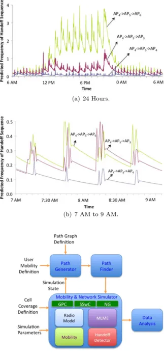
Fig.10(a) is chosen to be 0.1. Figure7(a) shows the plot of Fig.6(a) based on the EWMA model. Figure7(b) shows that EWMA, despite some noise, is also able to
Fig. 6 Predicted frequency of handoff sequenceszˆfor
AP4→AP5→AP6,
AP4→AP5→AP3, and
AP4→AP5→AP4based on
ARIMA(0, 2, 2) for KEC
capture the fact that frequency of handoff sequenceAP4→AP5→AP3becomes the highest around 8:15 AM. Although EWMA does not rely on the full statistical anal-ysis to estimate the order and the coefficients our simulation results show that this simple model gives results that are relatively close to the ones from ARIMA.
6 Performance evaluation
This section presents the performance evaluation of the proposed GPC technique. Section6.1describes the simulation environment as well as the various components of the simulator. Section6.2discusses the delay parameters used in the study. Sec-tion6.3 compares the results of the basic GPC scheme against theSelective Scan with Caching(SSwC) [33] andNeighbor Graph(NG) [21,32] techniques, as well as
presents the performance improvement using the ARIMA and EWMA models. 6.1 Simulation environment
In order to accurately simulate mobility patterns and handoffs, we developed a sim-ulator that implements a WLAN radio model, generates realistic mobility patterns based on building and city layouts, and supports management frames needed to im-plement scanning, authentication, and reassociation. The structure of the simulator is
Fig. 7 Predicted Frequency of Handoff Sequences based on EWMA for KEC
Fig. 8 Simulation model
shown in Fig.8, which consists of Path Generator, Path Finder, Mobility & Network Simulator, and Data Analysis modules.
ThePath Generatorgenerates a new destination waypoint based on the Path Graph
definition User Mobility definition and the current Simulation State for each MS that has completed its trip between the original and destination waypoints. ThePath Graphdefinitio is a graphical representation of all the possible paths MSs can
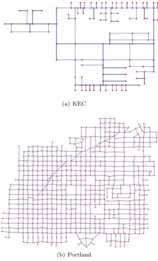
tra-Fig. 9 Paths graphs for Fig.10
verse within a simulated area, which is similar to the ones proposed in [39,46]. Fig-ure9shows the path graphs for the two network topologies used in the simulation study—KEC and Portland in Fig.10. They consist of vertices representing waypoints and segments representing paths between adjacent waypoints. TheUser Mobility
de-fine the number of MSs and APs, as well as how MSs move, including when and where an MS moves to and how long it stays at a waypoint. TheSimulation State
define the current time and the locations of all the MSs in the simulated network area. The Path Generator uses these two definition together with the current state of the simulator to randomly select destination waypoints based on amodifiedRandom
Waypoint model [7,22]. Our modifie Random Waypoint model allows a probabil-ity distribution to be assigned to sub-areas or regions within a path graph based on different groups of MSs at different times. ThePath Finder module then uses the
path-finde algorithm [25] to generate the shortest path between the source and des-tination waypoints. The resulting path consists of multiple segments, which are then fed to theMobility & Network Simulator.
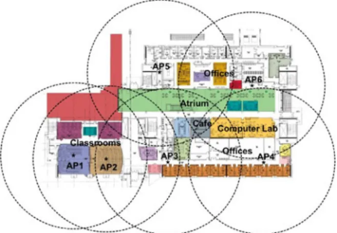
Fig. 10 Example of WLAN coverage areas
The Mobility & Network Simulator consists of Mobility module, Radio Model, Handoff Detector, and MAC subLayer Management Entity (MLME). TheMobility
module simulates the movements of MSs on the segments at one-meter resolution. TheHandoff Detectormonitors each MS’s movement, and based on theCell Cover-agedefinitio and theRadio Model, which is based on log-distance path loss model
[29], performs a handoff when the distance between the MS and the associated AP reaches the maximum radius of the coverage area. The handoff is performed using
MLMEmodule, which supports beacons, probing, authentication, and reassociation.
Finally, theData Analysismodule records the number of channel switches, the
num-ber of times MS has to wait fortmax,tmin,tauth, andtassoc(see Sect.6.2).
The two network topologies simulated are shown in Fig.10, which consists of the firs floo of the four-story, 153,000-ft2Kelley Engineering Center (KEC) at Oregon
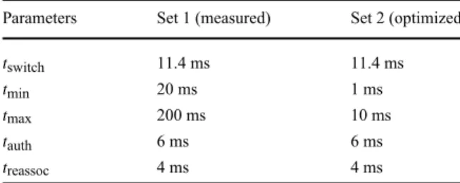
Table 3 Delay parameters used
in the simulation Parameters Set 1 (measured) Set 2 (optimized)
tswitch 11.4 ms 11.4 ms
tmin 20 ms 1 ms
tmax 200 ms 10 ms
tauth 6 ms 6 ms
treassoc 4 ms 4 ms
State University, and MetroFi, which is a public WLAN service that covers 2.5-mile2 area of Portland, Oregon [19]. The APs in KEC are connected by Ethernet switches, while APs in the MetroFi network are interconnected by a wireless mesh network [13].
The simulated coverage area for KEC contains 6 APs and 450 MSs, while the coverage area for Portland contains 40 APs and 4500 MSs. There are three groups of users in KEC: 200 students, 200 graduate students, and 50 staff members, with each having different types of mobility behaviors. For example,studentsin Fig.10(a)
mostly move between the atrium, the cafe, and the computer lab. In addition, students move in and out of the classrooms during the last ten minutes of each class hour between 8 AM and 6 PM. In contrast,graduate studentsmainly move between their
offices the atrium and the computer lab. Finally,staff moves mainly between their
office and the atrium.
The results for Portland were generated based on nine different groups with each group consisting of 500 users.Nomadicrepresents a group of MSs that can move
anywhere within the simulated area. The next four groups representcommuters(C)
who work in each of the four quadrants or regions, i.e., C-I C-II, C-III, and C-IV in Fig.10(b), which are likely to travel long distances (i.e., 15–20 blocks) to work. Moreover, these groups of MSs only move between 6 AM and 10 AM and between 6 PM and 10 PM. The last four groups representresidents(R) who live in each of the
four regions, i.e., R-I, R-II, R-III, and R-IV in Fig.10(b). These groups of MSs can move anytime but are likely to only move within few blocks (5–10 blocks) from their homes.
6.2 Simulation delay parameters
The delay parameters used in the simulation are shown in Table3:Channel Switch-ing Time(tswitch) is the time required to switch from one channel to another; Min-ChannelTime(tmin) is the minimum amount of time an MS has to wait on an empty
channel;MaxChannelTime(tmax) is the maximum amount of time an MS has to wait
to collect all the probe responses, which is used when a response is received within MinChannelTime;Authentication delay/timeout(tauth) is the time required to perform
authentication based on MAC addresses; andReassociation delay(tassoc) is the time
required to perform reassociation.
The Parameter Set 1 represents the current off-the-shelf NICs, and was obtained using an experimental setup that consisted of two laptops with PCMCIA 802.11a/b/g NICs based on Atheros AR 5002X chipsets [4] (running Linux 2.6 on Laptop #1
as a traffi generator and FreeBSD 6.1 on Laptop #2 as a traffi observer), a Sun SPARC Server with Ethernet LAN NIC (running SunOS 5.1), and an HP ProCurve Wireless Access Point 420. The NICs on the AP and on both laptops are operating on Ch. 1. Measurements were obtained by having the firs laptop transmit a stream of 16-byte UDP packets to the server, while tcpdump running on the second laptop sniffs the traffic The timetswitchwas determined by forcing the NIC on the firs laptop to
switch to Ch. 2, which has no APs, and then immediately switch back to Ch. 1. The observed time between the last UDP packet and the probe request from the firs lap-top was 22.8 ms, which represents 2·tswitch, and thustswitchis assumed to be 11.4 ms.
The timetauth was determined by measuring the longest possible time between
au-thentication request and response. Our experiment shows that the MS receives an authentication response within approximately 1–5 ms. Therefore, tauth=6 ms en-sures that it is longer than the time between the authentication request and response. Similarly,tassocis estimated from the average round-trip time of reassociation request
and response, which istassoc=4 ms. The timetmaxwas estimated by observing the
time between a probe request and an authentication request, which is 199.4 ms. This is consistent with thetmaxvalue provided in the source code of the open-source
wire-less network device driver [18]; therefore,tmaxis assumed to be 200 ms. There are a
number of ways to measuretmin. One way is to modify the network interface driver
of the MS to send a probe request on an empty channel, waittmin, and then send out
another probe request on the same channel. This resulted in the time between probe requests to be 20.04 ms. Therefore,tminis assumed to be 20 ms, which is again
con-sistent with the default value in the open-source wireless network device driver [18]. The delay values were obtained from average of 2400 measurements over a period of a day to reduce variations due to network traffic
The Parameter Set 2 represents possible future NICs with reduced handoff de-lays based on optimized tmin and tmax values from [40]. This study determined
that the value of tmin that leads to minimized handoff delay is given by tmin ≥ DI F S+(aCW min×aSlot T ime)[40], whereDI F S is Distributed Inter-Frame
Space, aCW min is the number of slots in the minimum contention window, and aSlot T ime is the length of a slot. In the IEEE 802.11g standard [12], the values
for DIFS, aCWmin, and aSlotTime are 28, 15, and 9 µs, respectively, which
re-sults intmin≥163μs. However,tminis define in terms of Time Units (TU), where
1 TU=1024µs. Therefore, the smallest possible value oftminis 1024μs. Moreover, tmaxis estimated as the transmission delay required when 10 MSs try to access the
same AP. In the simulation study of Ref. [40], the bit rate of the channel is set to 2 Mbps, which is the maximum possible rate for management frames. The same bit rate for control frame also applies to IEEE 802.11g [12,18]. Therefore, the estimated
tmaxis 10 ms.
6.3 Simulation results
This subsection compares the performance of GPC against Selective Scan with Caching (SSwC) [33] and Neighbor Graphs (NG) [32] described in Sect.3.2. We firs investigate the amount of handoff history needed to provide accurate next-AP predictions. Then, the basic GPC scheme is compared against SSwC and NG in terms
Fig. 11 Overall next-AP accuracy as function of history or number of handoffs
of next-AP prediction accuracy and handoff delay. Finally, we show the performance gains by adopting time-series based prediction models for GPC.
In order to provide a fair comparison, SSwC was extended to have an unlimited number of AP-cache entries and next-AP predictions per entry. Note that the original SSwC algorithm assumes only 10 AP-cache entries and two next-AP predictions per entry (i.e., best AP and 2nd-best AP) [33].
6.3.1 Number of handoffs for system initialization
Figure11compares theoverallaccuracy of GPC and SSwC as function of history,
which is represented as the number of handoffs (shown in legend from left to right). The overall accuracy is define as the percentage of correct prediction per handoff. In other words, if a Path cache request returns a next-AP prediction list and one of the next-AP prediction is correct then the prediction for the handoff is considered successful. On the other hand, if all the predictions in the next-AP prediction list fail or a null next-AP prediction is received, then the prediction for the handoff is considered unsuccessful. The NG technique is not included in this comparison since it
does not provide a next-AP prediction mechanism. As can be seen, when the number of handoffs is low (below 104 in KEC and 106 in Portland), GPC lacks sufficien history and thus the overall accuracy is below 100 % and decreases askincreases.
This is because a largerkleads to a larger number of possible handoff sequences, and
thus a longer history is required to record all possible handoff sequences.
For KEC, the overall accuracy for GPC becomes 100 % beyond 104handoffs be-cause all the possible handoff sequences have been recorded in the Path-Cache. Thus, each path-cache request will be provided with a next-AP prediction list and one of these predictions will be correct. In contrast, the larger Portland area requires at least 106handoffs before the overall accuracy becomes 100 %. Although the number of handoffs required is much greater than KEC, Portland has many more MSs. There-fore, 4500 users in Portland for example can produce 106handoffs within only∼3.5 hours.
The overall accuracy of SSwC also increases as function of number of hand-offs, but saturates at∼54 and 31 % for KEC and Portland, respectively, as shown in Figs.11(a) and11(b).
Based on the aforementioned discussion, all the subsequent results in this section were obtained based on the assumption that (1) GPC contains a complete history of handoff patterns, (2) AP-cache of SSwC contains entries for all the APs in the network, and (3) NG is preconfigured This is done by firs running the simulations for 104 handoffs for KEC and 106 handoffs for Portland to fil up the respective caches and performing NG construction, and then gathering statistics for up to 107 handoffs.
6.3.2 Basic GPC vs. SSwC and NG—prediction accuracy
Figure12compares the accuracies ofindividualnext-AP predictions based on the
prediction order (shown in legend from bottom to top starting with the 1st prediction result on the bottom). Again, NG is not included in this discussion. The set of re-turned predictions is prioritized based on their hit counter values for GPC and signal strengths for SSwC. As mentioned before, the significanc of these priorities is that each misprediction adds to the overall handoff delay. For GPC, the accuracy for the 1st next-AP prediction for KEC is 68 % and increases slightly as a function ofkas
shown in Fig.12(a). The 1st next-AP predictions that fail are satisfie by the 2nd next-AP predictions with accuracy of 89 %, which make up 28.5 % of all predictions. Similarly, the 3rd next-AP predictions that succeed make up 3.5 % of all predictions as in Fig.12(a).
In contrast, SSwC provides significantl lower 1st and 2nd prediction accuracies of 51 and 2.6 %, respectively. For Portland, the 1st next-AP prediction accuracy starts at 43 % with GPC and increases slightly as a function ofkas shown in Fig.12(b),
which is similar to the case for KEC. In comparison, SSwC provides lower 1st, 2nd, and 3rd next-AP prediction accuracies of 25, 6, and 0.02 %, respectively.
The GPC’s superior prediction accuracy is attributed to a larger next-AP prediction pool (a larger number of cache entries) and its counter-based prediction prioritization. This can be seen by the average number of next-AP predictions returned per handoff shown in Fig.13(shown in the legend with KEC on the left and Portland on the right),
Fig. 12 Accuracy of individual next-AP predictions
Fig. 13 Average number of next-AP predictions.
(Represents the average number adjacent cells in GPC and overlapped cells in SSwC)
which shows that GPC provides a higher average number of next-AP predictions per handoff than SSwC. In short, SSwC provides at most only two and three predictions for KEC and Portland, respectively, while GPC offers up to four and six predictions for KEC and Portland, respectively. The reason for this can be explained from the cell coverage characteristics.
Fig. 14 Number of cache entries. (AP-cache in SSwC and Path-Cache in GPC)
Our simulations show that 40 % of theoverlappedregions in KEC are covered
by two cells, and only 5 % have three cells. Thus, SSwC will have at most two next-AP predictions because an MS can detect at most two other next-APs (besides the current AP). In contrast, the maximum number ofadjacentcells that an MS can hand off to is
four, thus maximum number next-AP predictions with GPC is four. Similarly, 36.1 % of the overlapped regions in Portland are covered by two cells, and 24.9, 3.34, and 0.04 % have three, four, and f ve cells, respectively. Since the area covered by f ve cells is very small, SSwC will have at most three next-AP predictions. In contrast, the maximum number of adjacent cells, and thus the maximum number of next-AP predictions with GPC, is six.
This can also be explained by the maximum number cache entries needed as shown in Fig.14. In order to provide a fair comparison, each entry for GPC contain mul-tiple next-AP predictions, rather than one prediction per entry as shown in Table1. The AP-cache used in SSwC requires only 6 and 40 entries, which are the number of available APs in the 1st floo of the KEC building and Portland, respectively. In contrast, GPC keeps track of MSs’ more complex moving paths ask increases and
thus requires more entries.
In addition, the set of returned predictions in GPC is prioritized based on how often these paths are encountered. In contrast, SSwC relies only on signal strength, which is often different from actual paths taken by MSs. Moreover, the AP-cache used in SSwC only caches all the unique APs in the network. Therefore, when an AP with different set of next-AP predictions is discovered, it overwrites the existing entry, which leads to higher mispredictions as well as larger overall handoff delay.
6.3.3 Basic GPC vs. SSwC and NG—handoff delay
The mispredictions mentioned above are reflecte in the average number of chan-nels probed per handoff. The SSwC scheme probes on average 1.6 and 2.1 chanchan-nels for KEC and Portland, respectively. This is because next-AP prediction provided by SSwC has very low accuracy (see Fig.12) that causes 47.7 and 70 % of the handoffs in KEC and Portland, respectively, to mispredicts and has to rely on selective scan-ning, which involves selecting the best AP from channels 1, 6, 11, and channels heard from either a previous full scan or selective scan. The average number of channels
Fig. 15 Average handoff delay
probed for NG is higher at 2.9 for both network topologies, and depends on the num-ber of active edges encountered at each point-of-attachment. For GPC, the numnum-ber of channels probed per handoff is zero because once the GPC has a complete history it is guaranteed to provide accurate overall next-AP predictions.
Figure15shows the average handoff delays for all three techniques based on the two parameter sets define in Table3, and includes the result for full scan as a ref-erence. These results show that GPC results in the lowest average handoff delay due to superior next-AP prediction accuracy. Overall, GPC incurs average handoff delay of 27–28 ms for both parameter sets and is significantl lower than SSwC and NG. Finally, the suggested size forkis 3 because the average handoff delay is relatively
constant askincreases beyond 3 and yet it requires only a minimal number of entries
in GPC (see Fig.14).
6.3.4 Time-series based GPC vs. SSwC and NG
Although the basic GPC scheme based on long-term history can significantl re-duce the handoff delay, Fig.12shows that∼30 and∼40 % of handoffs in KEC and
Portland, respectively, require more than one next-AP prediction. This adds to the handoff delay and illustrates the importance of having highly accurate 1st next-AP prediction. Therefore, Fig.16 compares the 1st next-AP prediction accuracy with
k=3 using ARIMA and EWMA against the basic GPC scheme (shown in the legend
from left to right). The average improvements using ARIMA for KEC and Portland are 9.6 and 17.1 %, respectively. This is because the time-series based GPC more accurately captures the handoffs caused by short-term behavior of mobile users as seen in Figs.6(b) and7(b). As can be seen from Fig. 16, the improvements vary for different users groups. For example, ARIMA improves the 1st next-AP predic-tion for all three groups in KEC. However, the largest improvement of 42 % comes from students because their behaviors are dictated by the class schedules, which re-sults in their predictions to become more accurate during those periods. Similarly, all of the user groups in Portland resulted in∼10 % improvement. However, nomadic and commuter groups (C-I, C-II, C-III, and C-IV) exhibit larger improvements due to short-term surges in handoffs caused by groups of users commuting during rush hour. EWMA resulted in average improvements of 6 and 15.8 % for KEC and Port-land, respectively, but provided less improvements than the more complex ARIMA since EWMA does not rely on the full statistical analysis to generate the time-series model.
Finally, Fig.17compares the handoff delays based on the parameter sets define in Table3. Note that both sets of delay parameters yield the same results since GPC does not require channel scanning once a sufficien amount of handoff history has been collected. These results show that GPC with ARIMA provides 4.4 and 8.4 % improvement, while EWMA provides 2.2 and 8.5 % improvement for KEC and Port-land, respectively. This may appear to be only a small improvement compared to the basic GPC scheme, but when individual handoff delays are considered, they resulted in significan improvements for some user groups. For example, the Student group in KEC resulted in 15.2 and 9.1 % improvement for ARIMA and EWMA, respectively. This was also the case for Portland, where group C-IV, which refers to commuters who work in region IV, resulted in 27.1 and 16.9 % improvement for ARIMA and EWMA, respectively.
7 Conclusion and future work
This paper described the GPC technique to minimize the time required to scan for APs in WLANs. GPC is different from the other existing methods because it uses global history of handoffs to determine directions of moving MSs. Therefore, it cap-tures the mobility patterns of MSs similarly to NG and at the same time provides a much more accurate next-AP predictions than SSwC. Our simulation study shows that the basic GPC scheme eliminates the need to perform scanning and thus results in much lower overall handoff delay compared to the existing techniques. In addition, the time-series based models further reduce the overall handoff delay by increasing the accuracy of 1st next-AP predictions.
For future work, we plan to investigate a couple of issues. First, we plan to inves-tigate the effectiveness of GPC in high traffi areas where a large number of packets
Fig. 16 First next-AP prediction accuracy based on time-series analysis
are lost due to MAC contention. This can cause MSs to be disconnected and require scanning for an alternative AP, which makes it difficul to predict the next point-of-attachment. Moreover, authentication/reassociation requests may be lost during con-tention causing multiple requests to be sent and further aggravating the concon-tention problem [18]. Therefore, understanding how GPC will perform under this type of network condition is crucial for properly adjusting some of the parameters, e.g., the timeout period for authentication and reassociation, to reduce the effects of MAC layer contention. Second, we would like to investigate how GPC can be utilized to speed up vertical handoffs.
Acknowledgements The work described in this paper was supported in part by the NSF under Grant CNS-0821319, Korean NRF under WCU Grant R31-2008-000-10100-0, and IT R&D Program of MKE/KEIT [10035708, “The development of CPS core technologies for high confidentia autonomic con-trol software”].
References
1. Aljadhai A, Znat TF (2001) Predictive mobility support for QoS provisioning in mobile wireless environments. IEEE J Sel Areas Commun 19(10):1915–1930
Fig. 17 Handoff delay based on time-series analysis
2. Amir Y, Danilov C, Hilsdale M, Musˇaloiu-Elefteri R, Rivera N (2006) Fast handoff for seamless wire-less mesh networks. In: The international conference on mobile systems, applications, and services (MOBISYS), June 2006, pp 83–95
3. Athanasiou G, Korakis T, Ercetin O, Tassiulas L (2007) Dynamic cross-layer association in 802.11-based mesh networks. In: IEEE INFOCOM, May 2007, pp 2090–2098
4. Atheros Atheros AR5002X 802.11a/b/g universal WLAN solution. http://www.atheros.com/pt/ AR5002XBulletin.htm
5. Box GEP, Jenkins G (1994) Time series analysis, forecasting and control, 3rd edn. Prentice Hall, New York
6. Brik V, Mishra A, Banerjee S (2005) Eliminating handoff latencies in 802.11 WLANs using multi-ple radios: applications, experience, and evaluation. In: Internet measurement conference (IMC), Oct 2005, pp 27–28
7. Broch J, Maltz DA, Johnson DB, Hu Y-C, Jetcheva J (1998) A performance comparison of multi-hop wireless ad hoc network routing protocols. In: ACM international conference on mobile computing and networking (MobiCom), Oct 1998, pp 85–97
8. François J-M (2007) Performing and making use of mobility prediction. Ph.D. thesis, University of Liege
9. G.114. ITU-T (1993) recommendation G.114. Technical report, International Telecommunication Union
10. Han S, Kim M, Lee B, Kang S (2012) Directional handoff using geomagnetic sensor in indoor WLANs. In: IEEE international conference on pervasive computing and communications conference (PERCOM), March 2012, pp 128–134
11. IAPP. IEEE 802.11f standard: recommended practices for Multi-Vendor access point inter-pretability via an inter-access point protocol. http://grouper.ieee.org/groups/802/11/private/Draft_ Standards/11f/802.11f-D3.1.pdf
12. IEEE802.11. (2007) Local and metropolitan area network. Part 11. Wireless LAN medium access control and physical layer specification
13. IEEEMesh. (2007) Draft standard for information technology—telecommunications and information exchange between systems—LAN/MAN specifi requirements. Part 11. Wireless LAN medium ac-cess control and physical layer specifications Amendment: ESS Mesh Networking, Mar 2007 14. Katsaros D, Nanopoulos A, Karakaya M, Yavas G, Ulusoy O, Manolopoulos Y (2003) Clustering
mobile trajectories for resource allocation in mobile environments. Lecture notes in computer science, vol 2779/2003. Springer, Berlin
15. Kim M, Liu Z, Parthasarathy S, Pendarakis D, Yang H (2008) Association control in mobile wireless networks. In: IEEE INFOCOM, April, pp 1256–1264
16. Kim T-H, Yang Q, Lee J-H, Park S-G, Shin Y-S (2007) A mobility management technique with simple handover prediction for 3G LTE systems. In: Vehicular technology conference (VTC), June 2007, pp 259–263
17. Liao Y, Gao L (2006) Practical schemes for smooth MAC layer handoff in 802.11 wireless networks. In: Proceedings of the international symposium on world of wireless, mobile and multimedia net-works, June 2006, pp 181–190
18. MadWiFi. MadWIFI_0.9.2.http://www.madwifi.o g
19. MetroFi. MetroFi Portland Free Wi-Fi.http://www.metrofiportland.co
20. Mishra A, Shin M, Arbaugh WA (2003) An empirical analysis of the IEEE 802.11 MAC layer handoff process. Comput. Commun. Rev. 33(2):93–102
21. Mishra A, Shin M, Arbaugh WA (2004) Context caching using neighbor graphs for fast handoffs in a wireless network. In: IEEE INFOCOM, March 2004, pp 351–361
22. NS2. Network simulator (NS2).http://www.isi.edu/nsnam/ns 23. NYCWireless. NYCWireless.http://NYCwireless.net
24. Pack S, Choi Y (2004) Fast handoff scheme based on mobility prediction in public wireless LAN systems. In: IEE Proceedings Communications, vol 151, October 2004, pp 489–495
25. Pathfinding Amit’s thoughts on pathfindin and A*. http://theory.stanford.edu/~amitp/ GameProgramming
26. Purushothaman I, Roy S (2010) Fastscan a handoff scheme for voice over IEEE 802.11 WLANs. Wirel Netw 16(7):2049–2063
27. Ramachandran K, Rangarajan S, Lin JC (2006) Make-before-break MAC layer handoff in 802.11 wireless networks. In: IEEE international conference on communications (ICC), June 2006, pp 4818– 4823
28. Ramani I, Savage S (2005) SyncScan: practical fast handoff for 802.11 infrastructure networks. In: IEEE INFOCOM, March 2005, pp 675–684
29. Rappaport TS (2002) Wireless communications: principles and practice, 2nd edn. Prentice Hall, New York
30. RoofNet. [email protected]://rooftops.media.mit.edu 31. SeattleWireless. SeattleWireless.http://SeattleWireless.net
32. Shin M, Mishra A, Arbaugh WA (2004) Improving the latency of 802.11 hand-offs using neighbor graphs. In: The international conference on mobile systems, applications, and services (MOBISYS), June 2004, pp 70–83
33. Shin S, Forte AG, Rawat AS, Schulzrinne H (2004) Reducing MAC layer handoff latency in IEEE 802.11 wireless LANs. In: ACM international workshop on mobility management and wireless access (MOBIWAC), Sept 2004, pp 19–26
34. Shumway RH, Stoffer DS (2006) Time series analysis and its applications: with R examples, 2nd edn. Springer, Berlin
35. Soh W-S, Kim HS (2004) Dynamic bandwidth reservation in cellular networks using road topology based mobility predictions. In: IEEE INFOCOM, vol 4, pp 2766–2777
36. Song L, Deshpande U, Kozat UC, Kotz D, Jain R (2006) Predictability of WLAN mobility and its effects on bandwidth provisioning. In: IEEE INFOCOM, April 2006, pp 1–13
37. Song L, Kotz D, Jain R, He X (2006) Evaluating next-cell predictors with extensive Wi-Fi mobility data. IEEE Trans Mob Comput 5(12):1633–1649
38. Su W, Lee S-J, Gerla M (2001) Mobility prediction and routing in ad hoc wireless networks. Int J Netw Manag 11(1):3–30
39. Umedu T, Urabe H, Tsukamoto J, Sato K, Higashino THT (2006) A MANET protocol for informa-tion gathering from disaster victims. In: Fourth annual IEEE internainforma-tional conference on pervasive computing and communications workshops, March 2006, pp 442–447
40. Velayos H, Karlsson G (2004) Techniques to reduce IEEE 802.11b MAC layer handover time. In: IEEE international conference on communications (ICC), June 2004, pp 3844–3848
41. Waharte S, Ritzenthaler K, Boutaba R (2004) Selective active scanning for fast handoff in WLAN using sensor networks. In: Mobile and wireless communications networks (MWCN), October 2004, pp 59–70
42. Wanalertlak W, Lee B (2007) Global path-cache technique for fast handoffs in WLANs. In: Interna-tional conference on computer communications and networks (ICCCN), August 2007, pp 45–50 43. Williams BM, Hoel LA (2003) Modeling and forecasting vehicular traffi fl w as a seasonal ARIMA
process: theoretical basis and empirical results. J Transp Eng 129(6):664–672
44. Wu H-K, Jin M-H, Horng J-T, Ke C-Y (2001) Personal paging area design based on mobile’s moving behaviors. In: IEEE INFOCOM, April 2001, vol 1, pp 21–23
45. Yavas G, Katsaros D, Ulusoy O, Manolopoulos Y (2005) A data mining approach for location predic-tion in mobile environments. Data Knowl Eng 54(2):121–146
46. Yoon J, Noble BD, Liu M, Kim M (2006) Building realistic mobility models from coarse-grained traces. In: The international conference on mobile systems, applications, and services (MOBISYS), June 2006, pp 177–190
47. You C-W, Chen Y-C, Chiang J-R, Huang P, Chu H-H, Lau S-Y (2006) Sensor-enhanced mobility prediction for energy-efficien localization. In: Sensor and ad hoc communications and networks (SECON), vol 2, September 2006, pp 565–574
48. Yu G, Zhang C (2004) Switching ARIMA model based forecasting for traffi fl w. In: IEEE inter-national conference on acoustics, speech, and signal processing (ICASSP), May 2004, pp 429–432
Post-print standardized by MSL Academic Endeavors, the imprint of the Michael Schwartz Library at Cleveland State University, 2015