A game of two cities: A toll setting game with experimental results

This is a repository copy of A game of two cities: A toll setting game with experimental results.

White Rose Research Online URL for this paper: http://eprints.whiterose.ac.uk/82799/

Version: Accepted Version

Article:

Shepherd, S and Balijepalli, NC (2015) A game of two cities: A toll setting game with experimental results. Transport Policy, 38. 95 - 109. ISSN 0967-070X

https://doi.org/10.1016/j.tranpol.2014.12.002

[email protected] https://eprints.whiterose.ac.uk/

Reuse

Unless indicated otherwise, fulltext items are protected by copyright with all rights reserved. The copyright exception in section 29 of the Copyright, Designs and Patents Act 1988 allows the making of a single copy solely for the purpose of non-commercial research or private study within the limits of fair dealing. The publisher or other rights-holder may allow further reproduction and re-use of this version - refer to the White Rose Research Online record for this item. Where records identify the publisher as the copyright holder, users can verify any specific terms of use on the publisher’s website.

Takedown

If you consider content in White Rose Research Online to be in breach of UK law, please notify us by

A GAME OF TWO CITIES: A TOLL SETTING GAME WITH

EXPERIMENTAL RESULTS

Simon Shepherd1and Chandra Balijepalli Institute for Transport Studies

University of Leeds Leeds LS2 9JT

UK

+44 (0) 113 343 6616,[email protected] +44 (0) 113 343 5345, [email protected]

Abstract

In this paper we model the competition between two cities as agameto maximise the welfare considering the impact of demand management strategies in the form of cordon tolls. This research builds on earlier work which studied the competition in a small tolled network meant for private modes of transport which have a choice of route. The earlier work showed that while both cities have an incentive to charge alone, once they begin, they are likely to fall into the ‘Nash Trap’ of a prisoner’s dilemma where the incentive to defect is higher than that to cooperate thus eventually leading to a ‘lose-lose’ situation. The current paper extends the idea of competition between cities by setting up a system dynamic model of two cities which includes modes such as car, bus, train and walking and cycling. This paper innovates by integrating the simulation of land use transport interactions with a class room style experimental gameand analyses the gaming strategies from a continuous repeated prisoner’s dilemma involving setting of tolls to maximise the welfare of residents. The aim is to test (a) whether the strategies adopted are as theory predicts and (b) whether the players recognise the benefits of lower tolls when given information about the regulated solution and collaborate or continue to play to win. The results show that players respond to the information and maintain a collaborative solution which may have significant implications for regulation and the development of cities within regional partnerships.

Key words: Road user charging; competition; land use transport interaction; game theory, repeated prisoner’s dilemma.

1

1. INTRODUCTION

Recent changes to policy in the UK (DCLG & DPMO 2012) have resulted in several local authorities being combined into regional partnerships with cities and towns forming large city regions (e.g. Leeds City Region, LCR 2013). One of the aims of forming such regional governance is for the cities to benefit from collaboration. However, from the literature we know that cities compete with each other. Public choice theoryhas explored the notion that cities compete to attract and retain residents and businesses (Tiebout, 1956; Basolo, 2000). Likewise, thepublic finance & tax competitionliterature identifies competition between cities on tax-and-spend policies (Wilson, 1999; Brueckner, 2001). This then raises two main questions - (i) how might the cities react to regional collaborations, whether to compete or to cooperate; and (ii) whether sharing of critical information such as welfare to residents will have any influence on decision making processes.

In this paper we focus our attention on competition between cities in the application of transport policy, in particular in the use of road user charging and how the interactions between cities may evolve. To achieve this we obviously need a model of at least two cities. However, it is noted that urban transport models are usually developed for a single city in isolation or large metropolitan areas with one city as its focus. Such models are unsuitable to study the dynamics of competition between cities/towns. Our research addresses this gap and develops a new model of two cities following a system dynamics approach.

In particular, this paper investigates how simulation tools can improve or change the decision-making processes used. It firstly applies a land use transport interaction model called MARS (Pfaffenbichler et al 2010), as a planning tool to demonstrate the potential optimal tolls for two neighbouring cities. It then applies the simulator in a game playing mode to test how decision-makers would update their strategies in response to cues including charges set by the other city and changes in own city welfare over the previous periods. The aim is to test (a) whether the strategies adopted are as theory and the optimisation approach would predict and (b) whether the players recognise the benefits of lower tolls when given information about the globally regulated solution and collaborate or continue to play to win. This paper therefore innovates in bringing together the techniques of simulation and laboratory gaming experimentwith the particular aim of assessing the impact of competition between the local authorities and to analyse the benefits of cooperation. In this way we are building on the use of interactive flight simulators in the system dynamics literature which are being developed to improve understanding of dynamics and strategy formulation in a number of sectors, see for example Sterman (2014).

1.1 Background to the competition between cities

So whilst these interviews with local authorities confirmed that cities do compete with other cities, they consider different cities as competitors for different aspects. For example when competing for investment from creative industries to locate jobs then cities from further afield will be considered as competitors, when competing for regional funds from government they will team with neighbouring cities but when it comes to charges for transport such as parking then they will consider local neighbours as competitors and will consider the charges levied in other more local towns. When it comes to road user charging (which is not yet common in smaller cities within the UK), the cities suggested that there would be a hierarchy of charges to consider akin to the parking charges and so some form of strategic charging or competition may well evolve.

Here lies the problem, whilst cities seem to compete through the use of parking charges or tolls, research in the transport literature has focused predominantly on intra-city issues. Economic theory suggested that the benefits of road user charging will accrue to a city from a combination of congestion relief and recycling of revenues within the city (Walters, 1961). Beyond the theoretical benchmark of full marginal cost pricing, the design of practical charging schemes, such as those adopted by local authorities in recent Transport Innovation Funds (TIF) bids in the UK, have generally focused on pricing cordons around single, mono-centric cities (Shepherd et al, 2008). As our own research has demonstrated, it is possible in such cases to design the location and level of charges for a cordon so as to systematically maximise the potential welfare gain to the city (Shepherd and Sumalee, 2004; Sumalee et al, 2005), yet there is an implicit premise here that the city actsin isolation.

Whilst we have found no empirical studies examining competing cities in the transport sphere, a handful of studies address aspects of competition. In the context of toll roads, several authors have studied the welfare implications of competition between a public and private operator (Verhoef et al, 1996; De Palma & Lindsey, 2000; Yang et al, 2009). The focus in these studies is on the impacts of alternative ownership regimes, and of public versus private control in the form of either monopoly pricing or competitive Nash Equilibria. De Borger et al (2007) and Ubbels & Verhoef (2008) studied a more closely related problem of competition between countries/regions setting tolls and capacities, investigating the implications of players adopting two-stage games or different strategies.

In parallel, several recent studies have appeared on the evolution of city structures and tolls under different assumptions. Levinson et al (2006) and Zhang et al (2007) used an agent-based approach to investigate how networks evolve over time. In this area of study, while Mun et al (2005) focused on the development of a non-monocentric, linearised city, others have opted to develop two-dimensional continuum models (solved using finite element methods) capable of representing multiple Central Business Districts (CBD) (Ho et al, 2005; Ho & Wong, 2007). From the field of Economic Geography, Anas & Pines (2008) analyse the move away from monocentric models to polycentric ones. In spite of their relevance to the proposed study, none of the above approaches considers direct competition between cities, neither the inter-play between parking charges and road user tolls either within or between cities (See Marsden (2009) for evidence).

Whilst Mun et al (2005) studied optimal cordon pricing in a non-mono-centric city, they assume a one dimensional linear city but with more than one CBD. Their research revealed that cordon pricing is not always effective for congestion management in non-mono-centric cities and it tends to be effective as the urban structure is more mono-centric. Our work differs significantly from that of Mun et al. in that we analyse the optimal toll between two cities competing with each other whereas Mun et al. consider one city with many CBDs. Moreover, our model considers cities developed in two-dimensional space that is to say that the transport network represents a real-world physical network as opposed to the one-dimensional model adopted by Mun et al (2005).

Whilst some of the above literature makes use of a game-theoretic framework and give examples of Nash Equilibrium and other forms of games, this paper extends into experimental gaming with the use of a flight simulator. Therefore before discussing the work in detail it is useful to give some overview of the key gaming literature and in particular those related to the type of two player game and strategies seen in our case.

Dawes (1980) discusses the history of social dilemma research and approaches to illicit cooperative behaviour. The work stresses the difference between 2 person repeated games and N-person repeated games and suggests that 2 player games cannot be used to represent social dilemmas in general as the ability to shape or influence the decision of the opponent by reciprocation or retaliation diminishes with more players present. In general, social dilemmas involve the actions of many not few, however our game is limited to the decisions of two cities so it seems reasonable to concentrate on two player games while acknowledging that our results may not transfer to cases with more than two cities. Thus we turn to the seminal work of Axelrod and Hamilton (1981) and it is useful to follow their description of the two player Prisoner’s Dilemma (PD) game as follows:- “In the Prisoner’s Dilemma game, two individuals can either cooperate or defect. The payoff to a player is in terms of the effect on its fitness. No matter what the other does, the selfish choice of defection yields a higher payoff than cooperation. But if both defect, both do worse than if both had cooperated.” (p1391).

Axelrod and Hamilton (1981) investigated the evolution of cooperation and discussed how the theory of evolution involves the strategy of reciprocation by setting up a repeated PD game using computer based tournament. The winning strategy was atit for tatstrategy which is“simply one of cooperating on the first move and then doing whatever the other player did on the preceding move. Thus Tit for Tat is a strategy of cooperation based on reciprocity.”(p1393). Axelrod and Hamilton then went on to prove that this strategy is stable and can thrive over other strategies – no other strategies outperform this in terms of performance.

the model proposed by Kreps et al, (1982). This paper performed tests which looked at the game with controlled conditions about the pairing of players either with random strangers, partners where reputation building can take place, or against the computer with a 50% chance of meeting a tit for tat strategy or a computer opponent with a 0.1% chance of meeting a tit for tat strategy. Partners cooperate more than strangers as expected with levels at 86% in round one and more than 50% in following rounds, but this drops off towards the end of the rounds as expected. There is more cooperation with the computers initially but this also drops at the end. The experimental results from the stranger pairings also showed that rather than there being a belief that some subjects are altruistic, that many subjects actually are altruistic which helps explain the levels of cooperation in both the one-shot and repeated games with strangers.

Quite different to the above, Holt (1999) examined the effect of incentive payments made to the players. While most studies suggest that incentive payments make the experiment more realistic, this study suggests that where students are pitched against one another and can see each other, then rivalry alone is often enough to induce competitive behaviour and so incentives are often unnecessary in classroom exercises. However in these cases it must be stated that all earnings are hypothetical. It is this view that we have followed and in our experiment we did not make any incentive payments to the winners of the game. It should also be noted here that our game is more complex than the standard PD games described above as it is an extensive form game with continuous strategies and one where the players do not know the payoff in advance of their actions – so some learning of the payoff function takes place during the game. We discuss these issues when analysing the results below. 1.2 Aims of this paper

The aim of our paper is to set up the MARS model of two cities to investigate the impacts of competition between them when considering demand management strategies with the particular objective of finding optimal tolls for the two cities under competition and regulation. Secondly we aim to investigate how the decisions by a local authority are revised over a period of time in view of the neighbouring city’s decisions. This is done by setting up a dynamic gaming version of the land use transport interactions within thesimulatorwhich is then integrated with a laboratory style experiment by testing with pairs of students who are acting as local authority decision makers. The present paper is a continuation of the work described in Shepherd and Balijepalli (2012a) and includes the results of the gaming experiment.

The rest of the paper is set out as follows. Section 2 describes the MARS model. Section 3 introduces the case study, welfare measure used, the scenarios investigated and reports the optimal tolls for the long term planning scenarios. Section 4 develops the dynamic game set up and Section 5 analyses the results. Section 5 also discusses the implications to transport policy. Section 6 provides conclusions and identifies the scope for future research.

2. THE MARS MODEL

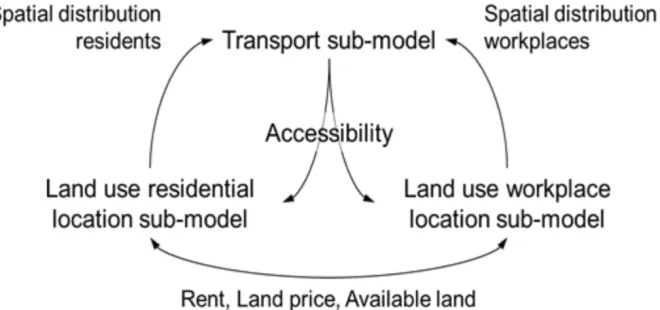
period. Figure 1 shows an overview of the MARS model. There are three sub-models within MARS, viz., transport, residential location and workplace location sub-models. The transport sub-model determines the demand for travel between zones for a given land use pattern and estimates the number of trips by a given mode of transport such as car, bus, train, walking and cycling for peak and off-peak periods. The output of the transport sub-model includes an accessibility measure which influences the residential and workplace location choices. Rents, land prices and land availability also influence where land is developed and the location choice of residents. These sub-models then interact over time and the system responds to exogenous inputs for growth in residents, jobs and car ownership and to any policy intruments simulated. As MARS is not the main subject of this paper readers are referred to Pfaffenbichler et al (2010) for a more detailed description.

Figure 1 Overview of MARS model

3. CASE STUDY

In order to investigate the competition between cities and the impacts of competition on optimal tolls and other indicators, we have developed a simple hypothetical case study based on an aggregated representation of an existing “spatially” complex model. This follows the discussion in Ghaffarzadegan et al (2011) who highlight the benefits of using small system dynamics models in addressing public policy issues. They found that small models are beneficial in conveying the essence of the feedback mechanism in a concise manner especially to decision makers. We therefore developed our small system dynamics model by aggregating to 2 zones from a previously validated 33 zone model of Leeds. We then formed anidentical copy of the two zone model i.e. the twin city also has identical population, jobs and geographical land area. We then allowed interactions between the twin cities to develop our hypothetical twin city 4-zone model (see Figure 2).

Figure 2: The twin city zones

The forecast population in the 2-zone model of Leeds was approximated against that of the full sized Leeds model with 33 zones. This full sized Leeds model in turn was calibrated/validated to UK TEMPRO forecasts (DfT, 2010) in terms of population, jobs and workers as described in Pfaffenbichler et al (2010). Table 1 compares the projected population in the inner and outer areas (zone 1 and 2 in the 2 zone model) of the 2-zone small model with the 33-zone full size model of Leeds. This shows a close agreement between the 2 zone model and the 33-zone model projections and thus the small model is taken as a reasonable approximation to the large 33-zone model. Furthermore, it is noted that both models exhibit higher growth in the outer zones i.e. urban sprawl continues in Leeds as forecast by TEMPRO. This along with similar mode shares between models give us confidence in our aggregate model for the purposes of this paper.

Table 1 Population of Leeds in Year 30

Region

2-zone model

33-zone model Zone1 (1-13 of 33 zones) 342879 343384 Zone2 (14-33 of 33 zones) 621780 621801 Total 964659 965185

In what follows, each city may decide to charge car users to travel to the central area (zone 1 in city A and zone 3 in city B) within the peak period. A charge will be equally applied to their own residents as well as the non-residents from the other city for crossing the cordon around the central zone in city A/city B.

3.1 Welfare measure

Local authorities of each city are assumed to maximise the welfare of their citizens. The traditional form of welfare within the transport field is the Marshallian measure which sums consumer and producer surplus. For tolling, the welfare measure includes the assumption that all revenues collected are recycled within the system by reinvesting to improve the transport system. For our case the measure may be estimated by the so called “rule of a half” (Williams, 1977) and so the particular welfare measures for each of city A and city B are written as below:

= + [ ( + )] [ ( + )] +

+ (1)

= + [ ( + )] [ ( + )] +

where,

= travel time between each Origin destination (OD) pairijwith road charge = travel time between each OD pairijwithout road charge

= trips between each OD pair with road charge = trips between each OD pair without road charge

, = toll charge to enter the central zone in city A or city B = Value of travel Time2

(VoT)

Equation (1) sums the rule of half time benefits and the rule of half money benefitswith the netrevenue collected by city A. The time and money benefits include the savings accrued to all trips originating from city A, i.e. i= 1,2, destined to any of the zones in city A or city B i.e. j = 1,2,3,4. This means time savings to residents of city A are accounted for across the two cities. However, the net revenue collected by city A is equal to the sum of the toll revenue from city A’s residents and that from city B’s residents and a transfer term is included to account for the toll paid to city B by the residents of city A. These revenue terms which transfer funds between the cities are important and form the basis of the tax exporting mechanism. An identical logic has been used to derive the welfare sum for city B as shown in equation (2).

It is noted that the welfare measure adopted in this research is a simplified version of the full scale of welfare. It is further simplified by considering the impact on private traffic in the peak hours only. However, we affirm that this is not too simplistic as it does account for the main impacts of a peak charging scheme, i.e. private traffic time savings and the monetary impacts of a peak charge whose revenue is assumed to be ear-marked for the city. Moreover it is also noted that the time savings to the private traffic also takes into account the effect of modal shift towards public transport as well as the re-distribution of trips. However, a full scale welfare function would also include the benefits accrued to public transport passengers and those using slow modes. As we are interested in peak road user charging only in our study then the monetary and time benefits accruing to the private car users would tend to dominate the full welfare function and so the welfare functions described in (1) and (2) are taken to be sufficiently robust to offer interesting insights into the dynamics of competition between the cities when considering only road tolls of this nature.

For a global regulator the welfare is simply equal to the sum of the welfare of city A and city B which is written as:

= +

(3) Note that in equation (3) when the welfares of city A and city B are summed together the non-resident toll revenue transfers between city A and city B cancel out with each other i.e. there is no benefit or consideration of tax exporting behaviour in the pareto or regulated case. In all cases below, the benefit streams generated over the 30 year study period will be discounted to form a Net Present Value (NPV) of benefits (discounted at 3.5%, DfT 2011). The notion of NPV is commonly followed in transport project appraisals where the revenue streams usually accrue from a long horizon period such as 25-30 years and it also helps in summarising the benefits (welfare) for making policy decisions.

2

3.2 Welfare profiles

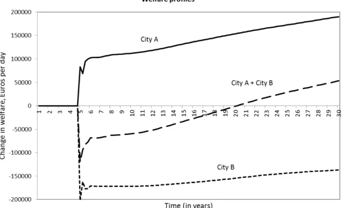
Before presenting the various scenarios below, it is useful to look at how the welfare measures evolve over time and how the individual and collective benefits vary when a toll is imposed. Figure 3 shows how the welfare varies over time for City A, City B and in total as city A charges a toll of 5€from year 5 onwards.

Figure 3 Variation in welfare over time when city A charges€5

From the figure we can see that when the charge is applied there are immediate positive benefits to city A which increase steadily over time as the demand from exogenous growth in population provides more potential for time savings compared to the do-nothing case. The benefits are made up from a combination of time and money benefits and a significant proportion comes from the revenues collected from city B’s residents. City B’s residents whilst benefitting from some time savings, lose all the toll revenues paid to city A and so the welfare change for City B is negative. The total welfare only becomes positive after year 20 when the time savings out-weigh the money losses in the system. Note that in the first year of implementation the benefits oscillate for a few months as the users take time to respond to the charges by changing behaviour until a new dynamic equilibrium is found. Whilst city A gains significantly from a charge of 5€, city B obviously loses out and given the symmetry of this case study we would expect them to react with a charge of their own. There is obviously an incentive to begin charging for both cities from the above figures assuming that the other does not also charge.

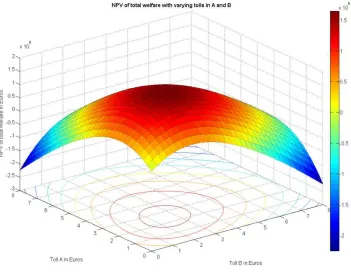
incentivised to toll. The Nash Equilibrium solution in this case will be where the derivative of own city welfare with respect to own toll is zero for both cities. Due to the symmetry in this case, we can plot the point of intersection between the line where the gradient equals zero and the equal toll line and so the Nash Equilibrium solution should be found for a toll of around 6€as shown by point N. Figure 4b shows the NPV of total welfare as tolls are varied. From this we may expect a global regulator to implement equal tolls of around 2.5€ to maximise total welfare.

Figure 4(b) NPV of total welfare

3.3 Modelled scenarios

This section sets out the two modelled scenarios as below:

 Regulated (Pareto) case

 Non co-operative game (Nash Equilibrium)

The first of the above is the regulated or pareto case where tolls are set by the regulator to maximise the total welfare of all residents as set out in (3). The second is the non-cooperative game (Nash Equilibrium) where cities aim to maximise their own residents’ welfare in a non-co-operative environment as set out by equations (1) and (2) for city A and city B respectively. This latter scenario turns out to be similar to the classic PD game. In this scenario, tax exporting behaviour is assumed and revenues arenotrecycledbetweenthe cities but recycled within the charging city. Note that for this symmetric case we only need to consider one city in presenting the results as the tolls will be identical.

3.4 Optimal tolls and welfare

In order to find the optimal toll levels, the VENSIM optimisation tool was used to maximise the appropriate welfare measure by varying the values of the relevant tolls. Note that to calculate the Nash Equilibrium solution, a diagonalisation approach was used whereby City A maximises their own welfare first with tolls for City B held constant, and then city B optimises their welfare with tolls for city A held at the previous iteration value. This was repeated until convergence, which was usually found to be within three to four iterations of each game.

Table 2 shows the optimal tolls and NPV of welfare change for each city per day plus the total welfare change for both cities for the symmetric cases.

Table 2: Tolls and NPV of welfare changes per day

Scenario

Optimal Tolls€

NPV of Welfare A€

NPV of Welfare B€

NPV of Total Welfare€ Regulated (Pareto) case 2.53 815,761 815,761 1,631,522 Non-cooperative game 6.08 -127,729 -127,729 -255,458

Table 2 exposes a number of observations. Note first of all that the optimal tolls found by the VENSIM optimisation facility for the Nash Equilibrium and the Regulated case are in line with the grid search shown in Figures 4(a) and 4(b). The welfare for city A is significantly higher when A tolls alone (Figure 4a) which reduces when city B also charges. This means that the increase in welfare of city A is at the expense of those residents in city B, but the total welfare change over both cities shows that together they are worse off as the total welfare change is negative as confirmed by the PD game shown in Table 2.

Due to symmetry, the tolls under the regulated or pareto case are equal and are the lowest tolls between the two scenarios. As expected, the pareto case returns the highest total welfare but the welfare to each city is much lower than could be achieved if only one city charges as can be inferred from figure 4a. The most interesting case is the non-cooperative game where both cities engage in a competition which then results in the highest tolls. In the end, both cities are worse off than in the no toll case with a significant reduction in welfare. They are not only worse off than the no toll case, but they are much worse off than if both had cooperated (as shown by the pareto case). This is the classic outcome of a PD game sometimes referred as a ‘Nash Trap’ which also appeared in the work of Koh et al (2012). Furthermore, we also note that there is no Local Nash Equilibrium (LNE) at any other toll levels as in Koh et al (2012). The LNE reported in Koh et al was due to the inclusion of route choice within the model and the specifics of their network. The fact that we have only one Nash Equilibrium solution simplifies the discussion around policy implications as there are no local solutions which lie close to theparetosolution as was the case elsewhere.

4. DYNAMIC GAME SET UP

five year plans and monitor and evaluate the impacts over time via a set of mandatory indicators, (DETR 2000).

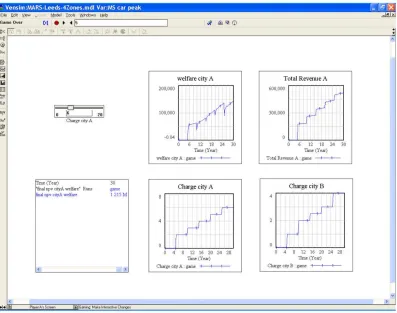
Figure 5 shows a screen shot of the view available to player A. The player sees his own charge which can be set every 5 years with the slider, the impact of both player’s charges on their own residents’ welfare measure, the total revenue collected in their city and the charges set in previous periods by the other player. At the end of the game they can also view the NPV of welfare change over the whole period in the table for their residents only (bottom left of the screen).

The game is played between two players each representing a given city. The two cities being identical in all respects including population, number of jobs, modes of transport available, it does not matter who is allocated to a given city. Each game is played over a period of 30-years stepping through 5-30-years each at a time and both the players make their decisions simultaneously on the amount of toll to set for the next five year period. The first five year period is taken as the warm up period and no tolls are needed to set, thus in a period of 30-years, players need to make five decisions each at year 5, year 10,…,year 25.

Each game is repeatedsix times meaning each player makes 30 (=5×6) decisions in all and thus between the two players 60 (=30×2) decisions will have been made. The game set up described here is similar to the repeated PD game described in the literature (e.g. Axelrod and Hamilton 1981) except that the decision on the amount to toll is in continuous terms whereas the standard PD game needs a binary decision (cooperate or defect). In our continuous PD game, the payoff matrix is also more complex to understand as the response surface (i.e. the welfare surface) depends on the response of the residents to the tolls. In addition the congestion benefits available from tolling increase over time as the population is increased. Whilst this is a complex game, it is designed to be realistic in that planners face exactly this type of problem when interpreting results from their (even more complex) models. Ideally our experiment would have involved real transport planners, however as we did not have access to enough planners we recruited players from masters and PhD students at the Institute for Transport Studies, Leeds who are exposed to the principles of transport policy and who may be considered to represent transport planners (at least they are expected to be a better representative sample than if recruits were drawn from the general public). The experiment conducted is described further in the next paragraph.

know the welfare of the other player until each round is completed i.e. when the time step reaches the 30 year mark. At the end of each round, the moderator announced the NPV of welfare and the final toll value for each city and both players were asked to record both sets of results in a table (See TableA.1 in Appendix A). The moderator then declared the player with the highest NPV of welfare as the winner for the round just finished and restarted the game for the next round until all six rounds were played.

Figure 5: Screenshot of player A’s screen

The entire gaming experiment was designed in such a way to test whether offering information about the benefits of collaboration or regulation would change the way in which the players behaved during the games. If the act of playing the game through the planning tool with information about the regulated solution can change behaviour, then this may have significant implications for the regulation of city strategies. We hypothesise that if they accept the regulated solution, then they avoid the Nash Trap and education about collaborative benefits is something which may be pursued rather than regulation.

5. RESULTS

This section presents an analysis of the gaming results. Firstly, it is useful to aggregate the results of the informed group into four sub-groups to analyse the impact of information received by the group members after game

Within each sub-group there are 8 players, 3 games and 5 decisions per game i.e. a total of 8×3×5=120 decisions per sub-group. In addition we are also able to compare with the control groupgames 1-3 and games 4-6 for each player A and B designated as below:

CtrlA1-3: control group player A games 1-3 CtrlA4-6: control group player A games 4-6 CtrlB1-3: control group player B games 1-3 CtrlB4-6: control group player B games 4-6

Before presenting an aggregate analysis of start charges, end charges and NPV of welfare we first discuss a typicalgame 3and typicalgame 6which represents behaviour before and after the regulator solution was shown to the players within the informed group.

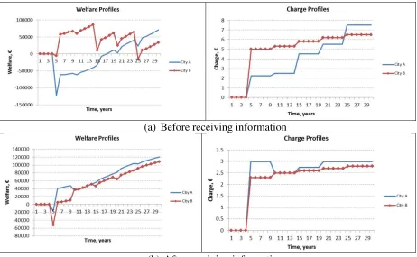
Figures 6a and 6b show the charges and welfare changes per day for both players for games 3 and 6 from a typical pair of players within the informed group.

(a) Before receiving information

(b) After receiving information

Figure 6(a), (b) Typical games before and after receiving information on optimal tolls

5.1 Mean value of charges before and after information

Table 3 shows the mean and variance of the charges at the start of the game and the end of the game period for each group. Taking the end values first, we can see that the mean values for both players A and B are reduced in games 4-6 after the regulator information compared with games 1-3. Paired t-tests show that these differences before and after information is given are statistically significant with p-values all below the Bonferonni adjusted critical value of 0.0083 (see Appendix B). The differences between players A and B for both sets of games were also shown to be insignificant so we can conclude that the players were acting in a similar manner whether assigned to A or B. It is noticeable that the mean values of 3.79 and 3.64 are still higher than the optimal flat toll of 2.53€. It should however be noted that other tests involving a linearly increasing toll over time showed the optimal toll to start at around 2€and increase to 3.0€, so some higher value may be expected.

Table 3: Mean and variance of toll charges Charge at the start Charge at the end Group Mean,€ Variance Mean,€ Variance

InfA1-3 3.99 6.75 6.29 15.47

InfB1-3 4.10 5.34 7.81 19.47

InfA4-6 2.88 1.27 3.79 2.93

InfB4-6 3.05 1.49 3.64 2.30

CtrlA4-6 7.46 19.7 7.76 27.6

CtrlB4-6 7.12 6.61 9.91 34.5

The start values show a slightly different pattern of results. Whilst the mean values for games 4-6 are reduced to 2.88 and 3.05€ for groups A and B respectively, these are not statistically different to the values from games 1-3. This is a reflection of the higher variance seen in the first three games where players are more prone to varying the starting point to assess the impacts of different charging regimes. The fact that the variance is reduced significantly in the subsequent games reflects the players’ newly developed knowledge of the outline of the welfare surface helped by the information just received. More significantly it represents the acceptance of the information and willingness to collaborate with a low toll solution. This fact is further confirmed by the comparison with the control group start and end charges for games 4-6 (CtrlA4-6, CtrlB4-6) in Table 3 where they are seen to be statistically lower than the control group charges (See Table B4, B5 in the appendix).

5.2 NPV of welfare results

This section compares the outcomes of the games in terms of NPV of welfare change for each city for each game and the mean values for the groups of games and players.

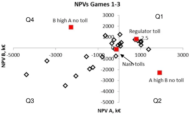
simulation experiments reported by Kunc and Morecroft (2010) we may split the space into the four quadrants as follows:

Quadrant 1: cautious movers. Both NPVs are positive. This comes about when tolls are relatively low and are bound by the optimal regulator solution;

Quadrant 2: NPV A positive, NPV B negative: player A generally plays a higher toll than B while B chooses a low toll. The benchmark solution is the A solo optimal toll;

Quadrant 3: aggressive movers. Both NPVs are negative. Both A and B play relatively high tolls which may result in highly negative outcomes for both players. Outcomes can be much worse than the Nash Equilibrium solution if both tolls are very high; and

Quadrant 4: the symmetrical opposite of Quadrant 2.

This split into quadrants is useful in describing the aggregate results across the 30 year period in each game and is similar to the 2*2 matrix often used in a PD game analysis, though in our case we distinguish co-operate and defect strategies indirectly via the final outcome or payoff. Q1 is where we see mutual co-operation, Q3 is where both defect and Q2 and Q4 are where one cooperates and one defects and one player receives the “sucker’s” payoff. The next section looks at the individual PD games at each decision point and hence individual strategies for the repeated game in more detail.

Figure 7: NPV results informed group games 1-3

Q1

Q2 Q3

Figure 8: NPV results informed group games 4-6.

Figure 9: NPV results for the control group games 4-6

From the figures we can see that in the first three games there are more solutions resulting in negative welfare for at least one player than there are solutions which result in positive welfare for both players. There are nine solutions where the welfare is highly negative for both players and the welfare losses are orders of magnitude worse than the Nash Equilibrium solution which shows that players can easily fall into a battle of the tolls.

In contrast after receiving information, Figure 8 shows that the outcomes are mainly located in Quadrant 1 where both players receive positive outcomes. Three of the solutions result in negative outcomes for player A which are a result of player B defecting to a higher toll rather than collaborating. However there are many more games where the players collaborate and do not defect to higher tolls. This suggests there is some benefit in the information given and that as it is possible to change tolls every five years, there is a threat of both players receiving significant losses if both defect to higher tolls which appears to maintain the collaboration. Figure 9 shows the same scatter plot of NPV for the control group games 4-6. The spread of results is similar to those from games 1-3 and contains only a few results within the first

Q1

Q2 Q3

Q4

Q1

Q2 Q3

quadrant. This suggests that the uninformed players are continuing with the aggressive or defection strategies more often than the informed players.

In addition to the figures discussed above, Table 4 shows the means and variances of the NPV of welfare values obtained in games 1-3 and games 4-6 for players A and B. As with the end charges, the mean values are not statistically different between players A and B but are statistically different between games 1-3 and games 4-6 (see Appendix B for p-values). The mean values are seen to change from negative changes in welfare to positive ones (although still lower than the value possible from the pareto case). In addition the variance between games is also reduced all of which suggests that the players have learned that collaboration is beneficial. Finally, the informed group NPV of welfare for games 4-6 is also statistically different to that of the control group values shown in Table 4 (see Table B6 of Appendix B for p-values).

Table 4: Mean and variance of NPV of welfare Net Present Value of

welfare per day

Group Mean,€ Variance InfA1-3 -533,015 2.10E+12 InfB1-3 -344,356 1.64E+12 InfA4-6 599,235 2.10E+11 InfB4-6 632,732 1.78E+11 CtrlA4-6 -1,817,059 9.64E+12 CtrlB4-6 -1,586,921 7.93E+12

5.3 Analysis of gaming strategies

In a standard repeated PD game, it is standard practice to analyse the strategies of players in terms of whether players repeatedly co-operate or defect and one can even look for evidence of tit for tat and end game defections as described in section 1. Despite our game being a continuous or extensive form game with the added complications that (a) the players do not know the response surface or payoff in advance and (b) that while the game is repeated 5 times within a round, each game is connected to the previous decision and the response surface or payoff changes gradually with a growth in the population; we are still able to analyse the level of co-operation and defection.

Table 5 : The definition of co-operation and defection using welfare gain in each period Player B

Player A

Cooperation Defection

Cooperation Both players receive a positive gain in local welfare in period

Player A negative welfare gain in period

Player B positive welfare gain in period

Defection Player A positive welfare gain in period

Player B negative welfare gain in period

Both players receive a negative welfare gain in period

This definition follows the standard PD game approach, and is set in terms of the outcome rather than the input strategies (tolls in our case). It should be noted that while in a discrete game the strategies are limited and usually obvious in terms of whether they are co-operative or not, in our case a toll of say 4€ may be deemed as co-operative or as defection depending on the level played by the opposing player. It can be inferred from the response surface in Figures 4a,b that where both players toll 4€ then both receive a positive welfare gain; however if one player were to toll only 1€ then that player would receive a negative welfare gain or a loss in that period. In this case the player which plays the higher toll receives a higher welfare gain and is said to be the “defector” while the low toll player receives the “sucker’s payoff as defined by Axelrod and Hamilton (1981). In reality, some of the combinations recorded in our experiment will be “more” co-operative than others (where both players receive a highly positive welfare gain), some will lie on the boundary of the region where both players receive a positive welfare gain (just inside the defection boundary) and others will give extremely negative outcomes for both players. The table is a simplification of the true response surface and is related to the quadrants investigated earlier under the NPV analysis which looked at the outcome over the whole game.

5.3.1 Evidence of reciprocity and cooperation

Given the definition above, table 6 shows the number of decisions which were mutually cooperative, mutually defective and with one defective and one cooperative player for each group of games for both the informed and control groups.

Table 6: Cooperation or defection? Proportion of decisions by group Group/games Both players are

cooperating (CC)

Both players are defecting (DD) One player cooperates and one defects (CD/DC) Informed games 1-3

49 (41%) 40 (33%) 31 (26%)

Informed games 4-6

101 (84%) 4 (3%) 15 (13%)

Control games 1-3

35 (29%) 48 (40%) 37 (31%)

Control games 4-6

Firstly, table 6 shows that there is no difference in the strategies played by the control group between games 1-3 and 4-6 with cooperation levels consistently at 28 or 29%. This level of cooperation is not unexpected as it has been seen in previous repeated game experiments where partners may build a level of trust. However the overall strategy is that of defection with around 50% of decisions being with both defecting and an additional 34-37% where at least one player defects. The first three games for the informed group display slightly higher levels of cooperation with 41% but this is still way below that seen in the literature e.g. in Andreoni and Miller (1993) where partners were found to cooperate more than strangers with levels as high as 50% even in the later rounds. The effect of information prior to games 4-6 has a significant effect on the level of cooperation with 84% of decisions being mutually cooperative and the level of double defection dropping from 33% to only 3%. There still exists some level of defection (13%) where one player changes strategy and this is also expected especially towards the end of the period as an end game effect.

The strategies played by each pair of players for each round and game is shown in tables C1 and C2 in Appendix C using “CC”, “DD”, “CD and “DC” to denote both co-operate, both defect, A co-operates and B defects; and A defects and B cooperates. Using this notation it is possible to visualise the strategies. In general for the uninformed games (control group and games 1-3 of the informed group) the strategies are characterised by defection of both or one player. Pair 5 (informed) and pair 7 (control) show a high degree of cooperation in all games and this could be a result of initial exploratory strategies resulting in both receiving positive outcomes – they stumbled across the cooperative game and chose to sustain it. Again this is not unexpected as previous literature has shown that a proportion of the population are altruistic in their responses.

From the informed games (4-6 informed group) it can be seen that after receiving information about the regulated solution the players adopt a tit-for-tat co-operative strategy in most instances and that this cooperation is sustained (see for example pairs 1,3,5,6,7,8). There is no real evidence of an end game tactic where one player suddenly defects as has been seen in previous experiments. This may be due to the relatively low number of games played after receipt of information. Only pair 8 displayed an end game effect in game 5 round 5. Other pairs co-operated in the majority of rounds after receiving information though there was some attempt to defect in early rounds – e.g. pair 4. Here player B tolled 4€ initially while player A tolled 2€and in subsequent rounds player B waited for player A to catch up in terms of toll level and so cooperation evolved.

5.4 Implications for transport policy

The results of this research may have significant implications for transport policy followed by local authorities:

 Firstly, the results clearly showed that there is an incentive to cooperate at local authority level rather than compete with each other. Whilst not related to toll competition per se, this move towards more collaboration between authorities has been reflected in the move towards regional planning and the creation of the city regions in England. In fact at the time of writing, the West Yorkshire authorities were combined with York and transport planning is now overseen by the newly formed Integrated Transport Body.

information is encouraging in that it implies information rather than regulation may be used to influence and improve transport polices. However, this result should be treated with some caution as we have only investigated a two player game here and as discussed earlier Dawes (1980) has pointed out that such cooperation may not be sustained where there are more than two players involved. Despite this, it is encouraging that the Integrated Transport Body for the Leeds region (LCR, 2013) (which includes ten local authorities) is forming strategies based on collaborative outcomes informed by a regional model.

 Thirdly, it is noted that although the cities modelled in this experiment are taken to be identical, the analysis has provided insights in understanding the dynamics between the players. However, in real life, cities are less likely to be identical and one city may exert greater power over its neighbour. We have tackled this issue in another paper (Shepherd and Balijepalli 2012b) and found that regulation would be required as there would be less incentive for the more powerful city to accept the co-operative solution.

 Finally, while the devolution of powers to city regions helps in providing a forum for collaboration at the regional level and while this may prove useful in promoting collaborative schemes, it does open up the opportunity for competition at the regional level e.g. between the Leeds City region and the Manchester region where regions now compete for capital growth funding and other more strategic investments. In these cases, the rewards (for defection) are likely to be greater and the possibilities for mutually co-operative outcomes lower. This type of competitive environment is obviously a key area for further research of this kind.

6. CONCLUDING REMARKS

In this paper we first of all applied the MARS Land Use Transport Interaction Model as a planning tool to demonstrate the potential optimal tolls for two neighbouring cities. Used in this way we showed that for a one-shot game where cities set a toll for the future and stick to that toll then a Nash Trap exists which would result in negative welfare changes for both cities. We also showed that both cities would benefit from a lower toll regime under some form of regulation. These results were in line with the earlier research conducted with a static network assignment model as reported in Koh et al (2012). We then applied the simulator in a game playing mode to test how decision-makers would update their strategies in response to cues including charges set by the other city and changes in own city welfare over the previous periods.

For theinformed group, the game was repeated three times before information about the low toll regulator solution was presented to the participants and the game repeated a further three times. The mean values of the end charges for the games 4-6 were seen to be statistically lower than those in games 1-3 and those in games 4-6 from the control group. The NPV of welfare changes were also statistically higher and now positive in games 4-6 and were statistically different to the values from the control group.

While the control group players behaved consistently through the six games, the informed group players’ level of cooperation more than doubled after receiving the critical information on optimal tolls and welfare. Similarly the rate of both players defecting fell sharply in games 4-6 of the informed group.

to come about naturally and has been observed in both the economics (Bolton and Ockenfels, 2000) and the game theory literature, Dufwenberg and Kirchsteiger (2004), Falk and Fischbacher (2006). The levels of cooperation after information we around 84% which is very close to the 86% level found by Andreoni and Miller (1993) in round 1 of their games where partners were able to build trust. This behaviour is important as it suggests that by providing information about the regulated solution where both parties receive welfare improvements, that players will respond positively and that a Nash Trap may be avoided. This result brings into focus the question of how cities actually make decisions about future strategy. If they plan using models of the future and apply one shot strategies then they may find themselves in a Nash Trap with higher tolls imposed on the general public. If however they make decisions and regularly review them against a set of indicators and benchmark against others’ actions then improving information about the benefits of collaboration may result in lower tolls and welfare improvements.

We suggest that education through gaming or simulators such as MARS rather than direct regulation may be used in developing transport strategies across regions or where there are more than one interested party involved. This education over regulation will though only be plausible in cases where there exists the opportunity to demonstrate reciprocal behaviour over a period of time or where it is obvious that defection may be punished in subsequent periods. These results could have significant implications for the development of city strategies within regional partnerships, something which will become more common with the current government’s devolution of power and the establishment of local transport bodies to oversee spending on major schemes from 2015. Future research is needed to include not only the objectives of local authorities within the model but also objectives and responses of other stakeholders such as local transport operators.

Acknowledgement: We thank the UK Engineering and Physical Science Research Council (EPSRC) for funding this research via grant EP/H021345/01. We also thank the two anonymous referees for their helpful comments in improving the quality of the paper. An earlier version of the paper (Shepherd and Balijepalli 2014) was presented at the 32nd International Conference of the System Dynamics Society held at Delft, Netherlands, 20-24 July 2014.

References

Andreoni, J., and Miller, J.H. (1993). Rational cooperation in the finitely repeated prisoner’s dilemma : experimental evidence. The Economic Journal, 103 (May) 570-585.

Anas A & Pines D (2008) Anti-sprawl policies in a system of congested cities. Regional Science & Urban Economics38, 408-423.

Axelrod, R. and Hamilton, W.D. (1981). The evolution of cooperation. Science, New Series, Vol.211 (No.4489), 1390-1396.

Basolo V (2000) City spending on economic development versus affordable housing: Does inter-city competition or local politics drive decisions? Journal of Urban Affairs41(3), 683-696.

Brueckner JK & Saavedea LA (2001) Do local governments engage in strategic property-tax competition? National Tax Journal54(2), 203-229.

Cooper, R. et al (1996). Cooperation without reputation : experimental evidence from Prisoner’s dilemma games. Games and Economic Behaviour 12, 187-218. Article No.13.

Dawes, R.M. (1980). Social Dilemmas. Annual Reviews. Psychology. 1980. 31:169-93 DCLG & DPMO (Department for Communities and Local Government & Deputy Prime

Ministers Office) (2012) https://www.gov.uk/government/publications/city-deals-wave-1, web site accessed on 27 January 2014

De Borger B, Dunkerly F & Proost S (2007). Strategic investment and pricing decisions in a congested transport corridor. Journal of Urban Economics62, 294-316.

De Palma A, Lindsey R (2000). Private Roads: competition under various ownership regimes. Ann of Reg Sci34, 13-35

DETR (Department of Environment, Transport and the Regions) (2000) Guidance on Local Transport Plans. DETR, London, UK.

DfT (Department for Transport) (2010)http://www.dft.gov.uk/tempro/web site accessed 8 March 2012.

DfT (2011)http://www.dft.gov.uk/webtag/documents/project-manager/unit2.7.1.php. Web site accessed 19 July 2013

Dufwenberg, M. and Kirchsteiger, G. (2004) A theory of sequential reciprocity. Games and Economic Behaviour 47 (2004) 268–298.

Falk, A. and Fischbacher, U. (2006) A theory of reciprocity. Games and Economic Behaviour 54 (2006) 293–315.

Ghaffarzadegan, N., Lyneis, J. and Richardson, G.P. (2011) How small system dynamics models can help the public policy process,System Dynamic Review27(1), 22-44. Haken, H. (1983). Advanced Synergetics - Instability Hierarchies of Self-Organizing Systems

and Devices, Springer-Verlag

Ho HW, Wong SC, Yang H & Loo BPY (2005) Cordon-based congestion pricing in a continuum traffic equilibrium system. Transportation Research39A, 813-834.

Ho HW & Wong SC (2007). Housing allocation in a continuum transportation system. Transportmetrica3(1), 21-39.

Holt, C.A. (1999) Teaching economics with classroom experiments. Southern Economic Journal, January 1999, 65(3), 603-610.

Koh, A., S.Shepherd and D.Watling (2012) Competition between Two Cities using Cordon Tolls: An Exploration of Response Surfaces and Possibilities for Collusion,

Transportmetrica(March 2012)DOI:10.1080/18128602.2012.673033

Kreps, D., Milgrom, P., Roberts, J. and Wilson, R. (1982). Rational cooperation in the finitely repeated prisoner’s dilemma. Journal of Economic Theory, 17, 245-252. Kunc, M.H., and Morecroft, J.D.W. (2010) Managerial decision making and firm

performance under a resource-based paradigm. Strategic Management Journal, 31: 1164–1182 (2010).

Levinson D and Yerra B (2006). Self Organization of Surface Transportation Networks. Transportation Science40(2) 179-188.

LCR (Leeds City Region) (2013)http://www.leedscityregion.gov.uk/about/web site accessed on 22ndJanuary 2014

Marsden, G. (2009) Congestion Pricing: Do We Need a New Approach to Parking Policy? Lessons from Europe, Presentation to 88th US Transportation Research Board Meeting, Washington D.C., January

Mun S, Konishi K & Kazuhiro Y (2005). Optimal cordon pricing in a non-monocentric city. Transportation Research Part39A, 723-736.

Pfaffenbichler, P., Emberger, G. and Shepherd, S.P. (2010): A system dynamics approach to land use transport interaction modelling: the strategic model MARS and its application.System Dynamics Reviewvol 26, No 3 (July–September 2010): 262–282. Roth, A.E. (1988) Laboratory experimentation in economics: a methodological overview, The

Economic Journal, Vol 98, No.393, (Dec 1988), 974-1031.

Shepherd, S. and Balijepalli, N.C. (2012a) A dynamic model of two competing cities: the effects of competition on tolls and land use. In the proceedings of the 30th International Conference of the System Dynamics Society, St Gallen, Switzerland, 22-26 July 2012.

Shepherd, S. and Balijepalli, N.C. (2012b) Symmetric and Asymmetric Interactions Between Competing Cities: The Long Term Response, In Proceedings of the 17th International Conference of the Hong Kong Society for Transportation Studies (HKSTS), 17-20 December, Hong Kong

Shepherd, S. and Balijepalli, C. (2014) A game of two cities: a toll setting game with experimental results. In the proceedings of the 32nd International Conference of the System Dynamics Society, Delft, Netherlands, 20-24 July 2014.

Shepherd, S.P. and Sumalee A. (2004). “A genetic based algorithm based approach to optimal toll level and location problems”.Networks and Spatial Economics,4.

Shepherd SP, May AD & Koh A (2008). How to design effective road pricing cordons. Proceedings of the Institution of Civil Engineers, Transport: Road User Charging,161, TR3, 155-165.

Sterman, J. (2000). Business dynamics : systems thinking and modelling for a complex world, Irwin/McGraw-Hill, Boston.

Sterman, J. (2014). Interactive web-based simulations for strategy and sustainability : The MIT Sloan LeraningEdge management flight simulators, Part I. System Dynamics Review. Volume 30, No1-2 (January-June 2014) : 89-121.

Sumalee, A., May, A.D. and Shepherd, S.P. (2005). Comparison of judgmental and optimal road pricing cordons. Transport Policy, Volume 12, Issue 5 September 2005, pp384-390.

Tiebout CM (1956). A Pure Theory of Local Expenditures. Journal of Political Economy 64(5), 416-424.

Ubbels, B., Verhoef, E. T., (2008),“Governmental competition in road charging and capacity choice”,Regional Science and Urban Economics, 38(2), 174-190.

Verhoef E.T., Nijkamp P and Rietveld P (1996). Second-best congestion pricing: the case of an untolled alternative. Journal of Urban Economics40, 279-302.

Walters A (1961). Theory & Measurement of private & social cost of highway congestion. Econometrica29(4),676-699.

Williams, H.C.W.L. (1977) On the formation of travel demand models and economic evaluation measures of user benefit. Environment and Planning A, 1977, volume 9, pages 285-344.

Wilson, J.D. (1999) Theories of tax competition,National Tax Journal,52(2), 269-304 Yang H. Xiao F., Huang H., (2009) “Private Road Competition and Equilibrium with Traffic

Equilibrium Constraints”Journal of Advanced Transportation, 43(1), 21-45.

Appendix A: gaming brief

Competition between cities: a game to maximise welfare with road user charging

(for the group with information given after 3 rounds)

Consider two identical cities located near to each other. Both are planning to introduce cordon-based road user charging to enter the inner city area (zones 1 or 3 above). You will act as the local authority for one of the two cities and your aim is to maximise the welfare to your city and its residents by setting a toll around your cordon. You will need to decide the toll amount after every 5 years. Note that the toll to enter your city is applied to both your residents and the residents from the other city who wish to travel to your inner city area and that all the revenue collected will be retained by your city.

Each game will be played for a period of 30 years and the city withhighest welfare(the net present value of)wins the game. The first five year period is considered as a warm up period during which period no tolls are collected.

After every 5 year period you will be able to see the profiles of your city’s welfare, total revenue collected by your city, charge applied in your city and the charge set in the other city. At the end of each game you will also see the Net Present Value of the change in welfare for your city and the moderator will announce the Net Present Value for both players.

You will havesix rounds of the game. After each round you are required to record the final year charges and the net present value of welfare in year 30 for both players in a blank table supplied to you overleaf (Table A.1)

After three rounds into the game, you will be given information on optimal tolls which may be found useful in the subsequent rounds. (This sentence has been deleted for the controlled group experiment)

Note:You are not allowed to communicate your strategies to the other player during the game.

Table A.1 Competition between cities: a game to maximise welfare with road user charging

Record of final year charge and NPV of welfare

Round # Final Year Charge,€ NPV of Welfare,€

City A City B City A City B

1

2

3

4

5

Appendix B: Statistical inference of gaming results

Table B1: t-test: p-values for paired charge values at start

Group A1-3 B1-3 A4-6 B4-6

A1-3 - 0.8817 0.0647 0.1184

B1-3 - 0.0271 0.0579

A4-6 - 0.6243

B4-6

-Table B2: t-test: p-values for paired charge values at end

Group A1-3 B1-3 A4-6 B4-6

A1-3 - 0.2158 0.0076 0.0044

B1-3 - 0.0003 0.0002

A4-6 - 0.7453

B4-6

-Table B3: t-test: p-values for paired NPV values

Group A1-3 B1-3 A4-6 B4-6

A1-3 - 0.6353 0.0011 0.0008

B1-3 - 0.0020 0.0014

A4-6 - 0.7933

B4-6

-Table B4: t-test: p-values for paired charge values at start

Group A4-6 B4-6

ConA4-6 0.002367 0.003896 ConB4-6 0.001464 0.002084

Table B5: t-test: p-values for paired charge values at end

Group A4-6 B4-6

ConA4-6 0.001504 0.000998 ConB4-6 0.000225 0.000156

Table B6: t-test: p-values for paired NPV of welfare values

Group A4-6 B4-6

Appendix C: Strategies played by individuals

Table C1 : Strategies played by informed group

Pair Round

1 Game 1 2 3 4 5

1 DC CC CD CD CD

2 DD DD DD DD DD

3 CC CC CC CC CC

4 CC CC CC CC CC

5 CC CC CC CC CC

6 CC CC CC CC CC

Pair Round

2 Game 1 2 3 4 5

1 DD DD DD DD DD

2 CD CD CD CD CD

3 DD DD DD DD CD

4 CD CD CD CD CD

5 DD DD DD CC CC

6 DC DC CC CC CC

Pair Round

3 Game 1 2 3 4 5

1 DC CD DD DD DD

2 DC DD DD DD DD

3 CD CD CC CC CC

4 CC CC CC CC CC

5 CC CC CC CC CC

6 CC CC CC CC CC

Pair Round

4 Game 1 2 3 4 5

1 DC DC DC DC CC

2 CC CC CC CC CC

3 CC CC CC CC CC

4 CD CC CC CC CC

5 CD CD CC CC CC

6 CD DC DD CC CC

Pair Round

5 Game 1 2 3 4 5

1 DC CC CC CC CC

2 CC CC CC CC CC

3 DC CC CC CC CC

4 CC CC CC CC CC

5 CC CC CC CC CC

6 CC CC CC CC CC

Pair Round

6 Game 1 2 3 4 5

1 CD CD CC CC CC

3 DD DC DD DC CC

4 CD CC CC CC CC

5 CC CC CC CC CC

6 CC CC CC CC CC

Pair Round

7 Game 1 2 3 4 5

1 CD CC CC CC CC

2 DD DD CC CC CC

3 CD CD CC CC CC

4 CC CC CC CC CC

5 CC CC CC CC CC

6 CC CC CC CC CC

Pair Round

8 Game 1 2 3 4 5

1 DD DD DD DD DD

2 CD DD DD DD CD

3 DD DD DD DD DD

4 CC CC CC CC CC

5 DC CC CC CC DC

6 CC CC CC CC CC

Table C2 : Strategies played by control group

Pair Round

1 Game 1 2 3 4 5

1 DD CC CD CC CC

2 DD DD CD CC CC

3 CC CC CC CC CC

4 DC DC CC CC CC

5 DC CC CC CC CC

6 CC CC CC CC CC

Pair Round

2 Game 1 2 3 4 5

1 DD DD DD DC DC

2 DD DD DD DC DC

3 DD DD DD DD DC

4 DC DC DC DC CC

5 DC DC DC DC CC

6 DD DD DC CC CC

Pair Round

3 Game 1 2 3 4 5

1 DC DC DC CC CC

2 CD DD CD CD DD

3 DD DD DD DD DD

4 DD DD DD DD CD

5 DD DD DD DD DD

6 DD DD DD DD DD

4 Game 1 2 3 4 5

1 CD CC CC CC CC

2 DD DD DC DC CC

3 DD DD DD DD DD

4 DD DD DD DD DD

5 DD DD DD DD DD

6 DD DD DD DD DD

Pair Round

5 Game 1 2 3 4 5

1 CC CC CC DC DC

2 DC CD CD CD CC

3 CD DD DD DD DD

4 CD CD CD DC DC

5 DD CD DD DD DD

6 CD DD DD DD DD

Pair Round

6 Game 1 2 3 4 5

1 DC DC DC DC DC

2 DC DD DC DC DC

3 DD DD DD DD DD

4 DD DD DD DD CD

5 CD CC DD CD CD

6 DD DD DD DD DD

Pair Round

7 Game 1 2 3 4 5

1 DC DD CC CC CC

2 DC CC CC CC CC

3 CC CC CC CC CC

4 DC CC CC CC CC

5 CC CC CC CC CC

6 DC CC CC CC CC

Pair Round

8 Game 1 2 3 4 5

1 CD CD CD CD CC

2 DD DD DD DD DD

3 DD DD DD DD DD

4 DD CD CC CC CC

5 CD DD CC DC CC