Estimating the Age of the Common Ancestor of a DNA Sample Using the Number of Segregating Sites

(1)

Copyright 0 1996 by the Genetics Society of America

Estimating the Age

of

the

Common

Ancestor

of

a

DNA

Sample Using

the Number

of

Segregating Sites

Human Genetics Center, University of Texas, Houston, Texas 770?0 Manuscript received March 8, 1996

Accepted for publication July 12, 1996

ABSTRACT

The number of segregating sites in a sample of DNA sequences and the age of the most recent common ancestor (MRCA) of the sequences in the sample are positively correlated. The value of the former can be used to estimate the value of the latter. Using the coalescent approach, we derive in this paper the joint probability distribution of the number of segregating sites and the age of the MRCA of a sample under the neutral Wright-Fisher model. From this distribution, we are able to compute the likelihood function of the number of segregating sites and the posterior probability of the age of the MRCA of a sample. Three point estimators and one interval estimator of the age of the MRCA are developed; their relationships and properties are investigated. The estimation of the age of the MRCA of human Y chromosomes from a sample of no variation is discussed.

T

HERE are considerable interests in the age of the most recent common ancestor (MRCA) of a DNA sample when studying the evolutionary history of a population from which the sample is taken. The current controversy on the age of the MRCA of modern humans attests the need of proper statistical methods for the inferences on common ancestry. Because an inference on the age of the MRCA has to be based on population samples, appropriate population genetics theory should be taken into account. The coalescent theory ( KINGMAN

1982a,b;

HUDSON

1983; TAJIMA 1983) is a natural choice because it deals with how the sequences in a sample coalesce to their common ancestors. In this paper, we shall present a coalescent theory that is neces- sary for the estimation of the age of the MRCA of a sample using the number of segregating sites and inves- tigate the properties of newly developed estimators from this theory.

The number of segregating sites in a sample of DNA sequences from a population is the simplest quantity observable. Since WAITERSON’S (1975) work, the number of segregating sites has been widely used for estimating the essential population parameter

0

= 4Np, where Nis the effective population size and p is the mutation rate per sequence per generation, and recently has been used for testing evolutionary hypotheses (e.g., TA-

JIMA 1989; FU and LI 1993b; Fu 1996). Although samples of DNA sequences have been used by several au- thors to estimate the age of human mitochondria, the sample by DORIT et al. (1995), which consists of 38 sequences from the intron of ZFYgene in the human Y chromosome, presented a special challenge because

Address fw correspondence: Human Genetics Center, University of Texas at Houston, 6901 Bertner Ave., S222, Houston, TX 77030. E-mail: [email protected]

Genetics 144: 829-838 (October, 1996)

there is no variation in this sample. Any estimator of the age of the MRCA that is proportional to the number of segregating sites or the mean number of nucleotide differences between two sequences will yield zero as the estimate, which is apparently unacceptable. DORIT et al. ( 1995) attempted to estimate the age of the MRCA of the human males from this sample, but their analysis was not rigorous ( FU and LI 1996; DONNELLY et aZ. 1996; WEISS and VON HAESELER 1996). FU and LI (1996) developed a method from the coalescent theory to deal with samples with no variation and reanalyzed DORIT et

aZ.’s sample. Their theory is extended in this paper to cope with samples with any number of segregating sites.

THE THEORY

We assume that the population under study evolves according to the Wright-Fisher model, that mutations in the locus from which DNA sequences are obtained are selectively neutral, that the effective population size is constant over time and that there is no recombination within the locus. We shall present our results for a sample of DNA sequences from an autosomal locus so

that the parameter

8

is defined as 4Np, where N is the effective population size and p is the mutation rate per sequence per generation. Our results also apply to a DNA sample from a mitochondrial locus by defining 0 as 2Nfp, where N, is the effective size of the female population, and to a DNA sample from a locus in Y chromosome by defining 8 as 2N+, where N,,, is the effective size of the male population.

The genealogy of a sample of n DNA sequences can be divided into n - 1 states numbered from 2 to n. State k is the period in which the genealogy has exactly

(2)

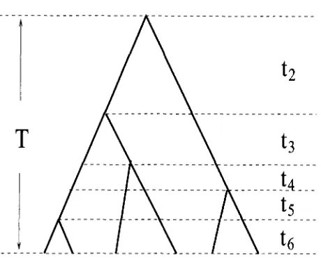
FIGURE 1.-An example of the genealogy of a sample of six sequences. T =

+

-

*

+

and the total time length

of the genealogy is L = 2t2

+

*

+

6 k . Dashed lines divide

T into five periods (states).

coalescent time. When sample is random, tk follows ap- proximately an exponential distribution with parameter

k ( k - 1 ) / ( 4 N ) (KINGMAN 1982b). The age ( T ) of

the MRCA of the sample is equal to

T =

,%+

+

t,

and the time length in the entire genealogy is L = 2,%

1 ) branches. Assume that the number of mutations in branch i conditional on the length 1, of the branch follows Poisson distribution with parameter lip. Then the number K of mutations in the entire genealogy conditional on the coalescent times t k ( k = 2 ,

. . .

,

n )

is the sum of 2 ( n - 1 ) Poisson variables and thus follows the Poisson distribution:

+

. . . +

nt,. The sample genealogy consists of

2

( n -

When the infinite-sites model is assumed, K is the number of segregating sites in the sample. Since different coalescent times are independent, the joint probability density of

,%,

. . .

, t, is thus

The joint probability that there are K segregating sites in the sample and that the k t h coalescent time ( k = 2,

. . .

, n ) is equal to t k is the product of ( 1 ) and ( 2 ) ,

namely

k ( k - 1) k ( k - 1 )

K ! exp[ - 4N t k ]

.

If coalescent times are rescaled such that one unit corresponds to 4Ngenerations, the above equation becomes

Throughout this paper, all times are so scaled when their units are not specified. Note that one unit of the scaled time will correspond to 2Nf generations if the locus is in mitochondria and 2Nm generations if the locus is in the nonrecombining region of Y chromosome.

It follows from ( 3 ) that the probability of the event that there are K segregating sites and that the age of the MRCA of the sample is Tis

k

This joint probability is the foundation for the inferences on T from K . We can show ( APPENDIX ) that

where

and

It is clear that there is only one term in the summation of Y K - I , k for 1 =

K ,

while the number of terms for

<

Kcan be shown to be

**CE=i;(K-L*n-2)**

(E;”’)

( y - ‘ ) ,

which is in the order of nK-‘. Therefore, it is not convenient to compute a k l directly from ( 6 ) when K

-

1 and n

are not small. Letting ( Y k l = a k l ( 2 ) , it can be shown (APPENDIX ) that ck!kl( 2 ) can be computed from the fol-

lowing iteration procedure:

k = i + 1, . . . , n

n

a i l ( i ) = - a k l ( i ) ( 9 )

k = z + l

for 1 = 0,

. . .

, K . The initial values for the iteration are

a,K(n) = 1, ana( n ) =

-

* = (YnK-, ( n ) = 0 . (10)

Two marginal distributions

p ,

( K ) and +n ( T ) can be

(3)

Estimating the Age of MRCA 831

of K and the latter the distribution of T. It is simple to show that

where

n K 11

Equation ( 1 1 ) provides an alternative way to compute the probability of K than the formula derived by TAVARE

( 1 9 8 4 ) . ( T ) can be obtained by summing

p,

( K , T ) over all possible values of K. Because # n ( T ) is independent of the mutation rate p, by setting p = 0 (thus

B

= 0 ) we have from ( 5 ) that # , ( T ) = n ! ( n - l ) !

x c

( - 1 ) k ( 2 k - l ) k ( k - l ) e - k ( k - l ) T k = 2 ( n - k ) ! ( n

+

k - l ) !

n

= ( - l ) k ( 2 k - 1 )

k = 2

This equation is equivalent to TAJIMA'S ( 1 9 8 9 ) Equa- tion 3, except that different time scales are used and that TAJIMA ( 1990) considered only the case n = 2N.

Incidentally, since the exponential distribution of a coalescent time is derived under the assumption that n 2N, Equation 13 should be applicable only to samples of sizes that are much smaller than 2N. Nevertheless, TAJIMA ( 1990) showed that

42N(

T ) is close to KIMURA'S

( 1 9 7 0 ) distribution of fixation time of a new neutral

mutant.

From the joint probability density

p,

( K , T ) and the

two marginal probabilities

p,

( K ) and

4n

( T )

,

two quan- tities that are essential for the inferences on T can be computed. One is the likelihood function

pn(

KI T ) of T and the other is the posterior probability

pn

( TI K )

of T , defined respectively as

The posterior probability is equal to n K

pn

( TI K ) = c i l

z

aklklT1e-k(e+k-l) ( 16)

k = 2 1=0

from which one can derive the conditional expectation and variance of T . It is a simple matter to show that

- E 2 ( T I K ) . ( 1 8 )

We now consider several situations in which Equation

5 is convenient to use directly. The first case is when K = 0. It is easy to see from ( 8 ) that Y O , k = 1 . Therefore

( Y k L = P k ( 8 ) , which implies that

n

p,(O, T ) = n ! ( n - l ) ! P k ( 8 ) e - k ( 8 + k - 1 ) T

.

( 1 9 ) k = 2

Since WATTERSON ( 1 9 7 5 ) showed that

n- I k 8 + k

P , ( K = 0 ) =

n

- _{( 2 0 )}

k= 1

the posterior probability

p,

( TI 0 ) becomes

P7l(

TIO)

L k = l k = 2

which was derived first by FU and LI ( 1 9 9 6 ) . Substitut- ing

P k

for akl in ( 1 7 ) and ( 1 8 ) we have

The likelihood function of Tis given by

The second situation is when K = 1 . We have from

( 8 ) that

n

1 _- 1

Y l , k % + k + i - l r=2 e + 2 k - 1 '

It follows that

n

p n ( 1 , T ) = 8 n ! ( n - I ) !

@ , ( e )

k = 2

1

x e + k + i - l

7 1

(4)

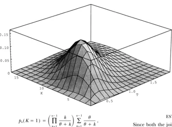
FIGURE 2."Surface of

p,,(

K , T )

when n = 30 and B = 2.0.

one can thus compute the values of the likelihood function and the posterior probability without using the iteration procedure specified by ( 9 ) and ( 10).

Finally since

>I

1 1

-

y 2 . k = C ( e + h + i - l ) ~ i=2 ( 8 + 2 k - 1 ) '

2 s i < j s n : i . j t k

(e

+

k + i -

l)(O

+

k + j -

1 ) '

which is also easy to compute, we have

,I

fi,l(29 T ) = 0 2 ? l ! ( n - I ) !

P k ( e )

k=2

X [Y2(kT)'+ Yl+k(kT)

+

y ~ ~ k ] e " " k - l ) " ' * (26)

Before we consider how to estimate T from the value of K, it is helpful to gain some ideas on the shape of the joint probability density fin ( K , T ) , the likelihood

function fin( KI T) and the posterior probability

f i l l ( TI K)

.

Figure 2 shows the surface of f i l l ( K, T ) for

a sample of 30 sequences and

I9

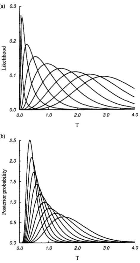
= 2.0.

It can be seen from Figure 2 that the peak of Tshifts with K and vice versa. Figure 3, a and b, shows the likelihood function and the posterior probability of T respectively, for a number of values of K. It is clear by comparing the two panels ( a and b ) that the value of

T corresponding to the peak of a likelihood function is smaller than that of a posterior probability when K is close to zero and becomes larger when K is large. This is a feature that determines the relationship between the maximum likelihood estimator and the other two estimators derived from the posterior probability distribution.

ESTIMATION OF T

Since both the joint probability of K and T and the marginal probability of K depend on 8, therefore, to estimate T from the value of K based on either the likelihood function or the posterior probability, one must know the value of 0 or have an estimate of 13 prior to the estimation of T. As an initial step, we shall assume in this paper that the value of 6 is known.

Before we set forward to develop estimators of T, it is natural to ask whether K is informative about T. One way to answer this question is to examine the correlation coefficient, p , ( B ) , between K and T given by

Since K is positively correlated with the total time length L of the genealogy of the sample and the latter is positively correlated with T, p n ( 0 ) is thus positive. However, if p n

( e )

is close to zero, it is likely that knowing the value of K is of little help for determining the value of T ; on the other hand, if p N

( e )

is close to 1,

knowing the value of K will be almost equivalent to knowing the value of T.

Consider the case of two sequences. The joint distribution of K and Tis obviously equal to

which can also be obtained from ( 5 ) . Therefore

= 20 t22e-z'dt

=

e.

(5)

Estimating the

(a) 0.3

r

Age of MRCA 833

TABLE 1

The correlation coefficient ~ " ( 8 ) between K and T

cl 0.2

0.1

0.0

0.0 1.0 2.0 3.0 4.0

T

2.0

0.5

0.0

0.0 1.0 2.0 3.0 4.0

T

FIGURE 3.-Likelihoods ( a ) and posterior probabilities ( b ) for n = 30 and 6' = 2. In a and b, the curves with descending peaks correspond to K = 0, 2, . . . , 16, respectively.

It is thus clear that p 2 ( 0 ) increases to 1 when 0 a p proaches infinity. In other words, the value of K is a good indicator of the value of Twhen the value of K is likely to be large, and is a poor indicator of Twhen its value is likely to be small. Although we are unable to find simple analytical solution for p n

( 0 )

when n

>

2,

p n ( 8 ) can be computed numerically. Table 1 gives the

values of ,on ( 0 ) for a number of combinations of n and 8. It is clear from the table that pn ( 8 ) decreases with n for a given value of 0. This is because for a larger sample, there are more ways that the K segregating sites can be partitioned into states of the sample genealogy and therefore its value has less predictive power on the value of T. It is also true that pn( 0 ) increases with 0

n 6' = 0.1 0.5 1 2 5 10

2 0.30 0.58 0.71 0.82 0.91 0.95

5 0.25 0.49 0.62 0.74 0.86 0.91 10 0.22 0.44 0.57 0.69 0.82 0.88 20 0.20 0.41 0.53 0.65 0.79 0.86 50 0.18 0.37 0.47 0.62 0.76 0.83

for a given sample size n. Based on the information in Table 1, it seems reasonable to assume that p n ( 0 ) will approach 1 when 0 approaches infinity for any sample size. To summarize, the informativeness of K on T de- pends on the value of 0. For the purpose of getting reliable estimate of T, one should examine loci with large mutation rate per site and obtain as longer sequences as possible.

We now consider the estimation of T from the value of K. Two types of estimator of T can be devised from the theory developed in the previous section. One is the maximum likelihood estimate and another is the Bayesian estimates. We consider them in turns.

Point estimators of

T:

The first point estimator we consider is the maximum likelihood estimate of T denoted f a , , which is the value of T that maximizes the

likelihood function of Tgiven by ( 1 4 ) . In other words, t,,,,, is the solution for the following equation:

where

and the value of &,bn ( T )

/

dTcan be obtained by setting

both

0

= 0 and K = 0 in

( 2 7 ) .

Next we consider estimators derived from the posterior probability

pn

( TI K )

.

Estimators of this type are commonly called Bayesian estimators. We consider two

Bayesian estimators, one denoted

Lode

is the value of T that maximizes the posterior probability, and another denoted

Le,,

is the conditional expectation of T, ie.,

Le,,

= E ( TI K)

.

Since

pn(

K) does not depend on T,

Lode

is the value of T that maximizes

p,

( K , T )

.

There- fore,

Lode

is the solution for the following equation:

t { ~ a r , k ' T 1 [ 4 ~ - k ( B + k - l ) e - k ( * + k - l ) T = O ,

(6)

To understand the relationship between these three estimators, consider first the case of two sequences. Since the likelihood function of T for a sample of two sequences is

and the posterior probability is

it is easy to show that

K

L a x = - 28

K

&node =

2(8

+

1 )

and

We thus have the relationship b o d e

<

kcan

for any given

value of 8. Furthermore &,,ode 5 &I ,,hean when K I

8 and b o d e

<

hean

<

when K

>

8. Note that E ( K )

= 8 when n = 2.

Examining these three estimators for n = 3, we found that none of them can be expressed as a linear function of K . When n

>

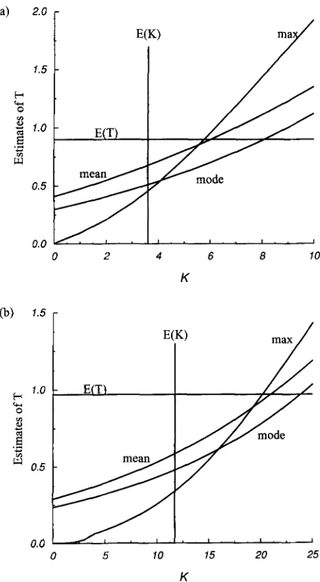
3, these estimators become too compli- cated to be derived analytically. Therefore, we compared the numerical values of these estimators for a number of combinations of n , K and 8. Figure 4 gives

two examples of the values these estimators. Figure 4a corresponds to 8 = 2 and sample size 10, and Figure 4b corresponds to 0 = 5 and sample size 30. The pattern of the values of the three estimators in a and b, as well as those in many other parameter settings not shown here, enable us to conclude that

1. The value of each of the three estimators increases with K .

2. For any values of 8 and sample size n ,

Lode

is smaller than

Lean.

This is because the posterior probability of Tis skewed to the left.

3. The maximum likelihood estimate Lax is equal to zero when K = 0 and is the smallest among the three estimators when K is small.

4. The value of the maximum likelihood estimator f,, increases with K most rapidly and eventually becomes the largest among the three estimators after

K is larger than a value that is larger than E ( K )

.

Interval estimate of T: Besides the two Bayesian point estimators &,ode and tmean, one can construct inter-

val estimates of T from the posterior probability

p,

( TI K )

.

For example, the 95% interval estimate of T

1.5

0.5

0.0

0 2 4 6 8 10

K

F. 1.0

0.0

0 5 15 10 20 25

K

FIGURE 4.-Estimates of T for given values of K . ( a ) n =

10 and 0 = 2; ( b ) n = 30 and 0 = 5.

can be defined as ( T2.5, T97.5), where T, is the value of

S such that

where

sos

p,

( K , t ) dt can be shown to be

k = 2 1=0

l ! k l - i - l

S C i e - k ( B + k - l ) S

,=O

( Z -

i ) ! ( 8

+

k - 1)"+'

Obviously T2,5 should be smaller than T97.5.

(7)

Estimating the Age of MRCA a35

4.0

r

b

2

3.0

d

a)

C

k

8

2.0

8

3

CI .e -a rF: C

2

1.0 Q\

0.0

0.0 0.25 0.5 0.75 1.0

KK99

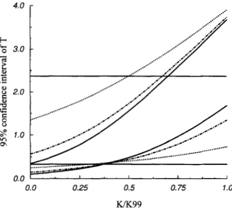
FIGURE 5.-The 95% interval estimate of Tfor a sample of 50 sequences. The two dotted lines, dashdotted lines and solid lines correspond to the upper and lower limits of the interval estimate for 6' = 1, 5 and 10, respectively; the two

horizontal lines correspond to the interval estimate based on the prior distribution, & ( T ) , of T . K99 is the number of segregating sites such that

p

( K 5 K99

1 6 ' )

=

0.99. The values

of K99 for 6' = 1, 5 and 10 are 12, 46 and 90, respectively.

T implies better estimate of T, Figure 5 concurs with our earlier analysis of the correlation coefficient between K and T. Figure 5 also shows that a large 8 im- proves mainly the estimate of the upper bound of T when K is small and the lower bound of T when K is large.

AN EXAMPLE: THE HUMAN Y CHROMOSOME

We shall consider the sample of DNA sequences by DORIT et al. ( 1995) from an intron of Z I T gene in the human Y chromosome. The sample consists of 38 sequences of 738 base pairs and has no sequence variation ( K = 0 )

.

Since Fu and LI ( 1996) (also see DON-

NELLY et al. 1996, WEISS and VON HAESELER 1996) have already analyzed this sample, we shall give a supplemen- tary analysis below.

To estimate the age of the MRCA of this sample, one has to obtain an estimate of the value of 8 = 2N&. Because homologous DNA sequences from several pri- mates were also available, DORIT et al. ( 1995) estimated the mutation rate per sequence per years as 0.98 X

Assume 20 years as one human generation, the mutation rate ( p ) per sequence per generation is thus 1.96 X 10 - 6 . In additions to the value of p, we need to

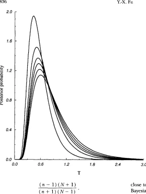
know the value of N,. Figure 6 shows the curves of the posterior probability for several values of

N,.

One can see that a larger value of

N,

results in a more concen- trated distribution of T. If one fixes the value of

N,

and varies the value of p, the effect on the posterior probability would be the similar to that shown in Figure

5. In other words, with increasing mutations rate, the posterior probability distribution will be more concen- trated, therefore the inference on Twill be more accu- rate.

Assuming equal sex ratio, FU and LI (1996) took

N,

= 5000 according to TAKAHATA ( 1993). This results in 8 = 0.196. Fu and LI (1996) obtained Lode = 114,000

yr,

Lean

= 174,000 yr and the 95% interval estimate of T is from 60,000 to 408,000

yr.

The maximum likelihood estimate

Lax

of Tis equal to zero as pointed out earlier. One can also compute the Bayesian estimates

Lode

and

Lea,,

and the 95% interval estimate of T directly from the prior distribution +n ( T )

.

This yields that L o d e

= 124,000,

Lea,

= 195,000 yr and the 95% interval estimate of T from 65,000 to 473,000 yr. Comparing these point estimates to those based the posterior probability distribution, we can see that the former are smaller. The interval estimate of T based on the posterior probability, which is a better indicator of the quality of the information in the sample, is 60,000 yr narrower than that based on the prior distribution of T. The improvement is apparently significant though not dra- matic, which is not surprising for two reasons. First, when

t9

= 0.196 the correlation coefficient between K

and Tis 0.25; therefore, the value of K provides only a modest amount of informative about T. Second, one can compute the probability of no variation from ( 2 0 ) , and with 8 = 0.196 this probability is 0.42, which is not small at all. Therefore, the posterior distribution of T is not too different from the prior distribution of T, which is equivalent to the posterior probability of T with 8 = 0.

Since our analytical results are derived under the WRIGHT-FISHER model with a constant effective population size and since the human population is apparently subdivided and is growing, the above analysis should be viewed as preliminary. However, NEI and TAKAHATA

( 1993) showed that, when population subdivision is not substantial ( i e . , 4 M m is not too small where m is the migration rate), the formula, 4N( 1 - 1

/

n )

,

of the mean age of the MRCA of a sample from a random mating population is also a good approximation to that of a sample from a subdivided population with N re- placed by the effective population size of the subdivided population. Therefore, the theory and estimators developed in this paper should be an usefu! starting point for the inferences on T.

DISCUSSION

We have focused on the age of the MRCA of a sample from a population. It is often more interesting to be able to estimate the age of the MRCA of a population, such as the cases of the human mitochondria and Y

(8)

2.0

1.6

-

h

‘1

. d 1.2

%

8

b

r,

E

. d

*

a 0.8

0.4

0.0

0.0 0.6 1.2 1.8 2.4

T

( n - 1 ) ( N + 1 )

( n

+

l ) ( N - 1 )

.

Because sample size is usually much smaller than the effective population size N , the above probability is ap- proximately equal to ( n - 1 )

/

( n

+

1 )

.

It follows that when n is large, it is reasonable to treat the MRCA of a sample as that of a population. For example, the probability that the MRCA of a random sample of 38 sequences is the same as the MRCA of a population is 0.95. Therefore, it is reasonable to treat the estimate of the age of the MRCA of the sample by DORIT et al. ( 1995) as that of the male human population, although one would feel safer if the sample size had been 100, which gives 0.98 probability that the two MRCAs are the same.

We presented in this paper three point estimators of T and showed that their values for a given sample are usually different. In particular, the maximum likelihood estimate can be substantially different from the two Bayesian estimates Lode and LC,,. This raises

the question on which of the three estimators should be preferred. As we have seen that when there is no variation in a given sample, the maximum likelihood estimate tax of T is 0, which is by all means a bad estimate. The maximum likelihood estimator ignores the fact that T has a bell-shaped distribution so that it is unlikely to be either too small or too large and thus yields estimates that seems to be too small when K is

FIGURE 6.-Posterior probability

p,(

TIO) with different effective population sizes for a sam le of 38 sequences, given that p = 0.98 X

10-

P

X 20. The curves with descending peaks correspond to N , = 30,000, 15,000,10,000,7500, 5000 and 2500, respectively.

3.0

close to zero and too large when K is large. Therefore, Bayesian estimates should be preferred over the maximum likelihood estimate of T from the value of K.

Between the two Bayesian estimators,

Lode

should be preferred over

Le,,,

because the former is the most likely value of T for the given value of K while the latter is the average value of T. When one has to draw conclusions about T from a single sample, the average value of T appears to be less relevant. However, this judgment is necessarily subjective to some extent and I

recommend to report the values of all the three estimators when analyzing real samples.

We also presented an interval estimate of T derived from the posterior probability distribution of T. It should be emphasized that the resulting 95% interval of Tis not the 95% confidence interval of any of the three point estimators discussed in this paper. This fact can be overlooked easily and when the phrase “interval of T” is used loosely, it is tempting to interpret it as the confidence interval of a point estimator, although the two intervals should be correlated. Because the interval estimate of Tallows one to make a very informative probabilistic statement, such as, with 0.95 probability Tis in a certain interval, I strongly recommend the use of interval estimate of T .

(9)

Estimating the Age of MRCA 837

ing that the accuracy in the estimation of

8

from K

increases with the value of 8 ( FELSENSTEIN 1992; FU and LI 1993a). Because we assume that

8

is known in this paper, while in reality the same sample will proba- bly be used to estimate both 8 and T , a sample of DNA sequences from a locus with large value of 8 will improve the estimations of both

8

and T .

Finally, it has been demonstrated that phylogenetic information in a sample can improve the accuracy in the estimation of 8 ( e.g., FU 1994) ; it is thus of interest to explore the possibility of incorporating phylogenetic information in a sample into the estimation of the age of the MRCA of the sample. One such approach has been developed by GRIFFITHS and TAVARE ( 1994). The extent of the improvement of inference by such approaches remains to be seen, but the estimation of the age of the MRCA based on the number of segregating sites should be efficient at least for DNA samples with few segregating sites.

I thank Drs. J. FEISENSTEIN, W. H. LI and N. TAKAHATA, and a reviewer for their commens and suggestions. This research was sup- ported by National Institutes of Health grant R29 GM-50428.

LITERATURE CITED

DONNELLY, P., S. TAVARE, D. J. BALDING and R. C . GRIFFITHS, 1996 Estimating the age of the common ancestor of mem from the ZFYintron. Science 272: 1357-1359.

DORIT, R. L., H. AKASHI and W. GILBERT, 1995 Absence of polymorphism at the ZFYlocus on the human Y chromosome. Science FELSENSTEIN, J., 1992 Estimating effective population size from samples of sequences: inefficiency of pairwise and segregation sites as compared to phylogenetic estimates. Genet. Res. 56: 139-147. Fu, Y . X., 1994 A phylogenetic estimator of effective population size

or mutation rate. Genetics 136: 685-692.

Fu, Y . X., 1996 New statistical tests of neutrality for DNA samples from a population. Genetics 143: 557-570.

Fu, Y . X., and W. H. LI, 1993a Maximum likelihood estimation of population parameters. Genetics 134 1261 -1270.

Fu, Y . X., and W. H. LI, 1993b Statistical tests of neutrality of mutations. Genetics 133: 693-709.

Fu, Y . X., and W. H. Lr, 1996 Estimating the age of the common ancestor of mem from the ZFYintron. Science 2 7 2 1356-1357. GRIFFITHS, R. C., and S. TAV&, 1994 Ancestral inference in popula-

tion genetics. Stat. Sci. 9 307-319.

HUDSON, R. R., 1983 Properties of a neutral allele model with intra- genic recombination. Theor. Pop. Biol. 23: 183-201.

KIMuRA, M., 1970 The length of time required for a selectively neu-

tral mutant to reach fixation through random frequency drift in a finite population. Genet. Res. 15: 131-133.

KINGMAN, J. F. C., 1982a The coalescent. Stochastic processes and

their applications. 13: 235-248.

KINGMAN, J. F. C., 1982b On the genealogy of large populations. J.

Appl. Probab. 19A: 27-43.

NEI, M., and N. TAKAHATA, 1993 Effective population size, genetic diversity, and coalescent time in subdivided populations. J. Mol. Evol. 37: 240-244.

SAUNDERS, L. W., S. TAV& and G. A. WATTERSON, 1984 O n the genealogy of nested subsamples from a haploid population. Adv. Appl. Prob. 16: 471-491.

TAJIMA, F., 1983 Evolutionary relationship of DNA sequences in finite populations. Genetics 105: 437-460.

TAJIMA, F., 1989 Statistical method for testing the neutral mutation hypothesis by DNA polymorphism. Genetics 123: 585-595. TAJIMA, F., 1990 Relationship between DNA polymorphism and fix-

ation time. Genetics 125: 447-454.

268: 1183-1185.

TAKAHATA, N., 1993 Allelic genealogy and human evolution. Mol. Biol. Evol. 10: 2-22.

TAV&, S., 1984 Line of descent and genealogical process and their applications in population genetics models. Theor. Popul. Biol.

WATTERSON, G. A,, 1975 On the number ofsegregation sites. Theor. Popul. Biol. 7: 256-276.

WEISS, G., and A. VON HAESELER, 1996 Estimating the age of the

common ancestor of mem from the ZFY intron. Science 272:

1359-1360.

26: 119-164.

Communicating editor: N. TAKAHATA

APPENDIX: DERIVATION OF

p,(

K , T ) Let

gk = k(I3

+

k - 1 ) T k = T - t,-

...

- tk

2- 1

L ( k , i) = kT+ ( j - k ) t , ,

j = 2

and

2- 1

G ( k , 2) = g J

+

c

( g r -

g d t j .

j = 2

Because of the constraint &

+

* *

+

tn = T , t, is

equal to T,-,

.

It follows that Equation 4 can be written as

S,

L K ( ~ , n ) e - G ( n , n ) r,t- 2

dtn-I ,

.

dt,

which can be computed by integrating with respect to

t n - l ,

. . .

, & in turns. Note that it is equivalent to write

L K ( n , n ) e - G ( n , n ) as n K

fn-l = akl( n ) ~ ' ( k , n ) e - G ( k , n ) ,

k =n Is0

where

a n K ( n ) = 1, (Y,O ( n ) = * *

.

= (Y,K-I ( n ) = 0. (28) Suppose that the function to be integrated with respect to ti is

n K

= a k , ( i + l ) L ' ( k , i + l ) e - c ( k " + l ) .

k = t + I 1=0

Then because

d ' L 1 ( k , i

+

1 ) - Z ! ( i - k)'

dt{ ( 1 -

j ) !

- L l - J ( k , i

+

1 ) ,

(10)

where

k =

i +

1 ,

. . . ,

n

a i l ( i ) =

-

a k l ( i ) ( 2 9 ) R=i+l

for 1 = 0 ,

.

. .

, K .

The last integration with respect to

4

yields

X ( k ~ ) l e - k ( o + k - l ) T

( 3 0 )

Therefore,

pn

( K , T ) can be calculated from (30 ) once we know the values of &( 2 ) , which can be obtained sequentially from the iteration ( 2 9 ) with initial condi- tions given by (28)