A Compressive Sensing Based Approach to Sparse Wideband Array Design

Array Design

.

White Rose Research Online URL for this paper:

http://eprints.whiterose.ac.uk/94834/

Other:

Hawes, M.B. and Liu, W. (2014) A Compressive Sensing Based Approach to Sparse

Wideband Array Design. UNSPECIFIED. (Unpublished)

[email protected] https://eprints.whiterose.ac.uk/ Reuse

Unless indicated otherwise, fulltext items are protected by copyright with all rights reserved. The copyright exception in section 29 of the Copyright, Designs and Patents Act 1988 allows the making of a single copy solely for the purpose of non-commercial research or private study within the limits of fair dealing. The publisher or other rights-holder may allow further reproduction and re-use of this version - refer to the White Rose Research Online record for this item. Where records identify the publisher as the copyright holder, users can verify any specific terms of use on the publisher’s website.

Takedown

If you consider content in White Rose Research Online to be in breach of UK law, please notify us by

arXiv:1403.4879v1 [cs.IT] 19 Mar 2014

A Compressive Sensing Based Approach to

Sparse Wideband Array Design

Matthew B. Hawes and Wei Liu Communications Research Group

Department of Electronic and Electrical Engineering University of Sheffield, UK

{elp10mbh, w.liu}@sheffield.ac.uk

Abstract—Sparse wideband sensor array design for sensor

location optimisation is highly nonlinear and it is traditionally solved by genetic algorithms, simulated annealing or other similar optimization methods. However, this is an extremely time-consuming process and more efficient solutions are needed. In this work, this problem is studied from the viewpoint of compressive sensing and a formulation based on a modifiedl_{1norm is derived.}

As there are multiple coefficients associated with each sensor, the key is to make sure that these coefficients are simultaneously minimized in order to discard the corresponding sensor locations. Design examples are provided to verify the effectiveness of the proposed methods.

Index Terms—Sparse array, frequency invariant beamforming,

wideband beamforming, tapped delay-line, compressive sensing.

I. INTRODUCTION

Wideband beamforming has been studied extensively in the past [1], [2]. It is well-known that in order to avoid the spatial aliasing problem for uniform linear arrays (ULAs), the adjacent sensor spacing has to be less than half of the minimum operating wavelength corresponding to the highest frequency of the signal of interest. On the other hand, sparse arrays allow adjacent sensor separations greater than half a wavelength while still avoiding grating lobes due to the randomness of sensor locations [3].

However, the unpredictable sidelobe behaviour associated with sparse arrays means some optimisation of sensor loca-tions is required to reach an acceptable performance level. Various nonlinear methods have been used to achieve this required optimisation. For example, Genetic Algorithms (GAs) [4], [5], [6] and Simulated Annealing (SA) [7] have been regularly used. The disadvantage of these types of methods are the potentially extremely long computation times and the possibility of convergence to a non-optimal solution.

Recently, the area of compressive sensing (CS) has been explored [8], and CS-based methods have been proposed in the design of narrowband sparse arrays [9], [10], [11], [12]. Further work has also shown that it is possible to improve the sparseness of a solution by considering a reweighted l1 minimisation problem [13], [14], [15], [16]. The aim of these methods is to bring the minimisation of the l1 norm of the weight coefficients closer to that of the minimisataion of the

l0 norm.

However, for a wideband array to be sparse, all coeffi-cients along the tapped delay-lines (TDLs) associated with

[n]

s Ts

w

w

w

T_s T_s

x0[n]

M−1

d

w

w

w

y[n]

θ θ

M−1,0

xM−1

T

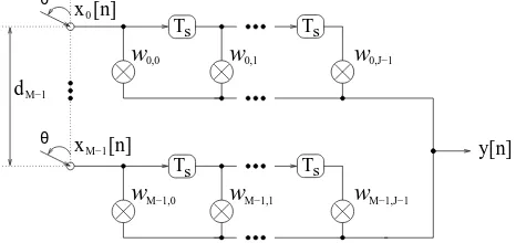
Fig. 1. A general wideband beamforming structure with a TDL lengthJ.

an individual sensor have to be equal or very close to zero. Therefore, it is not sufficient to simply minimize thel1norm of the weight coefficients. Instead, a method similar to the tech-nique employed in complex-valuedl1norm minimization [17], is presented in this paper, which can be considered as an expanded version of the idea in [18]. As in the case with narrowband array design, it is possible to use a reweighted scheme for the wideband method as well.

The remainder of this paper is structured as follows. Sec. II gives details of the array model, followed by the proposed design methods in Sec. III. Design examples are provided in Sec. IV and conclusions are drawn in Sec. V.

II. WIDEBANDARRAYMODEL

A general linear array structure for wideband beamforming with a TDL length J is shown in Fig. 1, where Ts is the sampling period or temporal delay between adjacent signal samples [2]. The beamformer output y[n] is a linear combi-nation of differently delayed versions of the received array signals xm[n], m = 0,· · ·, M −1. The distance from the zeroth sensor to the subsequent sensor is denoted bydm for

m= 0,· · ·, M −1, where d0= 0 as it is the distance from the zeroth sensor to itself.

The steering vector of the array as a function of the normalized frequency Ω = ωTs and the angle of arrival θ is

s(Ω, θ) = [1,· · ·, e−jΩ(J−1)_,

e−jΩµ1cos(θ)_{, e}−jΩ(µ1cos(θ)+1)_,

· · · , e−jΩ(µ1cos(θ)+(J−1))_,

· · · , e−jΩ(µM₋₁cos(θ)+(J₋1))

]T. (1)

whereµm=_cTdms form= 0,1,· · ·, M−1and{·}

T _indicates

transpose operation.

The response of the array is then given by

P(Ω, θ) =wHs(Ω, θ), (2)

where wH is the Hermitian transpose of the weight coefficient vector of the array, given by

with

wm= [wm,0 wm,1 ... wm,J−1]T. (4)

III. SPARSEWIDEBANDARRAYDESIGN VIA

COMPRESSIVESENSING

As previously mentioned, CS has been employed in the de-sign of sparse narrowband arrays by trying to match the array’s response to a desired/reference one, Pr(Ω, θ). Extending the design to the wideband case, we first consider Fig. 1 as being a grid of potential active sensor locations. In this instance,dM−1

is the maximum aperture of the array and the values ofdm, for

m= 1,2, . . . , M−2, are selected to give a uniform grid, with

M being a large enough number to cover all potential locations of the sensors. Sparseness is then introduced by selecting the set of weight coefficients to give as few active locations as possible, while still giving a designed response that is close to the desired one.

In the first instance, this problem could be formulated as

min ||w||0

subject to ||p_r−wHS||2≤α , (5)

where||w||0is the number of nonzero weight coefficients in w,

p_ris the vector holding the desired beam response at sampled frequency points Ωk and angle θl, k = 0,1,· · ·, K −1,

l= 0,1,· · ·, L−1, S is the matrix composed of the steering vectors at the corresponding frequency Ωk and angle θl, and

αplaces a limit on the allowed difference between the desired and the designed responses. In the constraint in (5) ||.||2 denotes the l2 norm.

In detail, p_rand S are respectively given by

p_r = [Pr(Ω0, θ0),· · ·, Pr(Ω0, θL−1),

Pr(Ω1, θ0),· · ·, Pr(Ω1, θL−1)

..., Pr(ΩK−1, θL−1)]

and

S = [s(Ω0, θ0),· · · ,s(Ω0, θL−1),

s(Ω1, θ0),· · · ,s(Ω1, θL−1),· · ·,s(ΩK−1, θL−1)].

Here the desired responsePr(Ω, θ)can be obtained from that of a traditional uniform linear array, or simply assumed to be an ideal response (i.e. one at the mainlobe area and zero for the sidelobe area) and this is adopted in what follows.

In practice, the cost function in (5) will be replaced by the

l1 norm,

min ||w||1

subject to ||p_r−wHS||2≤α . (6)

The above formulation is effective in the design of narrow-band arrays, where the TDL length J = 1 (i.e. each sensor has only one weight coefficient attached) and the number of nonzero coefficients will be the same as the number of active sensors. In other words, any coefficient with a zero value

will mean that the associated sensor is inactive. However, in the wideband case, to guarantee a sparse solution, the weight coefficients along a TDL have to be simultaneously minimized. When all coefficients along a TDL are zero-valued, we can then consider the corresponding location to be inactive and sparsity is introduced. To achieve this, similar to the technique used in complex-valuedl1norm minimization [17], we minimize a modified l1 norm as follows [18],

min t ǫ R+

subject to ||p_r−wHS||2≤α

|hwi|1≤t (7)

where

|hwi|1= M−1

X

m=0



 

wm,0 .. .

wm,J−1



  ₂

. (8)

Now we decomposettot=PM−1

m=0tm,tmǫ R+. In vector form, we have

t= [1,· · · ,1]



 

t0 .. .

tM−1



 =1

T_{t. (9)}

Then (7) can be rewritten as

min

t 1

T_t

subject to ||p_r−wHS||2≤α



 

wm,0 .. .

wm,J−1



 

2

≤tm, m= 0,· · ·, M−1.

(10)

Now define

ˆ

w= [t0, w0,0,· · ·, w0,J−1, t1,· · · , wM−1,J−1]

T_{, (11)}

ˆ

c= [1,0J,1,0J,· · ·,0J]T (12)

and

ˆs(Ω, θ) = [0,1,· · ·, e−jΩ(J−1)_,

0, e−jΩµ1cos(θ)_{, e}−jΩ(µ1cos(θ)+1)_{,· · · ,}

e−jΩ(µ1cos(θ)+(J−1))_,

· · ·, e−jΩ(µM₋₁cos(θ)+(J₋1))

]T, (13)

where 0J is an all-zero1×J row vector. A matrixS similarˆ to (6) can be created fromˆs, given by

ˆ

S = [ˆs(Ω0, θ0),· · ·,ˆs(Ω0, θL−1),

Finally we arrive at the final formulation for the sparse wideband sensor array design problem

min ˆ

w ˆc

T_wˆ

subject to ||p_r−wˆHSˆ||2≤α

  

wm,0 .. .

wm,J−1

   2

≤tm, m= 0,· · · , M−1.

(14)

In the above formulation, it is straightforward to add addi-tional constraint to meet some specific design requirements. For example, we can add the response variation constraint

RV =||LTwˆ||2

2≤σ2 derived in [22], [23] to design a sparse wideband array with frequency invariant beam response [19], [20], [21], [22], where the matrix L and the threshold value

σ are formulated to make sure the change of response of the resultant beamformer with respect to different frequencies is limited to an acceptable level.

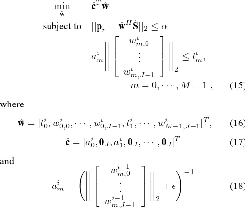
Moreover, to increase sparsity of the resultant array, we can adopt the reweighted l1 minimisation approach in [16] and reformulate (14) into the following form

min ˆ

w ˆc

T_ˆ w

subject to ||p_r−wˆHˆS||2≤α

ai_m

   wi m,0 .. .

wi_m,J−1

   2 ≤ti_m,

m= 0,· · · , M−1, (15)

where

ˆ

w= [ti0, wi0,0,· · ·, w0i,J−1, t

i

1,· · ·, wMi −1,J−1]

T_{, (16)}

ˆc= [ai0,0J, a1i,0J,· · ·,0J]T (17)

and

ai_m=   

wi−1

m,0 .. .

wi−1

m,J−1

   ₂ +ǫ

!−1

(18)

Here ǫ >0andi is the iteration number.

The above problem can be solved using cvx, a package for specifying and solving convex programs [24], [25].

IV. DESIGNEXAMPLES

In this section design examples are presented, which were all implemented on a computer with an Intel Core Duo CPU E6750 (2.66GHz) and 4GB of RAM. Comparisons will be drawn with a GA-based design method, which optimises the locations given a fixed number of sensors. In the GA based design, the fitness value was chosen to beJ−1

CLS, whereJCLS is defined in [22].

In the following example, the reference pattern was that of an ideal array with the mainlobe at θm = 90◦ and sidelobe

TABLE I

SENSORLOCATIONSFORTHEREWEIGHTEDBROADSIDEDESIGN

EXAMPLE.

n dn/λ n dn/λ

0 1_.92 ₆ 5_.66

1 2_.83 ₇ 6_.26

2 3_.33 ₈ 6_.67

3 3_.74 ₉ 7_.17

4 4_.34 ₁₀ 8_.08

5 5_.00

0 20 40 60 80 100 120 140 160 180

−70 −60 −50 −40 −30 −20 −10 0

θ (degrees)

Beam pattern (dB)

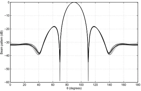
Fig. 2. Responses for reweighted broadside design example.

regions ofΘs= [0◦_,80◦_]S

[100◦_,180◦_{], which were sampled}

every1◦_{. The frequency range of interestΩI = [0.5π, π] was}

sampled every0.05π, with the reference frequency Ωr =π. A grid of100potential sensor locations was spread uniformly over an aperture of10λ, where the value ofλis the wavelength associated with a normalized frequency ofΩ =π. The values

α= 0.9,σ = 0.01, ǫ= 9×10−4 _{and TDL length J = 25}

were used.

The resulting array using the reweighted method was made up of 11 active sensor locations as given in Tab. I, with its beam response shown in Fig. 2. It can be seen that the mainlobe is at the desired location for each normalised frequency and sufficient attenuation has been achieved in the sidelobe regions. The response also shows a good level of performance in terms of the FI property.

This was then compared to an array designed using the GA-based method. To allow a fair comparison, the GA was set to optimise11sensor locations over an aperture of 6.16λ, the same as the example given in Tab. I. Fig. 3 shows the resulting array response.All these show a good performance in terms of both sidelobe attenuation and the FI property.

0 20 40 60 80 100 120 140 160 180 −60

−50 −40 −30 −20 −10 0

θ (degrees)

Beam pattern (dB)

Fig. 3. Responses for the GA broadside design example.

TABLE II

BROADSIDEPERFORMANCECOMPARISON.

Method Reweighted GA Mean Spacing/λ 0.62 0.62

JCLS 0.0372 0.0376

Computation Time (minutes) 130 436

lower for reweighted CS designed array, suggesting that in this instance the reweighted wideband CS method has provided a more desirable response (the difference largely being the FI property in the extremes of the sidelobe regions). This will not be guaranteed to be the case all the time.

V. CONCLUSIONS

In this paper, a CS-based method for the design of sparse wideband arrays has been proposed, where a modifiedl1norm minimization problem is derived to simultaneously minimize the coefficients along a tapped delay-line associated with each sensor. Extra constraints can then be added to meet the specific design requirements, such as the frequency invariant constraint. To further improve the sparsity of the final design result, an iterative process is employed with a reweighting term introduced in the cost function. Design examples have been presented, with comparisons also drawn with a GA-based method. Similar performance levels are achieved but the GA design takes considerably longer to reach the solution, highlighting the advantage of our proposed design methods.

REFERENCES

[1] H. L. Van Trees, Optimum Array Processing, Part IV of Detection,

Estimation, and Modulation Theory. New York, U.S.A.: John Wiley & Sons, Inc., 2002.

[2] W. Liu and S. Weiss, Wideband Beamforming: Concepts and Techniqeus. Chichester, UK: John Wiley & Sons, 2010.

[3] P. Jarske, T. Saramaki, S. K. Mitra, and Y. Neuvo, “On properties and design of nonuniformly spaced linear arrays,” IEEE Transactions on

Acoustics, Speech, and Signal Processing, vol. 36, no. 3, pp. 372 –380,

March 1988.

[4] R. L. Haupt, “Thinned arrays using genetic algorithms,” IEEE

Transac-tions on Antennas and Propagation, vol. 42, no. 7, pp. 993–999, July

1994.

[5] K.-K. Yan and Y. Lu, “Sidelobe reduction in array-pattern synthesis using genetic algorithm,” IEEE Transactions on Antennas and

Propa-gation, vol. 45, no. 7, pp. 1117 –1122, July 1997.

[6] M. B. Hawes and W. Liu, “Location optimisation of robust sparse antenna arrays with physical size constraint,” IEEE Antennas and

Wireless Propagation Letters, pp. 1303–1306, November 2012.

[7] A. Trucco and V. Murino, “Stochastic optimization of linear sparse arrays,” IEEE Journal of Oceanic Engineering, vol. 24, no. 3, pp. 291– 299, July 1999.

[8] E. Candes, J. Romberg, and T. Tao, “Robust uncertainty principles: exact signal reconstruction from highly incomplete frequency information,”

IEEE Transactions on Information Theory, vol. 52, no. 2, pp. 489 –

509, February 2006.

[9] L. Li, W. Zhang, and F. Li, “The design of sparse antenna array,” CoRR, vol. arXiv.org/abs/0811.0705, 2008.

[10] G. Prisco and M. D’Urso, “Exploiting compressive sensing theory in the design of sparse arrays,” in Proc. IEEE Radar Conference, May 2011, pp. 865 –867.

[11] L. Carin, “On the relationship between compressive sensing and random sensor arrays,” IEEE Antennas and Propagation Magazine, vol. 51, no. 5, pp. 72 –81, October 2009.

[12] M. B. Hawes and W. Liu, “Robust sparse antenna array design via compressive sensing,” in Proc. International Conference on Digital

Signal Processing, July 2013.

[13] E. J. Candes, M. B. Wakin, and S. P. Boyd, “Enhancing sparsity by reweightedl1minimization,” Journal of Fourier Analysis and

Applica-tions, vol. 14, pp. 877–905, 2008.

[14] B. Fuchs, “Synthesis of sparse arrays with focused or shaped beam-pattern via sequential convex optimizations,” IEEE Transactions on

Antennas and Propagation, vol. 60, no. 7, pp. 3499 –3503, july 2012.

[15] G. Prisco and M. D’Urso, “Maximally sparse arrays via sequential con-vex optimizations,” IEEE Antennas and Wireless Propagation Letters, vol. 11, pp. 192 –195, 2012.

[16] M. B. Hawes and W. Liu, “Compressive sensing based approach to the design of linear robust sparse antenna arrays with physical size constraint,” IET Microwaves, Antennas & Propagation, 2014, DOI: 10.1049/iet-map.2013.0469.

[17] S. Winter, H. Sawada, and S. Makino, “On real and complex valuedl1

-norm minimization for overcomplete blind source separation,” in Proc.

of IEEE Workshop on Applications of Signal Processing to Audio and Acoustics, October 2005, pp. 86 – 89.

[18] M. B. Hawes and W. Liu, “Sparse microphone array design for wideband beamforming,” in Proc. International Conference on Digital Signal

Processing, July 2013.

[19] W. Liu, S. Weiss, J. G. McWhirter, and I. K. Proudler, “Frequency in-variant beamforming for two-dimensional and three-dimensional arrays,”

Signal Processing, vol. 87, pp. 2535–2543, November 2007.

[20] W. Liu and S. Weiss, “Design of frequency invariant beamformers for broadband arrays,” IEEE Transactions on Signal Processing, vol. 56, no. 2, pp. 855–860, February 2008.

[21] W. Liu, D. McLernon, and M. Ghogho, “Design of frequency invariant beamformer without temporal filtering,” IEEE Transactions on Signal

Processing, vol. 57, no. 2, pp. 798–802, February 2009.

[22] Y. Zhao, W. Liu, and R. J. Langley, “An application of the least squares approach to fixed beamformer design with frequency invariant constraints,” IET Signal Processing, vol. 5, pp. 281–291, June 2011. [23] ——, “Adaptive wideband beamforming with frequency invariance

constraints,” IEEE Transactions on Antennas and Propagation, vol. 59, no. 4, pp. 1175–1184, April 2011.

[24] C. Research, “CVX: Matlab software for disciplined convex program-ming, version 2.0 beta,” http://cvxr.com/cvx, September 2012. [25] M. Grant and S. Boyd, “Graph implementations for nonsmooth convex