A Fast Algorithm for Finding Correlation Clusters
in Noise Data
Jiuyong Li1, Xiaodi Huang2, Clinton Selke3, and Jianming Yong4
1
School of Computer and Information Science, University of South Australia, Mawson Lakes
Adelaide, Australia, 5095
2
Department of Mathematics, Statistics and Computer Science, The University of New England, Armidale, Australia, 3
Department of Mathematics and Computing, The University of Southern Queensland,
Australia,
4
Department of Information Systems, University of Southern Queensland, Australia,
Abstract. Noise significantly affects cluster quality. Conventional clustering meth-ods hardly detect clusters in a data set containing a large amount of noise. Pro-jected clustering sheds light on identifying correlation clusters in such a data set. In order to exclude noise points which are usually scattered in a subspace, data points are projected to form dense areas in the subspace that are regarded as cor-relation clusters. However, we found that the existing methods for the projected clustering did not work very well with noise data, since they employ randomly generated seeds (micro clusters) to trade-off the clustering quality. In this paper, we propose a divisive method for the projected clustering that does not rely on random seeds. The proposed algorithm is capable of producing higher quality correlation clusters from noise data in a more efficient way than an agglomer-ation projected algorithm. We experimentally show that our algorithm captures correlation clusters in noise data better than a well-known projected clustering method.
Keywords: generalised projected clustering, SVD decomposition.
1
Introduction
Clustering is a classical technique in computing and statistics. Noise deteriorates cluster quality significantly and prevents finding meaningful clusters when the amount of noise is big. It is difficult to distinguish noise data objects from normal ones when we do not have prior knowledge about the data. However, clustering can serve as the first step to explore such a data set with noise, particularly when the prior knowledge about the data is unavailable.
Generalised projected clustering sheds light on solving this problem by finding cor-related clusters. When data objects are projected to a data subspace using Singular Value Decomposition (SVD) or PCA, the correlation clusters are condensed to a small area
1
whereas noise data objects scatter across the projected space. Therefore, it is possible to separate correlated data objects from noise ones.
Most existing projected clustering methods use agglomeration methods to find cor-relation clusters. A big data set is randomly partitioned into a large number of mi-cro clusters, and then an agglomeration approach is used to group correlation clusters. When correlated data are split into a number of micro clusters, they themselves be-come noise too. This process of randomly generated seeds affects the quality of found clusters. When a process for noise elimination is employed, many data objects in the correlation clusters are removed before they are grouped into clusters. Some well known examples of generalized projected clustering are PROCLUS [2], ORCLUS [1],4C[4], CURLER algorithm [5] and HARP [7]. We do not consider axis-parallel projection methods, also called subspace clustering, such as CLIQUE [3], and EPCH [6].
Instead of agglomerating randomly generated micro clusters into final clusters, we partition a data set into clusters in a top-down manner. The key idea for such a divi-sive method is to find a suitable criterion for data partition. We capture the direction of the largest variance of data using the corresponding principle vector, thereby taking small risk of partition correlation clusters into separate clusters. We employ grouping technique used in agglomeration methods to group correlation clusters after partitions. The proposed divisive projected clustering method preserves the essence of projected clustering, overcoming the drawbacks of existing projected clustering methods. In ad-dition, the proposed algorithm is significantly more efficient than most agglomeration algorithms.
2
Problem definitions
Projected clustering searches for hidden subspaces together with a set of data objects such that data objects are closed with each other in the lower dimensional subspaces. The hidden data spaces are found by using SVD decomposition. Eigenvectors corre-sponding to eigenvalues with low spreads forms a subspace. The intuitive explanation for this is as follows ( see more justifications in Section 4). When the covariance matrix of a set of correlated points is decomposed by SVD, some eigenvalues should be zero or close to zero. All the points are projected along a line in the subspace spanned by eigenvectors corresponding to these zero eigenvalues. In other words, the tightness of objects in the subspace defined by eigenvectors associated with the lowest eigenvalues is an alternative to measuring the correlation level of data objects.
Formally, letD be a dataset ofm data objects (row vectors) being treated asd -dimensional feature (column) vectors.oi ∈ D stands for thei-th object inDwhere
oi= (oi1, oi2, . . . , oid). Simply, we haveD= [oij],1≤i≤m, and1≤j≤d.
Definition 1. Generalised projected clustering
Given the user-specifiedlandk, a data setDis partitioned intokdisjoint subsetsD1,
Data points are clustered based on their closeness in some projected subspaces in-stead of the original space. This clustering captures correlations among data points.
To measure the closeness of data points in a subspace, the projected distance is defined as following.
Definition 2. Projected distance
LetDpbe a subset of a dataD.UpSpVpT = cov(Dp)(cov(Dp)is thed×dcovariance matrix ofDp, and Up, Sp,and VpT are results of SVD decomposition). LetE be the set of eigenvectors corresponding tol smallest eigenvalues. A data object p ∈ D is projected toE = (e1,e2, . . . ,el)space as(p·e1,p·e2, . . . ,p·el). The projected distance of objectspandq, denoted byPdist(p,q, E),is their Euclidean distance in projected spaceE.
The projected distance between two data points is the Euclidean distance between their projected images in a subspace. This distance varies in different subspaces.
To measure the projected distance variation over a group of data points in a sub-space, the projected energy is defined as the following.
Definition 3. Projected energy
The projected energy of data setDpis defined asEnergy(Dp, E) = Pi=N
i=1 Pdist(oi,c, E)/N,
whereN is the number of objects inDp,cthe centroid of all objects inDp, andEan associated subspace.
The smaller the projected energy, the denser the data point in the subspace. In clus-tering, low projected energy is preferred.
In projected clustering, the traditional distances between data objects are replaced by the projected distances in subspaces. However, there are no uniform and invariant distances in projected clustering since each tentative cluster has its own subspace. In other words, the distance between two objects varies in different subspaces.
Projected distances have been studied in statistics. The Mahalanobis distance [8] measures distance between two objects by using a set of reference data. But the Maha-lanobis distance is the projected distance in the entire space. The generalised projected distance is defined in a subspace, and is a generalised Mahalanobis distance.
As mentioned before, the ORCLUS algorithm [1] presents a variant agglomerative method to find kprojected clusters. First,D are randomly partitioned into k0 initial data subsetsD1,D2,. . .,Dk0, wherek0 >> k. If each data object is considered as an initial micro cluster, then the computational cost will be too expensive. The smaller
k0, the faster the ORCLUS. However, the high quality of clusters is sacrificed ifk0is small.
Second, ORCLUS performs the following two iterations:
1. Merge pairs of clusters with the smallest, combined project energy until the number of clusters is down tokp(determined by a parameter for the step sizeα).
The above procedure terminates untilkp = k with a parameterαto control the step size. If the step parameter is big, then a lot of merge occur in one iteration and the quality of final clusters is not guaranteed. If the step parameter is small, the execution time is increased.
A significant computational cost of the algorithm is from the decomposition of a data subsetDi. The complexity of such a decomposition is determined by the the num-ber of dimension (attributes). Specifically, it costsO(d3). Moreover, the computation has to be done in each merger of two data subsets. The complexity of the ORCLUS algorithm is therefore as high ask30+k0N d+k02d20.
A heuristic way of speeding up the ORCLUS algorithm is to makek0small and to conduct more merges in each step. However, the quality of clustering has been traded off. This problem is caused by the fact that ORCLUS is an agglomerative algorithm and too many merges are required to form a small number of clusters. In contrast, the divisive method needs much less steps to form clusters.
3
Divisive Projected clustering (DPCLUS)
Large computational costs of projected clustering lie in computing covariance matrixes and SVD (or PCA) decomposition. The computational costs of covariance matrixes and SVD (or PCA) decomposition is largely determined by the number of attributes,d, rather than the number of objects in a data setNi.
In most applications, we havek << mwheremis the number of objects in the data set, andkis the number of clusters. Therefore, a top-down method (divisive method) needs significantly less number of computations of covariance matrixes and SVD (or PCA) decomposition than a bottom-up one (agglomerative method).
A key question is how to partition the data. Given a dataset, the projected cluster problem can be regarded as the one of partition of the dataset intokclusters such that the sum of the projected distance of each data object to its cluster centroid is mini-mized. Compared to the clustering in full-dimensional space, the projected clustering makes use of the projected distance instead of the full-dimensional distance. Recall that we need to find a best subspace and their associated subsets of data objects such that the sum of the projected distances of data objects to their centroids is minimized. The number of the projected clusters in our algorithm is given. So it is to determine only the directions of spanning vectors. Within one cluster the optimal direction of the vector to which its associated data objects are projected should reflect the minimal variance of these data. An eigenvalue is numerically related to the variance it captures. The higher the value, the more variance it has captured. The principal vector defines a projection that encapsulates the maximum amount of variation in a dataset. This principal vector is in fact the eigenvector with the highest corresponding eigenvalue.
We make use of the principle vector of eigenvectors. All data objectsDare projected to the principle vector as discussed in the previous section, and the centroid separates data into two groups:D1andD2.D1contains data objects whose projected values are greater than or equal to the means, andD2contains the rest.
DPCLUS algorithm (Divisive Projected clustering)
Input: data setD, cluster numberk, subspace dimensionl, the minimum object numberminN, and the minimum distance for excluding outliersδ
Output:≥kprojected clusters
initialise an empty treeT;
let the root ofTstoreD;
where (the number of leaves ofT < k)
foreachDistored in a leaf of the newest layer Partition (Di);
Redistribute (all data sets stored in the leaves of the newest layer);
output data sets stored in all leaves ofT;
Function Partition(Di)
ifDisatisfies Definition 1 or|Di|<minN
then terminate the leaf storingDiand return;
splitDiintoDi1andDi2by the centroid in the principal vector;
insert two son leaves of the node storingDito storeDi1andDi2;
Function Redistribution(all data sets stored in the newest layer) foreach data object p in all data sets stored in the newest layer
foreach data setDjstored in the newest layer
compute the projected distance between p and the center of Dj;
if projected distances of p to all data sets> δ
then exclude p from future clustering;
else assign p to the data set with the smallest projected distance;
The DPCLUS algorithm partitions a data set into clusters in a top- down manner. The splitting point is the centroid of data objects projected to the principal vector. This saves a lot of computation for covariance matrixes and SVD decompositions as done in the ORCLUS algorithm. The sole dependence on the principal vector to separate data is rough and does not produce quality clusters. We design theRedistributionfunction to minimise the projected energy of each clusters after clusters are formed by partitions.
The number of final clusters can be greater thankbecause the number of leaves is not tested until all data sets stored in the newest tree layer are split and redistributed.
Outliers affect the quality of final clusters very much since they change the orien-tations of data objects greatly. Some data objects may not belong to any cluster and are considered outliers. To deal with this problem, we set an outlier threshold in Re-distribution step, sayδ. When the projected distance of a data object to any cluster is greater thanδ, then the data object is considered as an outlier and is excluded from the subsequent clustering.
We discuss the complexity of the algorithm in the following.
It is assumed that k denotes the number of final classes,N the number of data objects,dthe dimension of the data set, andlthe dimension of subspace.
After the partition, each cluster has to be decomposed again to determine whether or not it satisfies the projected clustering requirement. If no, it will participate in redis-tribution. The number of such decomposition is 2k, and hence the costs for the decom-positions is 2kd3. All clusters are projected toldimensional subspaces, and each data object has to be checked against each cluster. Therefore, the total costs for distribution iskN l.
In sum, the computational complexity for the DPCLUS algorithm is O(3kd3+
kN d). Note that we could not do much for termd3since it is for computing a covariance matrix and a SVD decomposition. However, the proposed algorithm has reduced the number of such computations significantly.
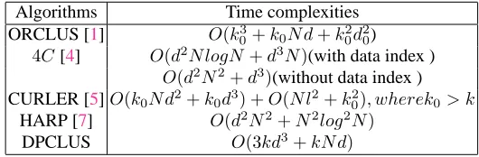
Our DPCLUS algorithm is faster than most exiting generalised projected clustering algorithms. We compare the time complexities in the table below.
Algorithms Time complexities
ORCLUS [1] O(k3
0+k0N d+k20d20)
4C[4] O(d2N logN +d3N)(with data index )
O(d2N2+d3)(without data index ) CURLER [5]O(k0N d2+k0d3) +O(N l2+k02), wherek0> k
HARP [7] O(d2N2+N2log2N)
DPCLUS O(3kd3+kN d)
It should be noted that in order to speed up, some algorithms make use of techniques such as heuristics, small number of micro-clusters, and random samples. However, these techniques come with a price; that is, some of the clustering quality must be sacrificed.
4
Experimental evaluation
4.1 Efficiency comparison to ORCLUS
We use synthetic data sets for this experiment. More details about how these data sets were generated will be given in the following subsection.
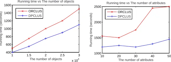
For the test of scalability with the size of data sets, the data sets each contain 10 attributes and up to 300,000 objects. For the test of scalability with the number of at-tributes, the data sets each contain 100,000 objects and up to 50 attributes. The number of embedded clusters is fixed to 20 for the above two tests.
lis set to 10 for both methods.k0is set to15×kto make ORCLUS efficient.δfor both methods is set as 0.01.minN varies for different data sets, but is set as the same for both methods. A value less than 0.0001 is consider as 0 in the experiments to test the satisfaction of Definition 1.
[image:6.595.174.439.273.360.2]1 1.5 2 2.5 3
x 104 400
600 800 1000 1200 1400 1600
Running time vs The number of objects
Running time (seconds)
The number of objects ORCLUS
DPCLUS
10 20 30 40 50
1000 1500 2000 2500
Running time vs The number of attributes
Running time (seconds)
The number of attributes ORCLUS
[image:7.595.153.453.117.226.2]DPCLUS
Fig. 1. The scalability of DPCLUS in comparison to that of ORCLUS
4.2 Clustering quality
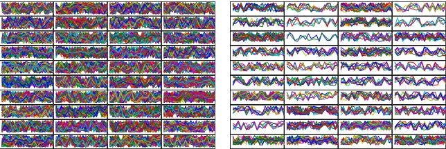
To demonstrate the clustering quality of DPCLUS, we compare it to three clustering methods on a synthetic data set. We embedded 20 clusters that are correlated in some subspaces over a set of random data objects. The data set contains 10,000 data objects, with each object having 20 attributes. Each embedded cluster contains 250 data ob-jects, which have 10% variations from the original pattern. Other 5,000 data objects are random data objects generated by the uniform distribution.
We set the parameters of DPCLUS asl = 10,k= 20,minN = 50, andδ= 0.01. The results from DPCLUS are shown in Figure2. DPCLUS is able to find all embedded clusters correctly. Althoughkis set as 20 in the experiment, the number of final clusters can be any integer number between 20 to 32, because the number of clusters is not tested until all data sets stored in the newest tree layer are split and redistributed. The number of the found clusters are greater than 20, since some clusters are split into two. For example, clusters at row 2: 1 and 2 are from the same cluster. DPCLUS has successfully identified cluster patterns from random data.
We set the parameters of ORCLUS ask = 20,l = 10,k0 = 350, andδ = 0.01. Figure2shows a good result. ORCLUS identified fewer than a half of embedded clus-ters with high quality. Since initial micro-clusclus-ters in ORCLUS is randomly chosen, the final clusters vary in different executions.
[image:7.595.141.474.564.641.2]We further show that both k-means and hierarchical clustering methods failed to find quality clusters in such noise data in Figure 3. Data is sampled for hierarchical clustering method because of efficiency constraint.
Fig. 3. Left: clusters found by kmeans. Right: Clusters found by hierarchical clustering.
5
Conclusions
We have presented a divisive, projected clustering algorithm for detecting correlation clusters in highly noised data. The distinction of noise points from correlated data points in a projected space offers benefits for projected clustering algorithms to discover clus-ters in noise data. The proposed algorithm mainly explores this potential. Further, the proposed algorithm is faster than most existing general projected clustering algorithms, which are agglomerative clustering ones. Unlike those agglomerative algorithms, the produced clusters by the proposed algorithm do not rely on the choice of randomly generated initial seeds, and are completely determined by the data distribution. We ex-perimentally show that the proposed algorithm is faster and more scalable than than ORCLUS, a well-known agglomerative projected clustering, and that the proposed al-gorithm detects correlation clusters in noise data better than ORCLUS.
References
1. C. C. Aggarwal and P. S. Yu. Finding generalized projected clusters in high dimensional spaces. In Proceedings of the 2000 ACM SIGMOD international conference on Management
of data (SIGMOD), pages 70–81, 2000.
2. C. C. Aggarwal, C. Procopiuc, J. L. Wolf, P. S. Yu, and J. S. Park. Fast algorithms for projected clustering. In Proceedings of the ACM SIGMOD Conference, pages 61-72, 1999.
3. R. J. Aggrawal, J. Gehrke, D.Gunopulos, and P. Raghavan. Automatic subspace clustering of high dimensional data for data mining applications. In Proceedings of the ACM SIGMOD
Conference, pages 94-105, 1998, Seattle, WA.
4. C. Bhm, K. Kailing, P. Krger, and A. Zimek. Computing Clusters of Correlation Connected objects. In Proceedings of the ACM SIGMOD international conference on Management of
data, June 13-18,2004, Paris, France.
5. A. K. H. Tung, X. Xu, and B. C. Ooi. CURLER: finding and visualizing nonlinear correlation clusters. In Proceedings of the ACM SIGMOD international conference on Management of
data,pages 467-478, 2005.
6. E. Ng, A. Fu, and R. Wong. Projective Clustering by Histograms. IEEE Transactions on
Knowledge and Data Engineering, Vol. 17, No. 3, pages 369-383, March 2005.
7. K. Y. Yip, D. W. Cheung, and M. K. Ng. HARP: A Practical Projected Clustering Algorithm.
IEEE Transactions on Knowledge and Data Engineering , Vol. 16, No. 11, pp. 1387-1397,
Nov. 2004.
8. G. Taguchi, R. J. Taguchi, and R. Jugulum. The Mahalanobis-Taguchi Strategy: A Pattern