Solving high order ordinary differential equations with radial basis function networks

Solving High Order Ordinary Differential

Equations with Radial Basis Function Networks

N. Mai-Duy

School of Aerospace, Mechanical and Mechatronic Engineering,

The University of Sydney, NSW 2006, Australia

Submitted to

Int. J. Numer. Meth. Engng, January 2004; revised

July 2004

SUMMARY

This paper is concerned with the application of radial basis function networks

(RBFNs) for numerical solution of high order ordinary differential equations (ODEs).

Two unsymmetric RBF collocation schemes, namely the usual direct approach based

on a differentiation process and the proposed indirect approach based on an

inte-gration process, are developed to solve high order ODEs directly and the latter is

found to be considerably superior to the former. Good accuracy and high rate of

convergence are obtained with the proposed indirect method.

KEYWORDS: RBFNs; approximation; high order; derivatives; ordinary differential

1

INTRODUCTION

The mathematical modelling of many problems in science and engineering leads to

ordinary differential equations (ODEs). Depending upon the form of the boundary

conditions to be satisfied by solution, problems involving ODEs can be divided into

two main categories, namely initial value problems (boundary conditions prescribed

at one end of the domain of analysis) and boundary value problems (boundary

conditions prescribed at both ends of the domain of analysis). Analytic solutions

for these problems are not generally available and hence numerical methods must

be resorted to. The traditional numerical methods (Dahlquist et al [1] and Press

et al [2]) consist of two stages. At the first stage, new variables are introduced to

transform the governing high order ODEs into coupled sets of first order differential

equations. At the second stage, the domain of interest is divided into a number of

intervals over which the equivalent first order systems obtained from the first stage

are integrated for a numerical solution.

For initial value problems, considering an ith interval with two extreme pointsx(i)

and x(i+1)_{. The solution is assumed to be known at x}(i) _{and the solution at x}(i+1)

is then found by integrating the governing ODEs over the interval i. Note that the

solution atx(i) _{is taken using an initial solution ifi= 1 or the solution at the second}

end-point of the immediately preceding interval (i−1) ifi >1. Errors can thus tend

to accumulate and cause the solution to recede from the exact solution. Depending

on the way of integrating ODEs over finite intervals, there are different numerical

methods available in literature, for example, the Euler’s method, the Runge-Kutta

method and the Bulirsch-Stoer method (Dahlquist et al [1] and Press et al [2]).

For boundary value problems, which are generally more difficult than initial value

problems, two methods, namely the shooting method and the relaxation method,

values is introduced at the starting point to convert the boundary value problem into

the initial value problem, from which the initial value methods can be applied. In

addition, the Newton-Raphson technique is employed to compute those unspecified

initial values by satisfying the boundary conditions at the other boundary point. In

the relaxation method, first order ODEs are replaced by finite difference equations

on a mesh of points that covers the range of integration, which yield the system of

algebraic equations. Further details can be found in many textbooks (e.g. Dahlquist

et al [1] and Press et al [2]).

The transformation of the governing high order ODEs into coupled sets of first order

ODEs can result in relatively large requirements for memory and computation. On

the other hand, it is possible to develop other numerical methods capable of solving

high order ODEs directly in an effective and efficient manner. In this regard, many

attempts based on high order approximation schemes were made (e.g. Viecelli [3];

Sallam and El-Hawary [4]; Esmail et al [5]; Gutierrez and Laura [6]; Wu and Liu

[7,8,9]). For example, the Cauchy problems governed by second order and fourth

or-der equations were solved successfully using deficient spline function approximations

by Sallam and El-Hawary [4] and Esmail et al [5] respectively. Recently, the

differen-tial quadrature (DQ) method (Bellman and Casti [10]) was developed to solve fourth,

sixth and eighth order ODEs without using theδ-point technique for the treatment

of multiple boundary conditions in the papers of Wu and Liu [8,7,9] respectively.

Note that the construction of a finite difference or finite element approximation (i.e.

low order methods) to high order ODEs is not a trivial task (Viecelli [3]; Wood

and Morton [11]). This paper presents alternative high order methods based on

radial basis function networks (RBFNs) for solving ODEs directly. In the proposed

method, the well-known difficulties in dealing with multiple boundary conditions

are naturally overcome via a means of the integration process associated with the

The concept of solving DEs by using RBFNs was first introduced by Kansa [12].

Since then, it has received a great deal of attention from researchers. As a result,

many further interesting developments and applications have been reported (e.g.

Sharan et al [13]; Zerroukat et al [14]; Mai-Duy and Tran-Cong [15,16]; Fedoseyev

et al [17]). Essentially, in a typical RBF collocation method, each variable and

its derivatives are all expressed as weighted linear combinations of basis functions,

where the sets of network weights are identical. These closed form representations

are substituted into the governing equations as well as boundary conditions, and the

point collocation technique is then employed to discretize the system. If all basis

functions in networks are available in analytic forms, the RBF collocation methods

can be regarded as truly meshless methods. There are two basic approaches for

obtaining new basis functions from RBFs, namely the direct approach (DRBF)

based on a differential process (Kansa [12]) and the indirect approach (IRBF) based

on an integration process (Mai-Duy and Tran-Cong [15,18]). Both approaches were

tested on the solution of second order DEs and the indirect approach was found to

be superior to the direct approach (Mai-Duy and Tran-Cong [15]). In this paper,

they are further developed for solving high order ODEs without prior conversion into

the equivalent systems of first order ODEs. In contrast to the traditional methods,

the domain of analysis in the present procedures using multiquadrics is discretized

into a number of distinct points (instead of a number of intervals) since there are

no intervals required for both processes: integration of ODEs and interpolation of

the field variable (see Jin, Li and Aluru [19], Atluri and Shen [20], Li and Liu

[21] and Liu [22] for an overview on meshless methods). It should be emphasized

that the integration process here is employed only for the purpose of deriving new

basis functions from RBFs. The case of using the integration formulations

(weak-form/inverse statement) with the direct RBF interpolation schemes can be found

in, for example, Liu and Gu [23], Wang and Liu [24,25], Wang et al [26], Gu and

gives accurate results using relatively low numbers of data points.

The paper is organized as follows. In section 2, the direct and indirect RBFN

approaches for the approximation of high order derivatives are presented. Analytic

and numerical techniques for obtaining new basis functions from RBFs are discussed

in Section 3. Section 4 is to demonstrate the workings of the RBF collocation

methods in the solution of high order ODEs. The present methods are then verified

through a number of numerical examples in section 5, which are first carried out for

the approximation of derivative functions and then for boundary value, eigenvalue

and initial value problems governed by fourth, sixth and eighth order ODEs. Section

6 gives some concluding remarks. In the appendix, the analytic form of new basis

functions used in the direct and indirect approaches is given.

2

RADIAL BASIS FUNCTION NETWORKS

An 1D function y(x) to be interpolated or approximated can be represented by an

RBF network as follows (Haykin [29])

y(x)≈f(x) = m

i=1

w(i)g(i)(x), (1)

where x is the input, m is the number of radial basis functions (neurons), {g(i)}m_i=1

is the set of RBFs and {w(i)}m_i=1 is the set of network weights to be found. Two

radial basis functions of particular interest in the present study are

1. Multiquadrics (MQ)

g(i)(x) =

2. Gaussian functions

g(i)(x) = exp

−(x−c(i))2

a(i)2

, (3)

where {c(i)}m_i=1 is the set of RBF centres and {a(i)}m_i=1 is the set of RBF widths.

In order to keep the design of RBFN simple (i.e. using only linear algebra), the

centres and widths of the radial basis functions in the network (1) need be chosen in

advance. In general the performance of RBFNs critically depend on these choices.

Small or large values of the RBF width make the response of a neuron too peaked or

too flat respectively and therefore should be avoided (Haykin [29]). In the present

study, the width of the ith RBF is determined according to the following simple

relation

a(i) =βd(i), (4)

where β is a factor, β > 0, and d(i) is the distance from the ith centre to the

nearest centre. This relation (4) allows the RBF width a to be broader in the area

of lower data density. By providing a set of the input {x(j)_}n

j=1 where n is the

number of collocation points and the corresponding desired output set{y(j)_}n

j=1, the

set of network weights {w(i)_}m

i=1 can be found using the general linear least square

methods.

2.1

Direct approach (DRBFN)

In the direct method, the closed form RBFN approximating function (1) is first

obtained from a set of training points, and its derivative of any order, e.g. pth

order, can then be calculated in a straightforward manner by differentiating such a

closed form RBFN as follows

dp_f(x)

dxp =

dp dxp

_m

i=1

w(i)g(i)(x)

= m

i=1 w(i)

dp_g(i)_(x) dxp

= m

i=1

whereh(_[pi)_] denotes thepth order derivative of the radial basis function g. Once the

set of network weights in (1) is obtained, the derivative (5) at any point is easily

computed provided that new basis functions {h(_[pi)_]}m

i=1 are given in analytic forms.

Since the direct approach is based on a differentiation process, all derivatives

ob-tained here are very sensitive to noise arising from the interpolation of RBFNs from

a set of discrete data points. Any noise here, even at the small level, will be badly

magnified with an increase in the order of derivative. In contrast, the integration

process, where each integral represents the area under the corresponding curve, is

much less sensitive to noise. Based on this observation, it is expected that through

the integration process, the approximating functions are much smoother and

there-fore have higher approximation power.

2.2

Indirect approach (IRBFN)

In the indirect method, the formulation of the problem starts with the

decomposi-tion of the highest order derivative under consideradecomposi-tion into RBFs. The derivative

expression obtained is then integrated to yield expressions for lower order derivatives

and finally for the original function itself. The expression of the original function

is employed in the general linear least square formulation for the unknown weights

under consideration, a part of the process above can be summarized as follows

dp_f(x)

dxp =

m

i=1

w(i)g(i)(x), (6)

dp−1_f(x)

dxp−1 =

m

i=1

w(i)g(i)(x)dx+c₁ = m

i=1 w(i)

g(i)(x)dx+c₁ = m

i=1

w(i)H_[(_pi)_−1]+c₁

= m+1

i=1

w(i)H_[(_pi)_−1], (7)

dp−2_f(x)

dxp−2 =

m

i=1 w(i)

H_[(_pi)_−1]dx+c₁x+c₂ = m

i=1

w(i)H_[(_pi₋)_2]+c₁x+c₂

= m+2

i=1

w(i)H_[(_pi)_−2], (8)

...

df(x)

dx =

m

i=1 w(i)

H_[2](i)dx+c₁ x p−2

(p−2)!+c2 xp−3

(p−3)!+· · ·+cp−2x+cp−1

=

m+p−1 i=1

w(i)H_[1](i), (9)

f(x) = m

i=1 w(i)

H_[1](i)dx+c₁ x p−1

(p−1)!+c2 xp−2

(p−2)!+· · ·+cp−1x+cp

= m+p

i=1

w(i)H_[0](i), (10)

where {H_[(_.i_])}m

i=1 are new basis functions obtained from integrating the radial basis

function g. For convenience, integration constants which are unknowns here and

their associated known basis functions (polynomial) on right hand sides in (6)-(10)

are also denoted by the notationsw(i) and H_[(_.i_]) respectively but with i > m.

For 2D or 3D problems, the integration constants c_i become functions and can be

approximated by IRBFNs. The detailed implementation was reported previously in

3

BASIS FUNCTIONS

In an RBF collocation method, the original function and its derivatives are all

ex-pressed as linear combinations of basis functions, which are associated with the

same set of network weights. In most cases, e.g. the direct approach with

multi-quadrics/Gaussian functions and the indirect approach with multiquadrics,

expres-sions for new basis functions can be found analytically as shown in the appendix,

which yield truly meshless methods. However, in some cases, analytic expressions

are not available. For example, explicit integrals of Gaussian functions in (6)-(10)

of the indirect approach can not be found and hence numerical integrations must be

resorted to. The remainder of this section provides a numerical integration scheme

for the purpose of obtaining these new basis functions. Let t be the variable, then

the approximate function f together with its derivatives are expressed in terms of

basis functions as

dpf(t)

dtp =

m

i=1

w(i)g(i)(t), (11)

dp−1f(x) dtp−1 −

dp−1f(a)

dtp−1 =

m

i=1 w(i)

_x

a

g(i)(t)dt, (12)

dp−2_f(x) dtp−2 −

dp−2_f(a)

dtp−2 =

m

i=1 w(i)

_x

a dt₂

_t2

a

g(i)(t)dt, (13)

. . . .

df(x)

dt −

df(a)

dt =

m

i=1 w(i)

_x

a

dt_p−1. . .

_t3

a dt₂

_t2

a

g(t)dt, (14)

f(x)−f(a) = m

i=1 w(i)

_x

a dt_p

_tp

a

dt_k−1. . .

_t3

a dt₂

_t2

a

g(t)dt, (15)

where a and x are two reference collocation points. Fortunately, integrals on right

hand sides over the finite interval betweenaandxcan be reduced to one dimensional

e.g.

_x

a dt_k

_tk

a

dt_k−1. . .

_t3

a dt₂

_t2

a

g(t)dt= (x−a) k

(k−1)!

₁

0

tk−1g(x−(x−a)t)dt. (16)

for which Gaussian quadrature can now be applied. Some background mesh is thus

necessary for the indirect approach with the use of Gaussian functions.

4

NUMERICAL SOLUTION OF ODES

In the case of traditional numerical methods, it is known that the boundary value

problems can require considerably more effort to solve than the initial value

prob-lems. However, in the present case, the unsymmetric RBF collocation methods work

in a similar fashion for both problems and they are quite simple as illustrated here

on the initial-value problem governed by the following pth order ODE

y[p]=F(x, y, y, . . . , y[p−1]) (17)

with initial conditions

y(a) =α₁, y(a) =α₂, . . . , y[p−1](a) = α_p, (18)

where a ≤ x ≤ b, y[i]_{(x) =} diy(x)

dxi , F is a known function and {αi}

p

i=1 is a set of

prescribed conditions. In solving (17)-(18), for both direct and indirect approaches,

the interior collocation points are enforced to satisfy the governing ODEs while

the boundary collocation points are employed to satisfy not only the boundary

errors n j=1 m i=1

w(i)h_[(_pi)_](x(j))−F

x(j), m

i=1

w(i)g(i)(x(j)), m

i=1

w(i)h(_[1]i)(x(j)), . . . , m

i=1

w(i)h_[(_pi)_−1](x(j))

₂

+ m

i=1

w(i)g(i)(a)−α₁

₂

+ m

i=1

w(i)h(_[1]i)(a)−α₂

₂

+. . .+ m

i=1

w(i)h_[(_pi)_−1](a)−α_p

₂

→0

(19)

for the direct approach and

n j=1 m i=1

w(i)g(i)(x(j))−F

x(j), m+p

i=1

w(i)H_[0](i)(x(j)), m+p−1

i=1

w(i)H_[1](i)(x(j)), . . . , m+1

i=1

w(i)H_[(_pi)_−1](x(j))

2

+ m+p

i=1

w(i)H_[0](i)(a)−α₁

2

+

m+p−1 i=1

w(i)H_[1](i)(a)−α₂

2

+. . .+ m+1

i=1

w(i)H_[(_pi₋)_1](a)−α_p

₂

→0

(20)

for the indirect approach, in which m is the number of centres (RBFs) and n is

the number of collocation points. From a neural network approximation point of

view, the system of equations obtained directly from (19) or (20) can be square or

non-square depending on the number of centres m and the number of collocation

pointsn to be used. The former decides the number of columns of the design matrix

while the latter determines the number of rows. In the field of numerical solution of

differential equations, the set of collocation points is widely chosen to be the same

as the set of centres. As a result, the obtained system is overdetermined for the

direct approach, even for the case that the governing ODE (17) is applied to the

interior collocation points only (not to the boundary collocation points as stated

above). However, for the indirect approach, owing to the appearance of integration

constants whose number is equal to the order of ODE, the system obtained is always

determined, irrespective of the order of ODE. This is a clear advantage of the indirect

approach over the direct approach in the treatment of multiple boundary conditions.

some special techniques are normally required. For example, in the DQ method (e.g.

Gutierrez and Laura [6]), some points adjacent to the boundaries are introduced

and enforced to act as boundary points (δ−point technique) or in the Generalized

Differential Quadrature Rule (GDQR) (e.g. Wu and Liu [7,8,9]), the derivatives at

boundary points are also regarded as independent variables.

After solving (19) by the general least squares or (20) by Gaussian elimination, the

set of network weights is obtained and hence the dependent variable together with

its derivatives at any point will be computed easily.

There are some reasons that multiquadrics (MQ) are recommended for practical use.

Firstly, the MQ function yields greater accuracy than other RBFs in approximating

a smooth input-output mapping (Haykin [29]). Secondly, it has exponential

conver-gence with the refinement of spatial discretization (Madych and Nelson, [31,32]) and

thirdly, for the indirect approach, the need for the element-based discretization of

the domain is completely eliminated here (truly meshless method). In the remainder

of this paper, for both unsymmetric direct and indirect collocation approaches, only

multiquadrics are considered.

5

NUMERICAL EXAMPLES

In the following examples, the set of collocation points is chosen to be the same

as the set of centres, i.e. {c(i)}m

i=1 = {x(i)}mi=1. The accuracy of numerical solution

produced by an approximation scheme is measured via the norm of relative errors

of the solution as follows

N_e=

_nt

i=1[y(x(i))−f(x(i))]

2

_nt

i=1y(x(i))2

where n_t is the number of test points, x(i) _{is the ith test point, f and y are the}

calculated and exact functions respectively. Another important measure is the

con-vergence rate of the solution with the refinement of spatial discretization

N_e(h)≈γhα =O(hα) (22)

in whichhis the centre spacing, andαandγare the exponential model’s parameters.

Given a set of observations, these parameters can be found by the general linear least

squares.

5.1

High order derivatives

Consider the following function of one variable

y= sin(x), (23)

with 0 ≤ x ≤ 2π. The derivative of any order of function (23) can be found

analytically without difficulty. A wide range of the order of derivative from 1 to 8 is

considered here. Two data sets of 21 and 101 points with uniform distributions are

employed for training and testing respectively. The global error of the computed

solution is measured through the norm of relative errors of the solution at test

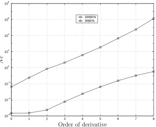
points as defined in (21). Results ofN eobtained by two approaches using the same

network parameters (β = 1, n = m = 21, n_t = 101) are displayed in Figure 1,

which show that the performance of the indirect approach is clearly superior to

that of the direct approach on both function and derivative approximations. For

both approaches, the error norm is an increasing function of the order of derivative.

Some plots of derivatives are displayed in Figure 2, which indicates that the direct

while the indirect approach is able to capture all the derivative functions. For low

orders, there is no discernible difference between the IRBF and the exact solutions

(Figure 2).

In the case of the indirect approach, two aspects are further studied here. Firstly,

how does the “order” of the IRBFN scheme affect the accuracy of numerical solution.

Theith order IRBFN scheme, IRBFN-i, is regarded as an indirect scheme in which

the ith order derivative is decomposed into a set of RBFs. There are two concepts

of the order used throughout the present study, namely the order of derivative/ODE

and the order of an IRBFN scheme. To represent anith order derivative, the indirect

scheme needs be employed with at least ith order. Increasing the order of IRBFN

can improve the solution accuracy as shown in Figure 3. Secondly, the effect of β

on the solution accuracy is also investigated. It is known that large or small values

of the RBF width make the response of the corresponding basis function too flat or

too peaked respectively and therefore both of these two extreme conditions should

be avoided (Haykin [29]). Figure 4 shows that better approximations are obtained

with an increase in β up to the value of about 7.

The approximation of 6th order derivative of function (23) is reconsidered. By

increasing

• the value ofβ up to 7, or

• the order of IRBFN up to 10, or

• a number of centres up to 41,

the obtained solution is improved as displayed in Figure 5. The corresponding

error-nomrs are reduced from 0.0245 (IRBFN-8, β = 1) to 0.0030 (IRBFN-8, β = 7),

5.2

High order ODEs

The theoretical determinant for the optimum value of the RBF width has not been

established yet. For the approximation of a function and its derivatives, the

numer-ical example above indicated that the indirect approach performs well for a wide

range ofβ. In solving second order DEs (Mai-Duy and Tran-Cong [16]), experience

showed that the value of β can be chosen in the range 1 ≤ β ≤10. In the present

study, all values ofβ are simply fixed to be 7. Furthermore, the order of IRBFN is

chosen to be the same as that of ODE. In the indirect approach, Gaussian elimination

is applied to solve the systems of equations because all design matrices obtained here

are square. In the direct approach, the design matrices are non-square so that the

corresponding systems are solved in the least square sense unless otherwise stated.

5.2.1 Fourth order ODE - Boundary value problem

The problem here is to find a function y(x) satisfying the following fourth order

ODE

x4y[4]−4x3y+x2(12−x2)y+ 2x(x2−12)y+ 2(12−x2)y= 2x5, (24)

over a specified interval of thexaxis, 1≤x≤11, subject to the boundary conditions

fory and y at both ends of the domain. Note that this is a nonhomogeneous ODE

with coefficients being functions of x. The exact solution of (24) can be verified to

be

y=x+x2−x3+xexp(x) +xexp(−x).

To study convergence, four sets of 6, 11, 17 and 21 equally spaced points (m =n =

{6,11,17,21}) are employed for the design of networks in both DRBF and IRBF

transformed into

x4 m

i=1

w(i)h(_[4]i)(x)−4x3 m

i=1

w(i)h(_[3]i)(x) +x2(12−x2) m

i=1

w(i)h(_[2]i)(x)

+ 2x(x2−12) m

i=1

w(i)h(_[1]i)(x) + 2(12−x2) m

i=1

w(i)g(i)(x) = 2x5, (25)

m

i=1

w(i)g(i)(1) = 1 + exp(1) + exp(−1), (26)

m

i=1

w(i)h(_[1]i)(1) = 2 exp(1), (27)

m

i=1

w(i)g(i)(11) = 11 + 112−113+ 11 exp(11) + 11 exp(−11), (28)

m

i=1

w(i)h(_[1]i)(11) = 1 + 2(11)−3(11)2+ 12 exp(11)−10 exp(−11), (29)

for the direct approach and

x4 m

i=1

w(i)g(i)(x)−4x3 m+1

i=1

w(i)H_[3](i)(x) +x2(12−x2) m+2

i=1

w(i)H_[2](i)(x)

+ 2x(x2−12) m+3

i=1

w(i)H_[1](i)(x) + 2(12−x2) m+4

i=1

w(i)H_[0](i)(x) = 2x5, (30)

m+4 i=1

w(i)H_[0](i)(1) = 1 + exp(1) + exp(−1), (31)

m+3 i=1

w(i)H_[1](i)(1) = 2 exp(1), (32)

m+4 i=1

w(i)H_[0](i)(11) = 11 + 112−113+ 11 exp(11) + 11 exp(−11), (33)

m+3 i=1

w(i)H_[1](i)(11) = 1 + 2(11)−3(11)2+ 12 exp(11)−10 exp(−11), (34)

for the indirect approach, in which the unknowns are network weights {w(i)}_{. The}

evaluation of (25) or (30) at a set of collocation points{x(i)}n_i=1plus the discretization

the form

Aw =b,

where A is an (n+ 4)−by−m matrix for the direct approach and an (n+ 4)−

by−(m + 4) matrix for the indirect approach. For all study cases, error norms

of the solution y are calculated at a test set of 101 uniformly distributed points.

Figure 6 shows that the indirect approach yields very accurate results and also a

high convergence rate while the opposite is true for the direct approach. Solutions

converge apparently as O(h−0.0447) and O(h7.1594) with h being the centre spacing

for the direct and indirect approaches respectively. At the finest discretization used

here (i.e. 21 training data points), error norms of the solution are 2.48 and 1.23e−6

for the direct and indirect approaches respectively.

It can be seen from Figure 6 that the performance of the direct approach is very

poor, for example, no “mesh” convergence is observed there. As discussed above,

the obtained system is overdetermined for the direct approach, but determined for

the indirect approach. The question here is whether the performance of the direct

approach can be improved when its design matrices are square. To make the matrix

of the direct approach square, the following relation needs be satisfied

n+p=m, (35)

where p is the order of ODE. In other words, the number of collocation points

used to approximate the strong form of the governing equation must be chosen less

than the number of centres (i.e. n < m). For the problem under consideration

here, by not applying the ODE at two boundary points together with two interior

points (for example, interior points adjacent to the boundaries are set aside here),

the relation (35) is satisfied and Gaussian elimination can be applied to solve the

where the convergence rate is of O(h2.1744_{) (h is the centre spacing) and the error}

norm is 0.0591 at the finest discretization. However, they are still far less accurate

than those obtained by the proposed indirect approach and also have much lower

convergence rate.

5.2.2 Fourth order ODE - Eigenvalue problem

Consider the transverse vibration of an uniform beam of length l for which the

general equation takes the form

∂4y ∂x4 +

ρA EI

∂2y

∂t2 = 0, (36)

where ρ, E and I are the mass per unit length, the elastic module and the area

moment of inertia about the neutral axis respectively. Assuming that the deflection

at any point of the beam varies harmonically with time

y(x, t) =φ(x)sin(ωt). (37)

Substitution of (37) into (36) yields

∂4φ ∂x4 −λ

4_{φ= 0, (38)}

where λ4 = ρAω2/EI. The following are three types of boundary condition to be

considered here

• Pinned-pinned beam

• Clamped-clamped beam

φ(0) =φ(0) = 0, φ(l) = φ(l) = 0; (40)

• Clamped-pinned beam

φ(0) =φ(0) = 0, φ(l) =φ(l) = 0. (41)

Eigenvalue problems require more effort to form the final system of equations than

boundary value problems. Substitution of the closed form IRBFN representations

of the variable φ and its derivatives (6)-(10) into the governing equation (38) and

also boundary conditions, e.g. (39) for the case of pinned-pinned beam, yields

m

i=1

w(i)g(i)(x)−λ4 m+4

i=1

w(i)H_[0](i)(x) = 0, (42)

m+4 i=1

w(i)H_[0](i)(0) = 0, (43)

m+2 i=1

w(i)H_[2](i)(0) = 0, (44)

m+4 i=1

w(i)H_[0](i)(l) = 0, (45)

m+2 i=1

w(i)H_[2](i)(l) = 0, (46)

or in the matrix form,

Aw−λ4Bw = 0, (47)

or

(A₁,A₂)(w₁,w₂)T −λ4(B₁,B₂)(w₁,w₂)T = 0, (49)

(C₁,C₂)(w₁,w₂)T = 0, (50)

where the dimensions of submatrices aren×n(A₁),n×p(A₂),n×n(B₁),n×p(B₂),

p×n(C₁), p×p(C₂), 1×n(w₁) and 1×p(w₂) in which n and pare the number of

collocation points (centres) and the order of ODE respectively (p= 4 here). With

some manipulations on (49) and (50), the final system of equations takes the form

[(A₁−A₂C₂−1C₁)−λ4(B₁ −B₂C−₂1C₁)]w₁T =0. (51)

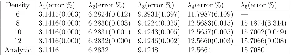
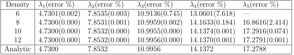
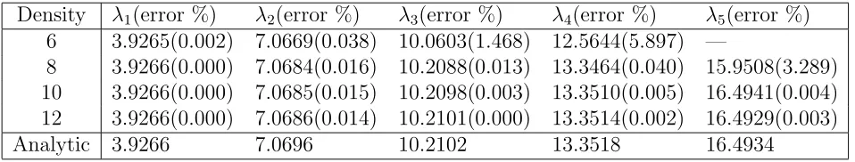
Results ofλobtained withl = 1 are displayed in Tables 1, 2 and 3 for pinned-pinned,

clamped-clamped and clamped-pinned beams respectively. The analytic solution is

also given for comparison. The proposed method achieves accurate results and also

high rates of convergence for all study cases.

It is observed that when increasing data densities, the computed results are

consis-tently more accurate, but their values slightly oscillate about the exact values, e.g.

the case: λ₄, pinned-pinned beam (Table 1). The reason for this behaviour is not

clear, probably due to the combined effect of the centre density and the value of β.

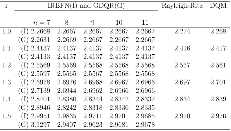
5.2.3 Sixth order ODE - Vibrations of ring-like structures

The vibrational behaviour of ring-like structures, which is important in engineering

applications, is considered in this section. The vibration problem governed by the

sixth order differential equation was studied by Gutierrez and Laura [6] using the

differential quadrature method (DQM) and the optimized Rayleigh-Ritz method

The structural element is a ring of rectangular cross-section of constant width and

thickness which varies parabolically according to the relation (Figure 7):

h( ¯α) =h(0)

− 4

π2(r−1) ¯α

2₊ 4

π(r−1) ¯α+ 1

=h(0)f( ¯α), (52)

wherer =h(π/2)/h(0). The case of normal, in-plane modes of vibration is studied

here, where only flexural effects are taken into account and one disregards stretching

in the axial direction.

A circular ring with supports (Figure 7-a): Since the structure is symmetric,

only half of the domain is considered. Introducing the dimensionless variable α =

¯

α/π, the governing differential equation can be expressed in the form

β₁v[6]+β₂v[5]+β₃v[4]+β₄v +β₅v +β₆v −Ω2

f v+fv −π2f v

= 0, (53)

subject to the boundary conditions

v(0) =v(0) =v(0) = 0, v(1) =v(1) =v(1) = 0,

wherev is the tangential displacement, Ω is the dimensionless frequency and

0 ≤ α≤1

β₁ = φ/π4, β₂ = 3φ/π4, β₃ = (2φ/π2) + (3φ/π4),

β₄ = (4φ/π2) + (φ/π4), β₅ =φ+ (3φ/π2), β₆ =φ+ (φ/π2), φ = [f(α)]3.

The solution procedures are similar to the problem of transverse vibration of a beam

in the previous section and therefore omitted here for brevity. Five data sets of 6, 7,

coefficients of in-plane, inextensional vibration obtained are listed in Table 4. The

values predicted by the DQM, the optimized Rayleigh-Ritz method and the GDQR

method are also given for comparison purpose. Good agreements are observed.

Both GDQR and IRBF collocation methods yield good results even if only 8 points

are used for r < 1.4. For the DQM, it was found necessary to take n = 12 for

r={1.0; 1.1; 1.2; 1.3} and n= 14 for r ={1.4; 1.5} (Gutierrez and Laura [6]).

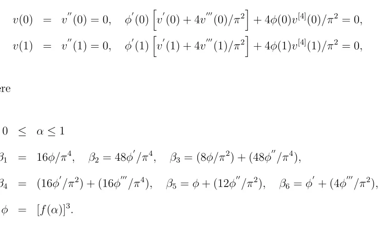
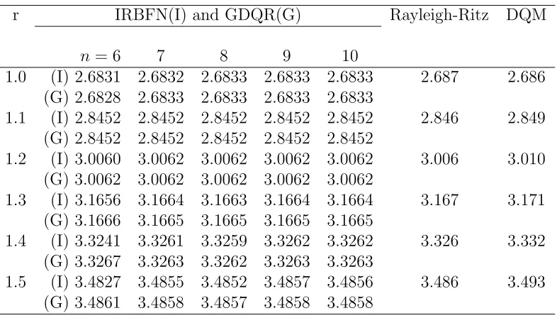
A completely free ring(Figure 7-b): In this case, a quarter of the ring structure

is considered. It is convenient to introduce the dimensionless variable α = 2 ¯α/π

here and the governing equations can be written as

β₁v[6]+β₂v[5]+β₃v[4]+β₄v+β₅v+β₆v−Ω2

f v +fv−π2f v/4

= 0, (54)

subject to the boundary conditions

v(0) = v(0) = 0, φ(0)

v(0) + 4v(0)/π2

+ 4φ(0)v[4](0)/π2 = 0,

v(1) = v(1) = 0, φ(1)

v(1) + 4v(1)/π2

+ 4φ(1)v[4](1)/π2 = 0,

where

0 ≤ α≤1

β₁ = 16φ/π4, β₂ = 48φ/π4, β₃ = (8φ/π2) + (48φ/π4),

β₄ = (16φ/π2) + (16φ/π4), β₅ =φ+ (12φ/π2), β₆ =φ+ (4φ/π2), φ = [f(α)]3.

Table 5 displays the results obtained by the present method together with those

obtained by the DQM, GDQR and Rayleigh-Ritz methods. Values differ only in

the third or fourth significant digit so all solutions are reasonable approximations.

IRBF collocation methods. Note that the DQM was reported to use 12 data points

for this case.

5.2.4 Eighth order ODE - Initial value problem and boundary value

problem

The unsymmetric IRBF collocation method is further verified here in the solution

of eighth order ODE

y[8]+y[7]+y[6]+y[5]+y[4]+y+y+y+y= 9 exp(x), (55)

over the interval 0≤x≤1.

Firstly, the initial value problem governed by (55) with initial values

y(0) =y(0) =y(0) =y(0) =y[4](0) =y[5](0) =y[6](0) =y[7](0) = 1, (56)

is considered. The exact solution of (55) and (56) can be verified to bey(x) = exp(x).

A number of uniform data sets whose sizes vary from 3 to 6 with an increment of 1

are chosen to be the sets of centres. For comparison purpose, the fourth order

Runge-Kutta method is also applied here to solve this problem using the same data sets, in

which the centre spacing is interpreted as time step. Good accuracy and high rate

of convergence are obtained for both methods especially for the proposed method

(Figure 8). Solutions converge apparently asO(h3.8408) and O(h5.8484) with h being

the centre spacing for the Runge-Kutta and IRBF collocation methods respectively.

The present method achieves error-norms at least three order lower than the

Runge-Kutta method. For example, at the centre spacing of 1/5, error-norms are 8.70e−6

Secondly, the boundary value problem governed by the eighth order ODE above is

considered. Four boundary conditions fory, y, yandy[3]whose values are computed

from the exact solutiony(x) = exp(x) are imposed at both-ends of the domain. Five

data densities of 5, 6, 7, 8 and 9 equally spaced points together with 101 test points

are employed to investigate this problem. The proposed method yields very good

results for all densities with the corresponding error-norms being 4.48e−13,9.34e−

14,1.54e−14,4.70e−15 and 1.32e−15 respectively. Figure 9 shows that a high

convergence rate up to O(h8.4703_{) (h is the centre spacing) is achieved with the}

present method.

5.2.5 Eighth order ODE - Simply supported single-barrel shell with free

edges

This problem is taken from reference (Kelkar and Sewell [33]) and was studied by Wu

and Liu [9] using the GDQR (Figure 10). The shell parameters are a longitudinal

length of L = 42 ft, a barrel radius of a = 12.5 ft and a shell thickness of t = 0.25

ft. The half angle of the barrel is 40o. The circular cylindrical single-barrel roof is

free at the two edges along the longitudinal x-direction with 0≤x≤L and simply

supported at the other two circular edges x = 0 and x = L. An equivalent dead

distributed load of p= 62.5 lb/ft2 is considered. Since the L/aratio is greater than

3, the Schorer theory can be applied to solve this problem. The shell only for the

first harmonic of the Fourier series expansion for the loading is analyzed here. The

radial displacement is thus expressed as follows

v(x, φ) =V(φ) sinπx

The analysis of Kelkar and Sewell [33] leads to the following governing eighth order

ODE

V[8]+λ8V =−−8pa

4_cosφ

πK , (58)

subject to the four boundary conditions for stress at free edges as follows

M_φ = 0, Q_φ = 0, N_φ= 0 and N_xφ= 0, (59)

whereλ8 = 12π4a6/(L4t2),K =Et3/12 andE is the Young’s modulus.

The solution V can be decomposed into a homogeneous part Vh and a particular

solution partVp as

V =Vh+Vp.

The membrane solution is adopted as the particular solution whose form for some

bending stresses of particular interest here is

M_φp = 0, (60)

Qp_φ = 0, (61)

N_φp = −4pa

π cosφsin

πx

L , (62)

N_xφp = 8pL

π2 sinφcos πx

L , (63)

N_xp = −8pL

2

π3a cosφsin πx

L . (64)

resultants are given by

M_φh = K

a2 d2V

dφ2 sin πx

L , (65)

Qh_φ = K

a3 d3V

dφ3 sin πx

L , (66)

N_φh = −K

a3 d4V

dφ4 sin πx

L , (67)

N_xφh = −KL

πa4 d5V

dφ5 cos πx

L , (68)

N_xh = KL

2

π2a5 d6V

dφ6 sin πx

L , (69)

The task now is to find the solution of the homogeneous governing equation

corre-sponding to (58)

Vh[8]+λ8Vh = 0, (70)

subject to the four boundary conditions at each edge

M_φh =−M_φp, Qh_φ=−Qp_φ, N_φh =−N_φp and N_xφh =−N_xφp ,

or

d2Vh dφ2 = 0,

d3Vh dφ3 = 0,

d4Vh

dφ4 =−

4pa4

πK cosφ, and

d5Vh

dφ5 =

8pa4

πK sinφ. (71)

The unsymmetric IRBF collocation procedure to solve (70)-(71) is similar to the

previous numerical examples. Results obtained (Vh _{and its derivatives) are then}

substituted into (65)-(69) to produce the force and moment resultants. The analytic

homogeneous results can be found in (Kelkar and Sewell [33]) and (Wu and Liu [9]).

Note that the coefficients of the analytic results provided in (Kelkar and Sewell [33])

are only accurate to two significant figures. To obtain higher accuracy, Wu and Liu

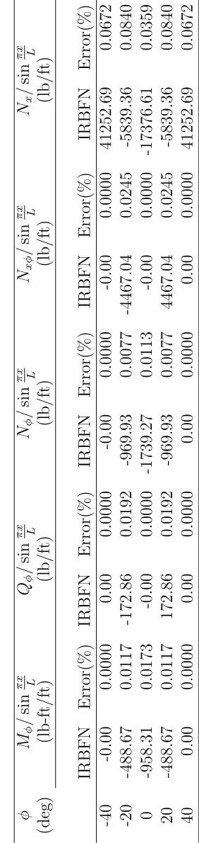
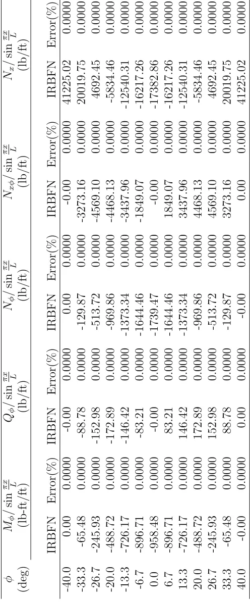
used here for comparison. Tables 6-8 present the final computed force and moment

resultants using 5, 9 and 13 equally spaced points. With only a few equally spaced

points, the IRBF results are in very good agreement with the analytic results. It also

shows that the finer density yields a better approximation to the true value. The

difference is less than 0.085 % in all cases. At the finest data density (n = 13), the

maximum error is 0.00004%. It is remarkable because the computed stress resultants

here involve derivatives up to 7th order. For the GDQR method, the cosine-type of

the sampling points is employed. With the same numbers of data points used (i.e.

5, 9 and 13 points), the maximum error of the force and moment resultants is about

0.62% (Wu and Liu [9]), which is slightly greater than that obtained by the present

method (0.085%).

6

CONCLUDING REMARKS

This paper reports new meshless numerical methods based on RBFNs for solving

high order ODEs directly. Two unsymmetric RBF collocation approaches are

em-ployed to approximate the strong form of the governing equations and the boundary

conditions. Like other meshless numerical methods (e.g. smoothed particle

hydro-dynamics, the vortex method, the generalized finite difference method and many

others), the direct RBF collocation approach here is based on the differential

pro-cess to represent the solution. By contrast, in the proposed indirect RBF collocation

approach, the closed forms representing the dependent variable and its derivatives

are obtained through the integration process. The use of the integration process

results in higher approximation power for RBFNs. Furthermore, in the case of

solv-ing high order ODEs, the well-known difficulties to deal with multiple boundary

conditions are naturally overcome via means of integration constants. Two present

and initial value problems. It requires no extra effort when increasing the order

of ODE. Analytic and numerical techniques for obtaining new basis functions from

RBFs are discussed. Among RBFs, multiquadrics are preferred for practical use.

Numerical results show that the proposed indirect approach performs much better

than the usual direct approach. High convergence rates and good accuracy are

ob-tained with the proposed method using relatively low numbers of data points. The

proposed unsymmetric IRBF collocation method can be extended to the solution of

APPENDIX

The following are new basis functions derived from RBFs by using

MATHEMAT-ICA.

Direct approach - Multiquadrics

h(_[1]i) = x−c(i) [(x−c(i))2+a(i)2]1/2, h(_[2]i) = a(i)2

[(x−c(i))2+a(i)2]3/2, h(_[3]i) = −3a(i)2(x−c(i))

[(x−c(i))2+a(i)2]5/2, h(_[4]i) = 3a(i)2[4(x−c(i))2−a(i)2]

[(x−c(i))2+a(i)2]7/2 ,

h(_[5]i) = −15a(i)2(x−c(i))[4(x−c(i))2−3a(i)2] [(x−c(i))2+a(i)2]9/2 , h(_[6]i) = 45a(i)2[8(x−c(i))4−12a(i)2(x−c(i))2+a(i)4]

[(x−c(i))2+a(i)2]11/2

h(_[7]i) = −315a(i)2(x−c(i))[8(x−c(i))4−20a(i)2(x−c(i))2+5a(i)4] [(x−c(i))2+a(i)2]13/2 ,

h(_[8]i) = 315a(i)2[64(x−c(i))6−240a(i)2(x−c(i))4+120a(i)4(x−c(i))2−5a(i)6] [(x−c(i))2+a(i)2]15/2 .

Direct approach - Gaussians

h(_[1]i) = −2(x−c(i)) a(i)2 exp

−(x−c(i))2 a(i)2

,

h(_[2]i) = 2[2(x−c(i))2−a(i)2]

a(i)4 exp

−(x−c(i))2 a(i)2

,

h(_[3]i) = −4(x−c(i))[2(x−c(i))2−3a(i)2]

a(i)6 exp

−(x−c(i))2 a(i)2

,

h(_[4]i) = 4[4(x−c(i))4−12(x−c(i))2a(i)2+3a(i)4]

a(i)8 exp

−(x−c(i))2 a(i)2

,

h(_[5]i) = −8(x−c(i))[4(x−c(i))4−20(x−c(i))2a(i)2+15a(i)4]

a(i)10 exp

−(x−c(i))2 a(i)2

,

h(_[6]i) = 8[8(x−c(i))6−60(x−c(i))4a(i)2+90(x−c(i))2a(i)4−15a(i)6]

a(i)12 exp

−(x−c(i))2 a(i)2

,

h(_[7]i) = −16(x−c(i))[8(x−c(i))6−84(x−c(i))4a(i)2+210(x−c(i))2a(i)4−105a(i)6]

a(i)14 exp

−(x−c(i))2 a(i)2

,

h(_[8]i) = 16[16(x−c(i))8−224(x−c(i))6a(i)2+840(x−c(i))4a(i)4−840(x−c(i))2a(i)6+105a(i)8]

a(i)16 exp

−(x−c(i))2 a(i)2

Indirect approach - Multiquadrics

H_[1](i) = (x−₂c(i))A+ a(₂i)2B,

H_[2](i) =

−a(i)2

3 + (x−c

(i)₎2

6

A+ a(i)2(x₂−c(i))B,

H_[3](i) =

−13a(i)2(x−c(i))

48 +(x−c

(i)₎3

24

A+

−a(i)4

16 + a

(i)2_(x−c(i)₎2

4

B,

H_[4](i) =

a(i)4

45 − 83a

(i)2_(x−c(i)₎2

720 + (x−c

(i)₎4

120

A+

−3a(i)4(x−c(i))

48 +4a

(i)2_(x−c(i)₎3

48

B,

H_[5](i) =

113a(i)4(x−c(i))

5760 − 97a

(i)2_(x−c(i)₎3

2880 +(x−c

(i)₎5

720

A+

a(i)6

384 −3a

(i)4_(x−c(i)₎2

96 + 2a

(i)2_(x−c(i)₎4

96

B,

H_[6](i) =

−a(i)6

1575 + 593a

(i)4_(x−c(i)₎2

67200 − 253a

(i)2_(x−c(i)₎4

33600 + (x−c

(i)₎6

5040

A

+

5a(i)6(x−c(i))

1920 −20a

(i)4_(x−c(i)₎3

1920 + 8a

(i)2_(x−c(i)₎5

1920

B,

H_[7](i) =

−1873a(i)6(x−c(i))

3225600 + 4327a

(i)4_(x−c(i)₎3

1612800 −551a

(i)2_(x−c(i)₎5

403200 +(x−c

(i)₎7

403200

A

+

−a(i)8

18432 + 15a

(i)6_(x−c(i)₎2

11520 − 30a

(i)4_(x−c(i)₎4

11520 +8a

(i)2_(x−c(i)₎6

11520

B,

H_[8](i) =

a(i)8

99225 −54511a

(i)6_(x−c(i)₎2

203212800 + 20939a

(i)4_(x−c(i)₎4

33868800 − 5309a

(i)2_(x−c(i)₎6

25401600 +(x−c

(i)₎8

362880

A

+

−35a(i)8(x−c(i))

645120 +280a

(i)6_(x−c(i)₎3

645120 −336a

(i)4_(x−c(i)₎5

645120 +64a

(i)2_(x−c(i)₎7

645120

B,

whereA=(x−c(i)₎2_+a(i)2 _{and B = ln(x}−_c(i)_{) +(x−c}(i)₎2_+a(i)2_.

ACKNOWLEDGEMENTS

The author is grateful to Professor R.I. Tanner for fruitful discussions and for

care-fully reading the paper and correcting errors. The author would like to thank the

referees for their helpful comments.

REFERENCES

1. Dahlquist G, Bjorck A, Anderson N. Numerical Methods; Prentice-Hall: New

Jersey, 1974.

2. Press WH, Flannery BP, Teukolsky SA, Vetterling WT.Numerical Recipes in

C: The Art of Scientific Computing; Cambridge University Press: Cambridge,

3. Viecelli JA. Exponential difference operator approximation for the sixth order

Onsager equation. Journal of Computational Physics 1983; 50: 162-170.

4. Sallam S, El-Hawary HM. A deficient spline function approximation of

second-order differential equations. Applied Mathematical Modelling 1984; 8(6):

408-412.

5. Esmail MN, Fawzy T, Ahmed M, Elmoselhi HO. A deficient spline function

approximation to fourth-order differential equations. Applied Mathematical

Modelling1994; 18(12): 658-664.

6. Gutierrez RH, Laura PAA. Vibrations of non-uniform rings studied by means

of the differential quadrature method. Journal of Sound and Vibration 1995;

185(3): 507-513.

7. Wu TY, Liu GR. Application of the generalized differential quadrature rule to

sixth-order differential equations. Communications in Numerical Methods in

Engineering2000; 16: 777-784.

8. Wu TY, Liu GR. The generalized differential quadrature rule for fourth-order

differential equations. International Journal for Numerical Methods in

Engi-neering2001; 50: 1907-1929.

9. Wu TY, Liu GR. Application of the generalized differential quadrature rule to

eighth-order differential equations. Communications in Numerical Methods in

Engineering2001; 17: 355-364.

10. Bellman R, Casti J. Differential quadrature and long term integration. Journal

of Mathematical Analysis and Application1971; 34: 235-238.

11. Wood HG, Morton JB. Onsager’s pancake approximation for the fluid

12. Kansa EJ. Multiquadrics-A scattered data approximation scheme with

appli-cations to computational fluid-dynamics-II. Solutions to parabolic, hyperbolic

and elliptic partial differential equations. Computers and Mathematics with

Applications1990; 19(8/9); 147-161.

13. Sharan M, Kansa EJ, Gupta S. Application of the multiquadric method for

numerical solution of elliptic partial differential equations. Journal of Applied

Science and Computation1997; 84: 275-302.

14. Zerroukat M, Power H, Chen CS. A numerical method for heat transfer

prob-lems using collocation and radial basis functions. International Journal for

Numerical Methods in Engineering 1998;42: 1263-1278.

15. Mai-Duy N, Tran-Cong T. Numerical solution of differential equations using

multiquadric radial basis function networks. Neural Networks 2001; 14(2):

185-199.

16. Mai-Duy N, Tran-Cong T. Numerical solution of Navier-Stokes equations

us-ing multiquadric radial basis function networks. International Journal for

Numerical Methods in Fluids2001; 37: 65-86.

17. Fedoseyev AI, Friedman MJ, Kansa EJ. Improved multiquadric method for

elliptic partial differential equations via PDE collocation on the boundary.

Computers & Mathematics with Applications2002; 43(3-5): 439-455.

18. Mai-Duy N, Tran-Cong T. Approximation of function and its derivatives using

radial basis function network methods. Applied Mathematical Modelling2003;

27: 197-220.

19. Jin X, Li G, Aluru NR. On the equivalence between least-squares and kernel

approximations in meshless methods. Computer Modeling in Engineering and

20. Atluri SN, Shen S. The Meshless Local Petrov-Galerkin Method; Tech Science

Press: Encino, 2002.

21. Li S, Liu WK. Meshfree and particle methods and their applications. Applied

Mechanics Reviews2002; 55(1): 1-34.

22. Liu GR. Mesh Free Methods - Moving Beyond The Finite Element Method;

CRC Press: Boca Raton, 2003.

23. Liu GR, Gu YT. A local radial point interpolation method (LRPIM) for free

vibration analyses of 2-D solids. Journal of Sound and Vibration2001;246(1):

29-46.

24. Wang JG, Liu GR. A point interpolation meshless method based on radial

basis functions. International Journal for Numerical Methods in Engineering

2002;54: 1623-1648.

25. Wang JG, Liu GR. On the optimal shape parameters of radial basis functions

used for 2-D meshless methods. Computer Methods in Applied Mechanics and

Engineering2002; 191: 2611-2630.

26. Wang JG, Liu GR, Lin P. Numerical analysis of Biot’s consolidation process

by radial point interpolation method. International Journal of Solids and

Structures 2002; 39(6): 1557-1573.

27. Gu YT, Liu GR. A boundary radial point interpolation method (BRPIM) for

2-D structural analyses. Structural Engineering and Mechanics 2003; 15(5):

535-550.

28. Wu YL, Liu GR. A meshfree formulation of local radial point interpolation

method (LRPIM) for incompressible flow simulation. Computational

29. Haykin S.Neural Networks: A Comprehensive Foundation; Prentice-Hall: New

Jersey, 1999.

30. Abramowitz M, Stegun IA. Handbook of Mathematical Functions; Dover

Pub-lications: New York, 1972.

31. Madych WR, Nelson SA. Multivariate interpolation and conditionally positive

definite functions. Approximation Theory and its Applications1989; 4: 77-89.

32. Madych WR, Nelson SA. Multivariate interpolation and conditionally positive

definite functions, II.Mathematics of Computation 1990;54(189): 211-230.

33. Kelkar VS, Sewell RT.Fundamentals of the Analysis and Design of Shell

Table 1: Fourth order ODE, free vibration, pinned-pinned beam: eigenvalues. For

each eigenvalue λ_i, the error is consistently reduced with increasing density.

Density λ₁(error %) λ₂(error %) λ₃(error %) λ₄(error %) λ₅(error %)

6 3.1415(0.003) 6.2824(0.012) 9.2931(1.397) 11.7987(6.109) —

8 3.1416(0.000) 6.2830(0.003) 9.4224(0.025) 12.5683(0.015) 15.1874(3.314)

10 3.1416(0.000) 6.2831(0.001) 9.4243(0.005) 12.5657(0.005) 15.7002(0.049)

12 3.1416(0.000) 6.2832(0.000) 9.4246(0.002) 12.5660(0.003) 15.7066(0.008)